The coefficient of determination R² and intra-class correlation coefficient from generalized linear mixed-effects models revisited and expanded

Abstract

The coefficient of determination R² quantifies the proportion of variance explained by a statistical model and is an important summary statistic of biological interest. However, estimating R² for generalized linear mixed models (GLMMs) remains challenging. We have previously introduced a version of R² that we called for Poisson and binomial GLMMs, but not for other distributional families. Similarly, we earlier discussed how to estimate intra-class correlation coefficients (ICCs) using Poisson and binomial GLMMs. In this paper, we generalize our methods to all other non-Gaussian distributions, in particular to negative binomial and gamma distributions that are commonly used for modelling biological data. While expanding our approach, we highlight two useful concepts for biologists, Jensen's inequality and the delta method, both of which help us in understanding the properties of GLMMs. Jensen's inequality has important implications for biologically meaningful interpretation of GLMMs, whereas the delta method allows a general derivation of variance associated with non-Gaussian distributions. We also discuss some special considerations for binomial GLMMs with binary or proportion data. We illustrate the implementation of our extension by worked examples from the field of ecology and evolution in the R environment. However, our method can be used across disciplines and regardless of statistical environments.

1. Introduction

One of the main purposes of linear modelling is to understand the sources of variation in biological data. In this context, it is not surprising that the coefficient of determination R² is a commonly reported statistic, because it represents the proportion of variance explained by a linear model. The intra-class correlation coefficient (ICC) is a related statistic that quantifies the proportion of variance explained by a grouping (random) factor in multilevel/hierarchical data. In the field of ecology and evolution, a type of ICC is often referred to as repeatability R, where the grouping factor is often individuals that have been phenotyped repeatedly [1,2]. We have reviewed methods for estimating R² and ICC in the past, with a particular focus on non-Gaussian response variables in the context of biological data [2,3]. These previous articles featured generalized linear mixed-effects models (GLMMs) as the most versatile engine for estimating R² and ICC (specifically and ICC_GLMM). The descriptions were initially limited to random-intercept GLMMs, but have later been extended to random-slope GLMMs [4], widening the applicability of these statistics (see also [5,6]).

However, at least one important issue seems to remain. Currently, these two statistics are only described for binomial and Poisson GLMMs. Although these two types of GLMM are arguably the most popular [7], there are other families of distributions that are commonly used in biology, such as negative binomial and gamma distributions [8,9]. In this paper, we revisit and extend and ICC_GLMM to more distributional families with a particular focus on negative binomial and gamma distributions. In this context, we discuss Jensen's inequality and two variants of the delta method, which are hardly known among biologists. These concepts are useful not only for generalizing our previous methods, but also for interpreting the results of GLMMs. Furthermore, we refer to some special considerations when obtaining and ICC_GLMM from binomial GLMMs for binary and proportion data, which we did not discuss in the past [2,3]. We provide worked examples inspired from the field of ecology and evolution, focusing on implementation in the R environment [10] and finish by referring to two alternative approaches for obtaining R² and ICC from GLMMs along with a cautionary note.

2. Definitions of , ICC_GLMM and overdispersion

To start with, we present and ICC_GLMM for a simple case of Gaussian error distributions based on a linear mixed-effects model (LMM, hence also referred to as and ICC_LMM). Imagine a two-level dataset where the first level corresponds to observations and the second level to some grouping/clustering factor (e.g. individuals with repeated measurements) with k fixed-effect covariates. The model can be written as (referred to as Model 1):

2.1

2.2

2.3

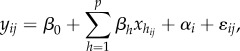
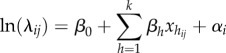
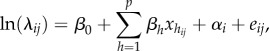
where y_ij is the jth observation of the ith individual, is the jth value of the ith individual for the hth of k fixed-effect predictors, β₀ is the (grand) intercept, β_h is the regression coefficient for the hth predictor, α_i is an individual-specific effect, assumed to be normally distributed in the population with the mean and variance of 0 and , ɛ_ij is an observation-specific residual, assumed to be normally distributed in the population with mean and variance of 0 and , respectively. For this model, we can define two types of R² as

2.4

2.5

2.6

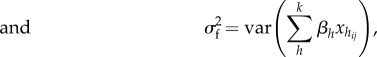
where represents the marginal R², which is the proportion of the total variance explained by the fixed effects, represents the conditional R², which is the proportion of the variance explained by both fixed and random effects, and is the variance explained by fixed effects [11]. As marginal and conditional R² differ only in whether the random effect variance is included in the numerator, we avoid redundancy and present equations only for marginal R² in the following.

Similarly, there are two types of ICC:

2.7

and

2.8

If no fixed effects are fitted (other than the intercept), so that ICC_LMM(adj) equals ICC_LMM. In such a case, the ICC should not be called ‘adjusted’ (sensu [2]). For an ICC value to be adjusted for a source of variance, that variance must be more than 0 and omitted from the ICC calculation. As the two versions of ICC differ only in whether the fixed-effect variance, calculated as in equation (2.6), is included in the denominator, we avoid redundancy and present equations only for adjusted ICC in the following.

One of the main difficulties in extending R² from LMMs to GLMMs is defining the residual variance . For binomial and Poisson GLMMs with an additive dispersion term, we have previously stated that is equivalent to where is the variance for the additive overdispersion term, and is the distribution-specific variance [2,3]. Here, overdispersion represents the excess variation relative to what is expected from a certain distribution and can be estimated by fitting an observation-level random effect (OLRE; [12,13]). Alternatively, overdispersion in GLMMs can be implemented using a multiplicative overdispersion term [14]. In such an implementation, we stated that is equivalent to where ω is a multiplicative dispersion parameter estimated from the model [2]. However, obtaining for specific distributions is not always possible, because in many families of GLMMs, (observation-level variance) cannot be clearly separated into (overdispersion variance) and (distribution-specific variance). It turns out that binomial and Poisson distributions are special cases where can be usefully calculated, because either all overdispersion is modelled by an OLRE (additive overdispersion) or by a single multiplicative overdispersion parameter (multiplicative overdispersion). This is not the case for other families. However, as we will show below, we can always obtain the GLMM version of (on the latent scale) directly. We refer to this generalized version of as ‘the observation-level variance’ here rather than the residual variance (but we keep the notation ). Note that the observation-level variance, , should not be confused with the variance associated with OLRE, which estimates and can be considered to be a part of .

3. Extension of and ICC_GLMM

We now define and ICC_GLMM for a quasi-Poisson (may also be referred to as overdispersed Poisson) GLMM, because the quasi-Poisson distribution is an extension of Poisson distribution [15,16] and is similar to the negative binomial distribution, at least in their common applications [9,17]. Imagine count data repeatedly measured from a number of individuals with associated data on k covariates. We fit a quasi-Poisson (QP) GLMM with the log-link function (Model 2):

3.1

3.2

3.3

where y_ij is the jth observation of the ith individual and y_ij follows a quasi-Poisson distribution with two parameters, λ_ij and ω [15,16], ln(λ_ij) is the latent value for the jth observation of the ith individual, ω is the overdispersion parameter (when the multiplicative dispersion parameter ω is 1, the model becomes a standard Poisson GLMM), α_i is an individual-specific effect, assumed to be normally distributed in the population with the mean and variance of 0 and , respectively (as in Model 1), and the other symbols are the same as above. Quasi-Poisson distributions have a mean of λ and a variance of λω (table 1). For such a model, we can define and (adjusted) ICC_GLMM as

3.4

and

3.5

where the subscript of R² and ICC denotes the distributional family, here QP-ln for quasi-Poisson distribution with log link, the term ln(1 + ω/λ) corresponds to the observation-level variance (table 1; for derivation, see the electronic supplementary material, appendix S1), ω is the overdispersion parameter, and λ is the mean value of λ_ij. We discuss how to obtain λ in §5.

Table 1.

The observation-level variance for the three distributional families: quasi-Poisson, negative binomial and gamma with the three different methods for deriving : the delta method, lognormal approximation and the trigamma function, . when x follows gamma distribution. In the R environment, the function, trigamma can be used to obtain ; also note that ν is known as a shape parameter while κ is as a rate parameter in gamma distribution.

family	distributional parameters	mean (E[y]) variance (var[y])	link function	delta method	lognormal approximation	trigamma function
quasi-Poisson (QP)			log
Poisson (when ω = 1)	λ > 0 ω > 0		square-root	0.25ω	—
negative binomial (NB)			log
	λ > 0 θ > 0		square-root		—
gamma			log
	λ > 0 ν > 0		inverse (reciprocal)		—
gamma (alternative parameterization)			log
	ν > 0 κ > 0		inverse (reciprocal)		—

The calculation is very similar for a negative binomial (NB) GLMM with the log link (Model 3):

3.6

3.7

3.8

where y_ij is the jth observation of the ith individual and y_ij follows a negative binomial distribution with two parameters, λ_ij and θ, where θ is the shape parameter of the negative binomial distribution (given by the software often as the dispersion parameter), and the other symbols are the same as above. The parameter θ is sometimes referred to as ‘size’. Negative binomial distributions have a mean of λ and a variance of λ + λ²/θ (table 1). and (adjusted) ICC_GLMM for this model can be calculated as

3.9

and

3.10

Finally, for a gamma GLMM with the log link (Model 4):

3.11

3.12

3.13

where y_ij is the jth observation of the ith individual and y_ij follows a gamma distribution with two parameters, λ_ij and ν, where ν is the shape parameter of the gamma distribution (sometimes statistical programmes report 1/ν instead of ν; also note that the gamma distribution can be parametrized in alternative ways, table 1). Gamma distributions have a mean of λ and a variance of λ²/ν (table 1). and (adjusted) ICC_GLMM can be calculated as

3.14

and

3.15

4. Obtaining the observation-level variance by the ‘first’ delta method

For overdispersed Poisson, negative binomial and gamma GLMMs with log link, the observation-level variance can be obtained via the variance of the lognormal distribution (electronic supplementary material, appendix S1). This is the approach that has led to the terms presented above. There are two more alternative methods to obtain the same target: the delta method and the trigamma function. The two alternatives have different advantages and we will therefore discuss them in some detail in the following.

The delta method for variance approximation uses a first-order Taylor series expansion, which is often employed to approximate the standard error (error variance) for transformations (or functions) of a variable x when the (error) variance of x itself is known (see [18]; for an accessible reference for biologists, [19]). The delta method for variance approximation can be written as

4.1

where x is a random variable (typically represented by observations), f represents a function (e.g. log or square-root), var denotes variance and d/dx is a (first) derivative with respect to variable x. Taking derivatives of any function can be easily done using the R environment (examples can be found in the electronic supplementary material, appendices). It is the delta method that Foulley et al. [20] used to derive the distribution-specific variance for Poisson GLMMs as 1/λ (see also [21]). Given that in the case of Poisson distributions and , it follows that (note that for Poisson distributions without overdispersion, is equal to because ).

One clear advantage of the delta method is its flexibility. We can easily obtain the observation-level variance for all kinds of distributions/link functions. For example, by using the delta method, it is straightforward to obtain for the Tweedie distribution, which has been used to model non-negative real numbers in ecology (e.g. [22,23]). For the Tweedie distribution, the variance on the observed scale has the relationship where μ is the mean on the observed scale and φ is the dispersion parameter, comparable to λ and ω in equation (3.1), and p is a positive constant called an index parameter. Therefore, when used with the log-link function, can be approximated by according to equation (4.1). The lognormal approximation is also possible (see the electronic supplementary material, appendix S1; table 1).

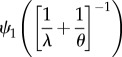
The use of the trigamma function is limited to distributions with log link, but it is considered to provide the most accurate estimate of the observation-level variance in those cases. This is because the variance of a gamma-distributed variable on the log scale is equal to where ν is the shape parameter of the gamma distribution [24] and hence is . At the level of the statistical parameters (table 1; on the ‘expected data’ scale; sensu [25]; see their fig. 1), both Poisson and negative binomial distributions can be seen as special cases of gamma distributions, and can be obtained using the trigamma function (table 1). For example, for the Poisson distribution is (note that ). 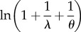As shown in the electronic supplementary material, appendix S2, ln(1 + 1/λ) (lognormal approximation), 1/λ (delta method approximation) and (trigamma function) give similar results when λ is greater than 2. Our recommendation is to use the trigamma function for obtaining whenever this is possible.

The trigamma function has been previously used to obtain observation-level variance in calculations of heritability (which can be seen as a type of ICC although in a strict sense, it is not; see [25]) using negative binomial GLMMs ([24,26]; cf. [25]). Table 1 summarizes observation-level variance for overdispersed Poisson, negative binomial and gamma distributions for commonly used link functions.

5. How to estimate λ from data

For some calculations, we require an estimate of the global expected value λ. Imagine a Poisson GLMM with log link and additive overdispersion fitted as an OLRE (Model 5):

5.1

5.2

5.3

5.4

where y_ij is the jth observation of the ith individual, and follows a Poisson distribution with the parameter λ_ij, e_ij is an additive overdispersion term for jth observation of the ith individual, and the other symbols are the same as above. Poisson distributions have a mean of λ and a variance of λ (cf. table 1). Using the lognormal approximation and (adjusted) ICC_GLMM can be calculated as

5.5

and

5.6

where, as mentioned above, the term ln(1 + 1/λ) is (or ) for Poisson distributions with the log link (table 1).

In our earlier papers, we proposed to use the exponential of the intercept, exp(β₀) (from the intercept-only model) as an estimator of λ [2,3]; note that exp(β₀) from models with any fixed effects will often be different from exp(β₀) from the intercept-only model. We also suggested that it is possible to use the mean of observed values y_ij. Unfortunately, these two recommendations are often inconsistent with each other. This is because, given Model 5 (and all the models in the previous section), the following relationships hold:

5.7

5.8

5.9

where E represents the expected value (i.e. mean) on the observed scale, β₀ is the mean value on the latent scale (i.e. β₀ from the intercept-only model), is the total variance on the latent scale (e.g. in Models 1 and 5, and in Models 2–4 [2]; see also [27]). In fact, exp(β₀) gives the median value of y_ij rather than the mean of y_ij, assuming a Poisson distribution. Thus, the use of exp(β₀) will often overestimate , providing smaller estimates of R² and ICC, compared to when using averaged y_ij (which is usually a better estimate of E[y_ij]). Quantitative differences between the two approaches may often be negligible, but when λ is small, the difference can be substantial so the choice of the method needs to be reported for reproducibility (electronic supplementary material, appendix S2). Our new recommendation is to obtain λ via equation (5.8), which is the Poisson parameter averaged across cluster-level parameters (λ_i for each individual in our example; [17,20,28]). Thus, obtaining λ via equation (5.8) will be more accurate than estimating λ by calculating the average of observed values although these two methods will give very similar or identical values when sampling is balanced (i.e. observations are equally distributed across individuals and covariates). This recommendation for obtaining λ also applies to negative binomial GLMMs (table 1).

6. Jensen's inequality and the ‘second’ delta method

A general form of equation (5.7) is known as Jensen's inequality, where g is a convex function. Hence, the transformation of the mean value is equal to or larger than the mean of transformed values (the opposite is true for a concave function; that is, ; [29]). In fact, whenever the function is not strictly linear, simple application of the inverse link function (or back-transformation) cannot be used to translate the mean on the latent scale into the mean value on the observed scale. This inequality has important implications for the interpretation of results from GLMMs, and also generalized linear models GLMs and linear models with transformed response variables.

Although log-link GLMMs (e.g. Model 5) have an analytical solution, equation (5.8), this is not usually the case. Therefore, converting the latent scale values into observation-scale values requires simulation using the inverse link function. However, the delta method for bias correction can be used as a general approximation to account for Jensen's inequality when using link functions or transformations. This application of the delta method uses a second-order Taylor series expansion [18,30]. A simple case of the delta method for bias correction can be written as

6.1

where d²/dx² is a second derivative with respect to the variable x and the other symbols are as in equations (4.1) and (5.8). By using this bias correction delta method (with ), we can approximate equation (5.8) using the same symbols as in equations (5.7)–(5.9):

6.2

The comparison between equation (5.8) (exact) and equation (6.2) (approximate) is shown in the electronic supplementary material, appendix S3. The approximation is most useful when the exact formula is not available as in the case of a binomial GLMM with logit link (Model 6):

6.3

6.4

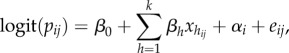
6.5

6.6

where y_ij is the number of ‘success’ in n_ij trials by the ith individual at the jth occasion (for binary data, n_ij is always 1), p_ij is the underlying probability of success, and the other symbols are the same as above. Binomial distributions have a mean of np and a variance of np(1 – p) (table 2).

Table 2.

The distribution-specific (theoretical) variance and observation-level variance using the delta method for binomial (and Bernoulli) distributions; note that only one of them should be used for obtaining R² and ICC. ‘erf⁻¹’ is the inverse of the Gauss error function, which is often denoted as ‘erf’.

family	distributional parameters, mean and variance	link name	link function	theoretical (distribution-specific) variance	observation-level variance (min. values and corresponding p given n = 1)
binomial (Bernoulli; n = 1)	binomial(n, p) 0 < p < 1 n ≥ 1 (integers)	logit		(logistic distribution)	(min = 4; p = 0.5)
	E[y] = np var[y] = np(1 – p) var[y/n] = p(1 – p)/n	probit ()		1(standard normal distribution)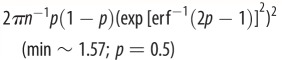
		cloglog (complimentary log–log)		(Gumbel distribution)	(min ∼ 1.54; p ∼ 0.8; ∼2.08; p = 0.5)

To obtain corresponding values between the latent scale and data (observation) scale, we need to account for Jensen's inequality. The logit function used in binomial GLMMs combines of concave and convex sections, which the delta method deals with efficiently. The overall intercept, β₀ on the latent scale could therefore be transformed not with the inverse (anti) logit function (), but with the bias-corrected delta method approximation. Given that in the case of the binomial GLMM with the logit-link function, the approximation can be written as (when n = 1)

6.7

We can replace β₀ with any value obtained from the fixed part of the model (i.e. ). McCulloch et al. [31] provide another approximation formula, which, by using our notation, can be written as

6.8

Yet, another approximation proposed by Zeger et al. [32] can be written as

6.9

This approximation, equation (6.9), uses the exact solution for the inverse probit function, which can be written for a model like Model 6 but using the probit link: i.e. probit 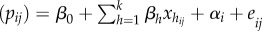in place of equation (6.4):

6.10

A comparison among equations (6.7)–(6.9) is also shown in electronic supplementary material, appendix S3 (it turns out equation (6.8) gives the best approximation). Simulation will give the most accurate conversions when no exact solutions are available. The use of the delta method for bias correction accounting for Jensen's inequality is a very general and versatile approach that is applicable for any distribution with any link function (see the electronic supplementary material, appendix S3) and can save computation time. We note that the accuracy of the delta method (both variance approximation and bias correction) depends on the form of the function f, the conditions for and limitation of the delta method are described by Oehlert [30].

7. Special considerations for binomial GLMMs

The observation-level variance can be thought of as being added to the latent scale on which other variance components are also estimated in a GLMM (equations (3.2), (3.7), (3.12), (5.2) and (6.4) for Models 2–6). As the proposed and ICC_GLMM are ratios between variance components and their sums, we can show using the delta method that and ICC_GLMM calculated via approximate to those of R² and ICC on the observation (original) scale (shown in the electronic supplementary material, appendix S4). In some cases, there exist specific formulae for ICC on the observation scale [2]. In the past, we distinguished between ICC on the latent scale and on the observation scale [2]. Such a distinction turns out to be strictly appropriate only for binomial distributions but not for Poisson distributions (and probably also not for other non-Gaussian distributions). This is because the property of what we have called the distribution-specific variance for binomial distributions (e.g. π²/3 for binomial error distribution with the logit-link function) is quite different from what we have discussed as the observation-level variance although these two types of variance are related conceptually (i.e. both represents variance due to non-Gaussian distributions with specific link functions). Let us explain this further.

A binomial distribution with a mean of p (the proportion of successes) has a variance of p(1 – p)/n (the variance for the number of successes is np(1 – p); table 2). We find that the observation-level variance is 1/(np(1 – p)) using the delta method on the logit-link function (table 2). This observation-level variance 1/(np(1 – p)), or 1/(p(1 – p)) for binary data, is clearly different from the distribution-specific variance π²/3. As with the observation-level variance for the log-Poisson model (which is 1/λ and changes with λ; note that we would have called 1/λ the distribution-specific variance; [2,3]), the observation-level variance of the binomial distribution changes as p changes (see electronic supplementary material, appendix S5), suggesting these two observation-level variances (1/λ and 1/(np(1 – p)) are analogous while the distribution-specific variance π²/3 is not. Further, the minimum value of 1/(p(1 – p)) is 4, which is larger than π²/3 ≈ 3.29, meaning that the use of 1/p(1 – p) in R² and ICC for binary data will always produce larger values than those using π²/3. Consequently, Browne et al. [14] showed that ICC values (or variance partition coefficients, VPCs) estimated using π²/3 were higher than corresponding ICC values on the observation (original) scale using logistic-binomial GLMMs (see also [33]). Note that they only considered binary data, i.e. 1/(np(1 – p)), where n = 1, because all proportion data can be rearranged as binary responses with a grouping/clustering factor.

Then, what is π²/3? Three common link functions in binomial GLMMs (logit, probit and complementary log–log) all have corresponding distributions on the latent scale: the logistic distribution, standard normal distribution and Gumbel distribution, respectively. Each of these distributions has a theoretical variance, namely, π²/3, 1 and π²/6, respectively, which we previous referred to as distribution-specific variances [2,3] (table 2). As far as we are aware, these theoretical variances only exist for binomial distributions. The meaning of 1/(np(1 – p)), which is the variance on the latent scale that approximates to the variance due to binomial distributions on the observation scale is distinct from the meaning of π²/3, which is the variance of the latent distribution (i.e. the logistic distribution with the scale parameter being 1). The use of the theoretical variance will almost always provide different values of and ICC_GLMM from those using the observation-level obtained via the delta method (see the electronic supplementary material, appendix S5). This is because the use of π²/3 implicitly assumes all datasets have the same observation-level variance regardless of mean proportion (p) given the same number of trials (n). Therefore, we need distinguishing these theoretical variances from the observation-level variance. R² and ICC values using the theoretical distribution-specific variance might be rightly called the latent (link) scale (sensu [2]) whereas, as mentioned above, R² and ICC values using the observation-level variance estimate the counterparts on the observation (original) scale (cf. [25]).

8. Worked examples: revisiting the beetles

In the following, we present a worked example by expanding the beetle dataset that was generated for previous work [3]. In brief, the dataset represents a hypothetical species of beetle that has the following life cycle: larvae hatch and grow in the soil until they pupate, and then adult beetles feed and mate on plants. Larvae are sampled from 12 different populations (‘Population’; figure 1). Within each population, larvae are collected at two different microhabitats (Habitat): dry and wet areas as determined by soil moisture. Larvae are exposed to two different dietary treatments (Treatment): nutrient rich and control. The species is sexually dimorphic and can be easily sexed at the pupa stage (Sex). Male beetles have two different colour morphs: one dark and the other reddish brown (‘Morph’, labelled as A and B in figure 1). Sexed pupae are housed in standard containers until they mature (Container). Each container holds eight same-sex animals from a single population, but with a mix of individuals from the two habitats (N_[container] = 120; N_[animal] = 960).

Figure 1.

A schematic of how hypothetical datasets are obtained (see the main text for details).

We have data on five phenotypes, two of them sex-limited: (i) the number of eggs laid by each female after random mating which we had generated previously using Poisson distributions (with additive dispersion) and we revisit here for analysis with quasi-Poisson models (i.e. multiplicative dispersion), (ii) the incidence of endo-parasitic infections that we generated as being negative binomial distributed, (iii) body length of adult beetles which we had generated previously using Gaussian distributions and that we revisit here for analysis with gamma distributions, (iv) time to visit five predefined sectors of an arena (used as a measure of exploratory tendencies) that we generated as being gamma distributed, and (v) the two male morphs, which was again generated with binomial distributions (for the details of parameter settings, table 3). We use this simulated dataset to estimate and ICC_GLMM.

Table 3.

Parameter settings of regression coefficients (b) and variance components (σ²) for five datasets: (1) fecundity, (2) endoparasite, (3) size, (4) exploration and (5) morph; all parameters are set on the latent scale apart from the size data (see below).

response	intercept (b)	sex (b)	treatment (b)	habitat (b)	population (ς2)	container (ς2)	overdispersion (ς2)
fecundity: the number of eggs per female	1.1	—	0.5	0.1	0.4	0.05	0.1
parasite: the number of endoparasites per individual	1.8	−2	−0.8	0.7	0.5	0.8	—
size: the body length of an individuala	15	−3	0.4	0.15	1.3	0.3	1.2
exploration: the time taken visiting five sectors for an individual	4	−1	2	−0.5	0.2	0.2	—
morph colour morph of a male	−0.8	—	0.8	0.5	1.2	0.2	—

^aData for the six sets of models were simulated on the normal (Gaussian) scale but analysed assuming a gamma error structure with the log link so that estimations of these parameters will be on the log scale; note the overdispersion variance for this data is the residual variance.

All data generation and analyses were conducted in R 3.3.1 [10]. We used functions to fit GLMMs from the three R packages: (i) the glmmadmb function from glmmADMB [34], (ii) the glmmPQL function from MASS [35], and (iii) the glmer and glmer.nb functions from lme4 [36]. In table 4, we only report results from glmmadmb because this is the only function that can fit models with all relevant distributional families. All scripts and results are provided as an electronic supplementary material, appendix S6. In addition, electronic supplementary material, appendix S6 includes an example of a model using the Tweedie distribution, which was fitted by the cpglmm function from the cplm package [23]. Notably, our approach for is kindly being implemented in the rsquared function in the R package piecewiseSEM [37]. Another important note is that we often find less congruence in GLMM results from the different packages than those of LMMs. For example, GLMM using the gamma error structure with the log-link function (Size and Exploration models), glmmadmb and glmmPQL produced very similar results, while glmer gave larger R² and ICC values than the former two functions (for more details, see electronic supplementary material, appendix S6; also see [38]). Thus, it is recommended to run GLMMs in more than one package to check robustness of the results although this may not always be possible.

Table 4.

Mixed-effects model analysis of a simulated dataset estimating variance components and regression slopes for nutrient manipulations on fecundity, endoparasite loads, body length, exploration levels and male morph types; N_[population] = 12, N_[container] = 120 and N_[animal] = 960 (N_[male] = N_[female] = 480). 95% CI (confidence intervals) were calculated by the confint function in lme4. The observation-level variance was obtained by using the trigamma function. In the Morph models, both the observation-level variance and (theoretical) distribution-specific variance were used; note that ones in brackets use the distribution-specific variance for R² and ICC. ICC_[Container] is not a typical ‘repeatability’ but the proportion of variance due to the container effect beyond the population variance.

	fecundity models (log-link) quasi-Poisson mixed models		parasite models (log-link) negative binomial mixed models		size models (log-link) gamma mixed models		exploration models (log-link) gamma mixed models		morph models (logit-link) binomial (binary) mixed models
model name	null model	full model	null model	full model	null model	full model	null model	full model	null model	full model
fixed effects	b [95% CI]	b [95% CI]	b [95% CI]	b [95% CI]	b [95% CI]	b [95% CI]	b [95% CI]	b [95% CI]	b [95% CI]	b [95% CI]
intercept	1.630 [1.379, 1.882]	1.261 [0.989, 1.532]	0.766 [0.330, 1.202]	1.752 [1.282, 2.223]	2.682 [2.616, 2.689]	2.737 [2.699, 2.775]	4.752 [4.555, 4.949]	4.056 [3.842, 4.269]	−0.108 [−0.718, 0.501]	−0.740 [−1.450, −0.030]
treatment (experiment)	—	0.491 [0.391, 0.591]	—	−0.768 [−0.870, −0.667]	—	0.033 [0.023, 0.044]	—	2.007 [1.965, 2.050]	—	0.840 [0.422, 1.258]
habitat (wet)	—	0.152 [0.055, 0.249]	—	0.700 [0.599, 0.801]	—	0.009 [−0.001, 0.019]	—	−0.560 [−0.603, −0.518]	—	0.414 [0.002, 0.826]
sex (male)	—	—	—	−2.198 [−2.511, −1.884]	—	−0.213 [−0.230, −0.196]	—	−1.105 [−1.256, −0.955]	—	—
random effects	σ2	σ2	σ2	σ2	σ2	σ2	σ2	σ2	σ2	σ2
population	0.178	0.187	0.375	0.541	0.0026	0.0039	0.071	0.104	1.002	1.111
container	0.042	0.059	1.976	0.613	0.0140	0.0014	0.364	0.163	0.136	0.186
observation-level (distribution-specific)	0.477	0.349	0.873	0.397	0.0069	0.0064	1.664	0.118	4.010 (3.290)	4.010 (3.290)
fixed factors	—	0.066	—	1.479	—	0.0116	—	1.393	—	0.220
(%)	—	9.96	—	48.50	—	49.54	—	78.34	—	3.98 (4.57)
(%)	—	46.95	—	86.33	—	72.52	—	93.34	—	27.46 (31.55)
ICC[Population] (%)	25.33	31.30	11.53	34.44	11.38	33.17	3.40	26.94	19.48 (22.64;)	20.95 (24.23)
ICC[Container] (%)	5.94	9.79	60.80	39.02	59.57	12.37	17.34	42.34	2.64 (3.07;)	3.50 (4.05)
AIC	2498.8	2412.3	4342.6	3920.5	3379.9	3139.5	11223.8	9004.3	605.5	589.6

In all the models, estimated regression coefficients and variance components are very much in agreement with what is expected from our parameter settings (compare table 3 with table 4; see also electronic supplementary material, appendix S6). When comparing the null and full models, which had ‘sex’ as a predictor, the magnitudes of the variance component for the container effect always decrease in the full models. This is because the variance due to sex is confounded with the container variance in the null model. As expected, (unadjusted) ICC values from the null models are usually smaller than adjusted ICC values from the full models because the observation-level variance (analogous to the residual variance) was smaller in the full models, implying that the denominator of, for example, equation (3.5) shrinks. However, the numerator also becomes smaller for ICC values for the container effect from the parasite, size and exploration models so that adjusted ICC values are not necessarily larger than unadjusted ICC values. Accordingly, adjusted ICC_[container] is smaller in the parasite and size models but not in the exploration model. The last thing to note is that for the morph models (binomial mixed models), both R² and ICC values are larger when using the distribution-specific variance rather than the observation-level variance, as discussed above (table 4; see also electronic supplementary material, appendix S4).

9. Alternatives and a cautionary note

Here we extend our simple methods for obtaining and ICC_GLMM for Poisson and binomial GLMMs to other types of GLMMs such as negative binomial and gamma. We describe three different ways of obtaining the observational-level variance and how to obtain the key rate parameter λ for Poisson and negative binomial distributions. We discuss important considerations which arise for estimating and ICC_GLMM with binomial GLMMs. As we have shown, the merit of our approach is not only its ease of implementation, but also that our approach encourages researchers to pay more attention to variance components at different levels. Research papers in the field of ecology and evolution often report only regression coefficients but not variance components of GLMMs [3].

We highlight two recent studies that provide alternatives to our approach. First, Jaeger et al. [5] have proposed R² for fixed effects in GLMMs, which they referred to as (an extension of an R² for fixed effects in linear-mixed models or by Edwards et al. [39]). They show that is a general form of our marginal ; in theory, can be used for any distribution (error structure) with any link function. Jaeger and colleagues highlight that in the framework of , they can easily obtain semi-partial R², which quantifies the relative importance of each predictor (fixed effect). As they demonstrate by simulation, their method potentially gives a very reliable tool for model selection. One current issue for this approach is that implementation does not seem as simple as our approach (see also [40]). We note that our framework could also provide semi-partial R² via commonality analysis [41], because unique variance for each predictor in commonality analysis corresponds to semi-partial R² [42].

Second, de Villemereuil et al. [25] have provided a framework with which one can estimate exact heritability using GLMMs at different scales (e.g. data and latent scales). Their method can be extended to obtain exact ICC values on the data (observation) scale, which is analogous to, but not the same as, our ICC_GLMM using the observation-level variance, described above. Further, this method can, in theory, be extended to estimate on the data (observation) scale. One potential difficulty is that the method of de Villemereuil et al. [25] is exact but that a numerical method is used to solve relevant equations so one will require a software package (e.g. the QGglmm package). Relevantly, they have shown that heritability on the latent scale does not need (distribution-specific) but only need (overdispersion variance), which has interesting consequences in relation to our and ICC_GLMM (we briefly describe this possibility in the electronic supplementary material, appendix S7; see also [40]).

Finally, we finish by repeating what we said at the end of our original R² paper [3]. Both R² and ICC are indices that are likely to reflect only one or a few aspects of a model fit to the data and should not be used for gauging the quality of a model. We encourage biologists use R² and ICC in conjunctions with other indices like information criteria (e.g. AIC, BIC and DIC), and more importantly, with model diagnostics such as checking for model assumptions, heteroscedasticity and sensitivity to outliers.

Data accessibility

No empirical data were used in this study and all simulated data and related scripts are provided as electronic supplementary material available online for this publication.

Authors' contributions

S.N. conceived ideas, and conducted analysis with discussions with H.S. All developed the ideas further, and contributed to writing and editing of the manuscript.

Competing interests

We declare we have no competing interests.

Funding

S.N. was supported by an Australian Research Council Future Fellowship (FT130100268). P.C.D.J. was supported by the UK BBSRC Zoonoses and Emerging Livestock Systems (ZELS) Initiative BB/L018926/1. H.S. was supported by an Emmy Noether fellowship from the German Research Foundation (DFG; SCHI 1188/1-1).

References

- 1.Lessells CM, Boag PT. 1987. Unrepeatable repeatabilities: a common mistake. Auk 104, 116–121. ( 10.2307/4087240) [DOI] [Google Scholar]
- 2.Nakagawa S, Schielzeth H. 2010. Repeatability for Gaussian and non-Gaussian data: a practical guide for biologists. Biol. Rev. 85, 935–956. ( 10.1111/j.1469-185X.2010.00141.x) [DOI] [PubMed] [Google Scholar]
- 3.Nakagawa S, Schielzeth H. 2013. A general and simple method for obtaining R2 from generalized linear mixed-effects models. Methods Ecol. Evol. 4, 133–142. ( 10.1111/j.2041-210x.2012.00261.x) [DOI] [Google Scholar]
-
4.Johnson PC.D.
2014.
Extension of Nakagawa & Schielzeth's
to random slopes models. Methods Ecol. Evol.
5, 944–946. ( 10.1111/2041-210x.12225) [DOI] [PMC free article] [PubMed] [Google Scholar]
5, 944–946. ( 10.1111/2041-210x.12225) [DOI] [PMC free article] [PubMed] [Google Scholar] - 5.Jaeger BC, Edwards LJ, Das K, Sen PK. 2017. An R2 statistic for fixed effects in the generalized linear mixed model. J. Appl. Stat. 44, 1086–1105. ( 10.1080/02664763.2016.1193725) [DOI] [Google Scholar]
- 6.LaHuis DM, Hartman MJ, Hakoyama S, Clark PC. 2014. Explained variance measures for multilevel models. Organ Res. Methods 17, 433–451. ( 10.1177/1094428114541701) [DOI] [Google Scholar]
- 7.Bolker BM, Brooks ME, Clark CJ, Geange SW, Poulsen JR, Stevens MHH, White JSS. 2009. Generalized linear mixed models: a practical guide for ecology and evolution. Trends Ecol. Evol. 24, 127–135. ( 10.1016/J.Tree.2008.10.008) [DOI] [PubMed] [Google Scholar]
- 8.Bolker BM. 2008. Ecological models and data in R. Princeton, NJ: Princeton University Presss. [Google Scholar]
- 9.Ver Hoef JM, Boveng PL. 2007. Quasi-Poisson vs. negative binomial regression: how should we model overdispersed count data? Ecology 88, 2766–2772. ( 10.1890/07-0043.1) [DOI] [PubMed] [Google Scholar]
- 10.R Development Core Team. 2016. R: a language and environment for statistical computing. Version 2.15.0 ed. Vienna, Austria: R Foundation for Statistical Computing. [Google Scholar]
- 11.Snijders T, Bosker R. 2011. Multilevel analysis: an introduction to basic and advanced multilevel modeling, 2nd edn London, UK: Sage. [Google Scholar]
- 12.Harrison XA. 2014. Using observation-level random effects to model overdispersion in count data in ecology and evolution. Peerj 2, e616 ( 10.7717/peerj.616) [DOI] [PMC free article] [PubMed] [Google Scholar]
- 13.Harrison XA. 2015. A comparison of observation-level random effect and Beta-Binomial models for modelling overdispersion in Binomial data in ecology & evolution. Peerj 3, e1114 ( 10.7717/peerj.1114) [DOI] [PMC free article] [PubMed] [Google Scholar]
- 14.Browne WJ, Subramanian SV, Jones K, Goldstein H. 2005. Variance partitioning in multilevel logistic models that exhibit overdispersion. J. R. Stat. Soc. Stat. 168, 599–613. ( 10.1111/j.1467-985X.2004.00365.x) [DOI] [Google Scholar]
- 15.Efron B. 1986. Double exponential-families and their use in generalized linear-regression. J. Am. Stat. Assoc. 81, 709–721. ( 10.2307/2289002) [DOI] [Google Scholar]
- 16.Gelfand AE, Dalal SR. 1990. A note on overdispersed exponential-families. Biometrika 77, 55–64. ( 10.2307/2336049) [DOI] [Google Scholar]
- 17.Gelman A, Hill J. 2006. Data analysis using regression and multilevel/hierarchical models. Cambridge, UK: Cambridge University Press. [Google Scholar]
- 18.Ver Hoef JM. 2012. Who invented the delta method? Am. Stat. 66, 124–127. ( 10.1080/00031305.2012.687494) [DOI] [Google Scholar]
- 19.Powell LA. 2007. Approximating variance of demographic parameters using the delta method: a reference for avian biologists. Condor 109, 949–954. ( 10.1650/0010-5422(2007)109949:Avodpu%5D2.0.Co;2) [DOI] [Google Scholar]
- 20.Foulley JL, Gianola D, Im S. 1987. Genetic evaluation of traits distributed as Poisson-binomial with reference to reproductive characters. Theor. Appl. Genet. 73, 870–877. ( 10.1007/Bf00289392) [DOI] [PubMed] [Google Scholar]
- 21.Gray BR, Burlew MM. 2007. Estimating trend precision and power to detect trends across grouped count data. Ecology 88, 2364–2372. ( 10.1890/06-1714.1) [DOI] [PubMed] [Google Scholar]
- 22.Foster SD, Bravington MV. 2013. A Poisson-Gamma model for analysis of ecological non-negative continuous data. Environ. Ecol. Stat. 20, 533–552. ( 10.1007/s10651-012-0233-0) [DOI] [Google Scholar]
- 23.Zhang YW. 2013. Likelihood-based and Bayesian methods for Tweedie compound Poisson linear mixed models. Stat. Comput. 23, 743–757. ( 10.1007/s11222-012-9343-7) [DOI] [Google Scholar]
- 24.Tempelman RJ, Gianola D. 1999. Genetic analysis of fertility in dairy cattle using negative binomial mixed models. J. Dairy Sci. 82, 1834–1847. ( 10.3168/jds.S0022-0302(99)75415-9) [DOI] [PubMed] [Google Scholar]
- 25.de Villemereuil P, Schielzeth H, Nakagawa S, Morrissey M. 2016. General methods for evolutionary quantitative genetic inference from generalized mixed models. Genetics 204, 1281–1294. ( 10.1534/genetics.115.186536) [DOI] [PMC free article] [PubMed] [Google Scholar]
- 26.Matos CA.P., Thomas DL, Gianola D, Tempelman RJ, Young LD. 1997. Genetic analysis of discrete reproductive traits in sheep using linear and nonlinear models.1. Estimation of genetic parameters. J. Anim. Sci. 75, 76–87. [DOI] [PubMed] [Google Scholar]
- 27.Carrasco JL. 2010. A generalized concordance correlation coefficient based on the variance components generalized linear mixed models for overdispersed count data. Biometrics 66, 897–904. ( 10.1111/J.1541-0420.2009.01335.X) [DOI] [PubMed] [Google Scholar]
- 28.Foulley JL, Im S. 1993. A marginal quasi-likelihood approach to the analysis of Poisson variables with generalized linear mixed models. Genet. Sel. Evol. 25, 101–107. ( 10.1051/gse:19930107) [DOI] [Google Scholar]
- 29.Rao CR. 2002. Linear statistical inference and its applications, 2nd edn New York, NY: John Wiley & Sons. [Google Scholar]
- 30.Oehlert GW. 1992. A note on the delta method. Am. Stat. 46, 27–29. ( 10.2307/2684406) [DOI] [Google Scholar]
- 31.McCulloch CE, Searle SR, Neuhaus JM. 2008. Generalized, linear, and mixed models, 2nd edn Hoboken, NJ: Wiley. [Google Scholar]
- 32.Zeger SL, Liang KY, Albert PS. 1988. Models for longitudinal data: a generalized estimating equation approach. Biometrics 44, 1049–1060. ( 10.2307/2531734) [DOI] [PubMed] [Google Scholar]
- 33.Goldstein H, Browne W, Rasbash J. 2002. Partitioning variation in multilevel models. Understand. Stat. 1, 223–231. ( 10.1207/S15328031US0104_02) [DOI] [Google Scholar]
- 34.Fournier DA, Skaug HJ, Ancheta J, Ianelli J, Magnusson A, Maunder MN, Nielsen A, Sibert J. 2012. AD model builder: using automatic differentiation for statistical inference of highly parameterized complex nonlinear models. Optim. Method Softw. 27, 233–249. ( 10.1080/10556788.2011.597854) [DOI] [Google Scholar]
- 35.Venables WN, Ripley BD. 2002. Modern applied statistics with S, 4th edn New York, NY: Springer. [Google Scholar]
- 36.Bates D, Machler M, Bolker BM, Walker SC. 2015. Fitting linear mixed-effects models using lme4. J. Stat. Softw. 67, 1–48. ( 10.18637/jss.v067.i01) [DOI] [Google Scholar]
- 37.Lefcheck JS. 2016. PIECEWISESEM: Piecewise structural equation modelling in R for ecology, evolution, and systematics. Methods Ecol. Evol. 7, 573–579. ( 10.1111/2041-210x.12512) [DOI] [Google Scholar]
- 38.Brooks ME, Kristensen KK, van Benthem KJ, Magnusson A, Berg CW, Nielsen A, Skaug HJ, Machler M, Bolker BM. 2017. Modeling zero-inflated count data with glmmTMB. bioRxiv. ( 10.1101/132753) [DOI] [Google Scholar]
- 39.Edwards LJ, Muller KE, Wolfinger RD, Qaqish BF, Schabenberger O. 2008. An R2 statistic for fixed effects in the linear mixed model. Stat. Med. 27, 6137–6157. ( 10.1002/Sim.3429) [DOI] [PMC free article] [PubMed] [Google Scholar]
- 40.Ives AR. 2017. R2s for correlated data: phylogenetic models, LMMs, and GLMMs. bioRxiv. ( 10.1101/144170) [DOI] [PubMed] [Google Scholar]
- 41.Ray-Mukherjee J, Nimon K, Mukherjee S, Morris DW, Slotow R, Hamer M. 2014. Using commonality analysis in multiple regressions: a tool to decompose regression effects in the face of multicollinearity. Methods Ecol. Evol. 5, 320–328. ( 10.1111/2041-210x.12166) [DOI] [Google Scholar]
- 42.Nimon KF, Oswald FL. 2013. Understanding the results of multiple linear regression: beyond standardized regression coefficients. Organ Res. Methods 16, 650–674. ( 10.1177/1094428113493929) [DOI] [Google Scholar]
Associated Data
This section collects any data citations, data availability statements, or supplementary materials included in this article.
Supplementary Materials
Data Availability Statement