Improved prediction accuracy for disease risk mapping using Gaussian process stacked generalization

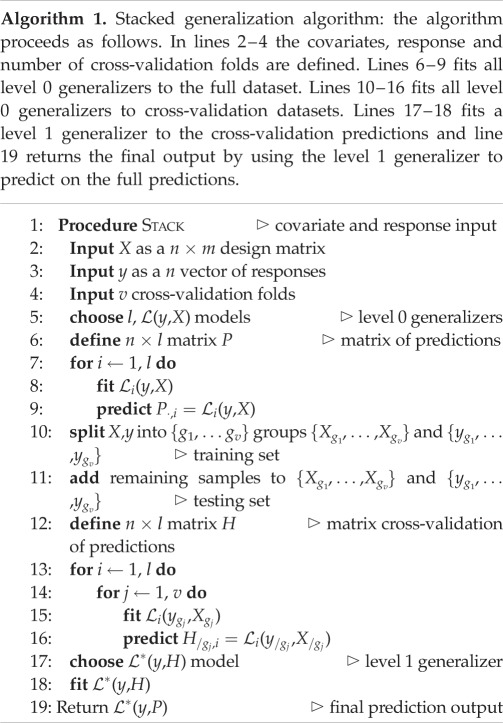
Abstract

Maps of infectious disease—charting spatial variations in the force of infection, degree of endemicity and the burden on human health—provide an essential evidence base to support planning towards global health targets. Contemporary disease mapping efforts have embraced statistical modelling approaches to properly acknowledge uncertainties in both the available measurements and their spatial interpolation. The most common such approach is Gaussian process regression, a mathematical framework composed of two components: a mean function harnessing the predictive power of multiple independent variables, and a covariance function yielding spatio-temporal shrinkage against residual variation from the mean. Though many techniques have been developed to improve the flexibility and fitting of the covariance function, models for the mean function have typically been restricted to simple linear terms. For infectious diseases, known to be driven by complex interactions between environmental and socio-economic factors, improved modelling of the mean function can greatly boost predictive power. Here, we present an ensemble approach based on stacked generalization that allows for multiple nonlinear algorithmic mean functions to be jointly embedded within the Gaussian process framework. We apply this method to mapping Plasmodium falciparum prevalence data in sub-Saharan Africa and show that the generalized ensemble approach markedly outperforms any individual method.

1. Introduction

Author summary. Infectious disease mapping provides a powerful synthesis of evidence in an effective, visually condensed form. With the advent of new web-based data sources and systematic data collection in the form of cross-sectional surveys and health facility reporting, there is high demand for accurate methods to predict spatial maps. The primary technique used in spatial mapping is known as Gaussian process regression (GPR). GPR is a flexible stochastic model that allows the modelling of disease-driving factors such as the environment while also capturing unknown residual spatial correlations in the data. We introduce a method that blends state-of-the-art machine learning methods with GPR to produce a model that substantially outperforms other methods commonly used in disease mapping. The utility of this new approach also extends far beyond just mapping and can be used for general machine learning applications across computational biology, including Bayesian optimization and mechanistic modelling.

Infectious disease mapping with model-based geostatistics [1] can provide a powerful synthesis of the available evidence base to assist surveillance systems and support progress towards global health targets, revealing the geographical bounds of disease occurrence and the spatial patterns of transmission intensity and clinical burden. A recent review found that, out of 174 infectious diseases with a strong rational for mapping, only seven (4%) have thus far been comprehensively mapped [2]. The primary factor impeding progress is a lack of accurate, population representative, geopositioned data. In recent years, this has begun to change as increasing volumes of spatially referenced data are collected from both cross-sectional household surveys and web-based data sources (e.g. Health Map [3]), bringing new opportunities for scaling up the global mapping of diseases. Alongside this surge in new data, novel statistical methods are needed that can generalize to new data accurately while remaining computationally tractable on large datasets. In this paper, we will introduce one such method designed with these aims in mind.

Owing to both a long history of published research in the field and a widespread appreciation among endemic countries for the value of cross-sectional household surveys as guides to intervention planning, malaria is an example of a disease that has been comprehensively mapped. Over the past decade, volumes of publicly available malaria prevalence data—defined as the proportion of parasite positive individuals in a sample—have reached sufficiency to allow for detailed spatio-temporal mapping [4]. From a statistical perspective, the methodological mainstay of these malaria prevalence mapping efforts has been GPR [5–8]. Gaussian processes are a flexible semi-parametric regression technique defined entirely through a mean function, μ( · ), and a covariance function, k( · , · ). The mean function models an underlying trend, such as the effect of environmental/socio-economic factors, while the covariance function applies Bayesian shrinkage to residual variation from the mean such that points close to each other in space and time tend towards similar values. The resulting ability of Gaussian processes to strike a parsimonious balance in the weighting of explained and unexplained spatio-temporal variation has led to their near exclusive use in contemporary studies of the geography of malaria prevalence [1,4,7–10].

Outside of disease mapping, Gaussian processes have been used for numerous applications in machine learning, including regression [1,5,6], classification [5] and optimization [11]; their popularity leading to the development of efficient computational techniques and statistical parametrizations. A key challenge for the implementation of Gaussian process models arises in the statistical learning (or inference) of the underlying parameters controlling the chosen mean and covariance functions. Learning is typically performed using Markov chain Monte Carlo (MCMC) or by maximizing the marginal likelihood [5], both of which are made computationally demanding by the need to compute large matrix inverses returned by the covariance function. The complexity of this inverse operation is in computation and in storage in the naive case [5], which imposes practical limits on data sizes [5]. MCMC techniques may be further confounded by mixing problems in the Markov chains. These challenges have necessitated the use of highly efficient MCMC methods, such as Hamiltonian MCMC [12] or posterior approximation approaches, such as the integrated nested Laplace approximation [13], expectation propagation [5,14,15] and variational inference [16,17]. Additionally, many frequentist approaches have been developed including matrix free [18] and primal learning approaches [19]. Many of these methods adopt finite-dimensional representations of the covariance function yielding sparse precision matrices, either by specifying a fully independent training conditional structure [20] or by identifying a Gaussian Markov random field approximation to the continuous process [21].

Alongside these improved methods for inference, recent research has focussed on model development to increase the flexibility and diversity of parametrizations for the covariance function, with new techniques using solutions to stochastic partial differential equations (allowing for easy extensions to non-stationary and anisotropic forms [21]), the combination of kernels additively and multiplicatively [22], and various spectral representations [23].

One aspect of Gaussian processes that has remained largely neglected is the mean function which is often—and indeed with justification in some settings—simply set to zero and ignored. However, in the context of disease mapping, where the biological phenomena are driven by a complex interplay of environmental and socio-economic factors [24], the mean plays a central role in improving the predictive performance of Gaussian process models. Furthermore, it has also been shown that using a well-defined mean function can allow for simpler covariance functions (and hence simpler, scalable inference techniques) [25].

The steady growth of remotely sensed data with incredible spatio-temporal richness [24] combined with well-developed biological models [26] has meant that there is a rich suite of environmental and socio-economic covariates currently available. In previous malaria mapping efforts, these covariates have been modelled as simple linear predictors [7–9] that fail to capture complex nonlinearities and interactions, leading to a reduced overall predictive performance. Extensive covariate engineering can be performed by introducing large sets of nonlinear and interacting transforms of the covariates, but this brute force combinatorial problem quickly becomes computationally inefficient [4,24].

In the field of machine learning and data science, there has been great success with algorithmic approaches that neglect the covariance and focus on learning from the covariates alone [27,28]. These include tree-based algorithms such as boosting [29] and random forests [30], generalized additive spline models [31,32], multivariate adaptive regression splines [33] and regularized regression models [34]. The success of these methods is grounded in their ability to manipulate the bias–variance trade-off [35], capture interacting nonlinear effects and perform automatic covariate selection. The technical challenges of hierarchically embedding these algorithmic methods within the Gaussian process framework are forbidding and many of the approximation methods that make Gaussian process models computationally tractable would struggle with their inclusion. Furthermore, it is unclear which of these approaches would best characterize the mean function when applied across different diseases and settings. In this paper, we propose a simplified embedding method based on stacked generalization [36,37] that focuses on improving the mean function of a Gaussian process, thereby allowing for substantial improvements in the predictive accuracy beyond what has been achieved in the past.

2. Material and methods

2.1. Gaussian process regression

We define our response, y_s,t = {y_(s,t)[1], …, y_(s,t)[n]}, as a vector of n empirical logit transformed malaria prevalence surveys at location–time pairs, (s, t)[i], with X_s,t = {(x_1:m)[1], …, (x_1:m)[n]} denoting a corresponding n × m design matrix of m covariates (see section ‘Data, covariates and experimental design’). The likelihood of the observed response is 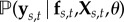, which we will write simply as , suppressing the spatio-temporal indices for ease of notation. Naturally, f(s, t) [= f_s,t] is the realization of a Gaussian process with mean function, μ_θ( · ), and covariance function, k_θ( · , · ), controlled by elements of a low-dimensional vector of hyperparameters, θ. Formally, the Gaussian process is defined as an (s, t)-indexed stochastic process for which the joint distribution over any finite collection of points, (s, t)[i], is multivariate Gaussian with mean vector, μ_i = m((s, t)[i] | θ), and covariance matrix, Σ_i,j = k((s, t)[i], (s, t)[j] | θ). The Bayesian hierarchy is completed by defining a vector of prior distributions for θ, which may potentially include hyperparameters for the likelihood (e.g. overdispersion in a β-binomial) in addition to those on parametrizing the mean and covariance functions, e.g. the mean function coefficients β. In hierarchical notation, supposing for clarity an independent and identically distributed (iid) normal likelihood with variance, σ²_e:

2.1

Following Bayes theorem the posterior distribution resulting from this hierarchy becomes

2.2

where the denominator in equation (2.2) is the marginal likelihood, .

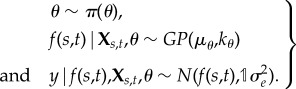
Given the hierarchical structure in equation (2.1) and the conditional properties of Gaussian distributions, the conditional predictive distribution for the mean of observations, z [= z_s′,t′], at location–time pairs, (s′, t′)[j], for a given θ is also Gaussian with the form

2.3

and

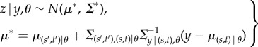
2.4

where . For specific details on the parametrization of Σ, see the appendix

When examining the conditional expectation in equation (2.4) and splitting the summation into terms μ_{(s′,t′) |θ} and Σ_{(s′,t′),(s,t) |θ}Σ⁻¹_y|(s,t),θ(y − μ_{(s,t) |θ}), it is clear that the first specifies a global underlying mean, while the second augments the residuals from that mean by the covariance function. Clearly, if the mean function fits the data perfectly, the covariance in the second term of the expectation would drop out and, conversely, if the mean function is zero, then only the covariance function would model the data. This expectation therefore represents a balance between the underlying trend and the residual correlated noise.

In most applications of GPR, a linear mean function (μ_θ = X_s,tβ) is used, where β is a vector of m coefficients. However, when a rich suite of covariates is available, this linear mean may be suboptimal, limiting the generalization accuracy of the model. To improve on the linear mean, covariate basis terms can be expanded to include parametric nonlinear transforms and interactions, but finding the optimal set of basis is computationally demanding and often leaves the researcher open to data snooping [38]. In this paper, we propose using an alternative two-stage statistical procedure to first obtain a set of candidate nonlinear mean functions using multiple different algorithmic methods fit without reference to the assumed spatial covariance structure and then include those means in the Gaussian process via stacked generalization.

2.2. Stacked generalization

Stacked generalization [36], also called stacked regression [37], is a general ensemble approach to combining different models. In brief, stacked generalizers combine different models together to produce a meta-model with equal or better predictive performance than the constituent parts [39]. In the context of malaria mapping, our goal is to fuse multiple algorithmic methods with GPR to both fully exploit the information contained in the covariates and model spatio-temporal correlations.

To present stacked generalization, we begin by introducing standard ensemble methods and show that stacked generalization is simply a special case of this powerful technique. To simplify notation, we suppress the spatio-temporal index and dependence on θ. Consider models, with outputs . The choice of these models is described in the electronic supplementary material. We denote the true target function as f(x) and can therefore write the regression equation as y_i(x) = f(x) + ε_i(x). The average sum-of-squares error for model i is defined as . Our goal is to estimate an ensemble model across all models, denoted as . The simplest choice for C is an average across all models . However, this average assumes that the error of all models are the same, and that all models perform equally well. The assumption of equal performance may hold when using variants of a single model (i.e. bagging) but is unsuitable when very different models are used. Therefore, a simple extension would be to use a weighted mean across models subject to constraints (convex combinations). These constraints prevent extreme predictions in well-predicting models and impose the sensible inequality 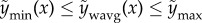[37]. The optimal βs can be found by quadratic programming or by Bayesian linear regression with a Dirichlet/categorical prior on the coefficients. One particularly interesting result of combining models using this constrained weighted mean is the resulting decomposition of error into two terms [40]

2.5

The above equation is a reformulation of the standard bias–variance decomposition [35] where the first term describes the average error of all models and the second (termed the ambiguity) is the spread of each member of the ensemble around the weighted mean, measuring the disagreement among models. Equation (2.5) shows that combining multiple models with low error but with large disagreements produces a lower overall error. It should be noted that equation (2.5) makes the assumption that y(x) = f(x).

Combination of models in an ensemble as described above can potentially lead to reductions in errors. However, the ensemble models introduced so far are based only on training data and therefore neglect the issue of model complexity and tell us nothing about the ability to generalize to new data. To state this differently, the constrained weighted mean model will always allocate the highest weight to the model that most over fits the data. The standard method of addressing this issue is to use cross-validation as a measure of the generalization error and select the best performing of the models. Stacked generalization provides a technique to combine the power of ensembles described above but also produces models that can generalize well to new data. The principle idea behind stacked generalization is to train models (termed level 0 generalizers) and generalize their combined behaviour via a second model (termed the level 1 generalizer). Practically this is done by specifying a K-fold cross-validation set, training all level 0 models on these sets and using the cross-validation predictions to train a level 1 generalizer. This calibrates the level 1 model based on the generalization ability of the level 0 models. After this level 1 calibration, all level 0 models are refitted using the full dataset and these predictions are used in the level 1 model without refitting. (This procedure is more fully described in algorithm 1 and the schematic design shown in the electronic supplementary material.) The combination of ensemble modelling with the ability to generalize well has made stacking one of the best methods to achieve state-of-the-art predictive accuracy [37,39,41].

Defining the most appropriate level 1 generalizer based on a rigorous optimality criterion is still an open problem, with most applications using the constrained weighted mean specified above [37,39]. Using the weighted average approach can be seen as a general case of cross-validation, where standard cross-validation would select a single model by specifying a single β_i as 1 and all other β_is as zero. Additionally, it has been shown that using the constrained weighted mean method will perform asymptotically as well as be the best possible choice among the family of weight combinations [39].

Here, we suggest using GPR as the level 1 generalizer. Revisiting equation (2.3), we can replace μ_{(s′,t′) |θ} with a linear stacked function 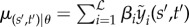across level 0 generalizers, where the subscript denotes predictions from the ith level 0 generalizer (see algorithm 1). We also impose inequality constraints on β_i such that 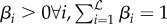. This constraint allows the βs to approximately sum to one and helps computational tractability. It should be noted that empirical analysis suggests that simply imposing β_i > 0∀i is practically sufficient [37].

The intuition in this extended approach is that the stacked mean of the Gaussian process uses multiple different methods to exploit as much predictive capacity from the covariates as possible and then leaves the spatio-temporal residuals to be captured through the Gaussian process covariance function. In the electronic supplementary material, we prove that this approach yields all the benefits of using the constrained weighted mean (equation (2.5)) but allows for a further reduction in overall error from the covariance function of the Gaussian process.

We note here that that stacked generalizers are distinct from Bayesian model averaging (BMA). Stacked generalizers expand and change the hypothesis space from which the learning algorithm chooses a function (e.g. from single decision trees to a linear combination of them) and can take a variety of different forms. BMA, however, weights hypotheses from the original space according to a fixed formula [42]. Owing to these fundamental differences, previous studies have suggested that the stacking has better robustness properties than BMA in the most important settings [43].

2.3. Data, covariates and experimental design

The hierarchical structure most commonly used in infectious disease mapping is that shown in equation (2.1). In malaria studies, our response data are discrete random variables representing the number of individuals testing positive for the Plasmodium falciparum malaria parasite, N⁺, out of the total number tested, N, at a given location. If the response is aggregated from the individual household level to a cluster or enumeration area level, the centroid of the component sites is used as the spatial position datum. The ratio of N⁺ to N is defined as the parasite rate or prevalence and is a key epidemiological parameter measuring transmission intensity. The response data were additionally transformed via the empirical logit [1,4]. Pre-modelling standardization of the available prevalence data for age and diagnostic type has also been performed on the data used here, as described in depth in [4,7]. Our analysis is performed over sub-Saharan Africa with the study area and dataset partitioned into four epidemiologically distinct regions [7]—eastern Africa, western Africa, north eastern Africa and southern Africa—each of which was modelled separately (figure 1). The data used in this study are identical to that recently published by Bhatt et al. [4], and the collection process has been described in detail previously [4,7,8].

Figure 1.

(a) Plot of the 23 131 prevalence surveys conducted between 2000 and 2015. The survey data are age and diagnostic standardized and presented as a continuum of blue to red from 0 to 1. (b) Study area of stable malaria transmission in sub-Saharan Africa. Our analysis was performed on four zones—western Africa, north eastern Africa, eastern Africa and southern Africa

All the malaria response data are freely available through an online data explorer portal found at http://www.map.ox.ac.uk/. All the covariate grids are freely available and can be accessed at https://earthengine.google.com/datasets/. The code used in this analysis is freely available at https://codeshare.io/5wnRn7. Fitting and analysis was performed in the R programming language using the INLA, H2O, mgcv and Earth packages. More information can be found in the electronic supplementary material.

The covariates (i.e. independent variables) used in this research consist of raster layers spanning the entire continent at a 2.5 arc-min (5 km × 5 km) spatial resolution. The majority of these raster covariates were derived from high temporal resolution satellite images that were first gap-filled [44] to eliminate missing data (resulting primarily from persistent cloud cover over equatorial forests) and then aggregated to create a dynamic (i.e. temporally varying) dataset for every month throughout the study period (2000–2015). The list of covariates is presented in table 1 and detailed information on individual covariates can be found here [24,26,44]. The set of monthly dynamic covariates was further expanded to include lagged versions of the covariate at two-month, four-month and six-month lags. The main objective of this study was to judge the predictive performance of the various generalization methods and therefore no variable selection or thinning of the covariate set was performed. It should be noted, however, that many of the level 0 generalizers performed variable selection automatically (e.g. elastic net regression).

Table 1.

List of environmental, socio-demographic and land type covariates used.

variable class	variable(s) source type
temperature	land surface temperature (day, night and diurnal-flux)	MODIS product	dynamic monthly
temperature suitability	temperature suitability for P. falciparum	modelled product	dynamic monthly
precipitation	mean annual precipitation	WorldClim	synoptic
vegetation vigour	enhanced vegetation index	MODIS derivative	dynamic monthly
surface wetness	tasselled cap wetness	MODIS derivative	dynamic monthly
surface brightness	tasselled cap brightness	MODIS derivative	dynamic monthly
IGBP landcover	fractional landcover	MODIS product	dynamic annual
IGBP landcover pattern	landcover patterns	MODIS derivative	dynamic annual
terrain steepness	SRTM derivatives	MODIS product	static
flow & topographic wetness	topographically redistributed water	SRTM derivatives	static
elevation	digital elevation model	SRTM	static
human population	AfriPop	modelled products	dynamic annual
infrastructural development	accessibility to urban centres and night-time lights	modelled product and VIIRS	static
moisture metrics	aridity and potential evapotranspiration	modelled products	synoptic

The resolution used throughout was defined by the covariate grids at 5 km × 5 km. The prevalence points were therefore snapped to the centroid of the pixel containing them. If multiple cluster points were contained within the same pixel at the same time, then they were aggregated. Likewise, the spatial field, which can be projected or evaluated at any spatial resolution, was taken as the value of the spatial field at the centroid of the pixel.

The level 0 generalizers used were gradient-boosted trees [29,45], random forests [30], elastic net regularized regression [34], generalized additive splines [27,32] and multivariate adaptive regression splines [33]. The level 1 generalizers used were stacking using a constrained weighted mean and stacking using GPR. We also fitted a standard Gaussian process for benchmark comparisons with the level 0 and 1 generalizers. Stacked fitting was performed following algorithm 1. Full analysis and K-fold cross-validation was performed five times and then averaged to reduce any bias from the choices of cross-validation set. The averaged cross-validation results were used to estimate the generalization error by calculating the mean squared error (MSE (y − f)²)), mean absolute error (MAE|y − f|) and the correlation.

3. Results

The results of our analysis are summarized in figure 2, where pairwise comparisons of MSE versus MAE versus correlation are shown. Across the eastern, southern and western African regions (figure 2a,b,d), we found a consistent ranking pattern in the generalization performance with the stacked Gaussian process approach presented in this paper outperforming all other methods. The constrained weighted mean stacked approach was the next best method followed by the standard Gaussian process (with a linear mean) and gradient-boosted trees. Random forests, multivariate adaptive regression splines and generalized additive splines all had similar performance, and the worst performing method was the elastic net regularized regression. For the north eastern region (figure 2c), again the stacked Gaussian process approach was the best performing method but the standard Gaussian process performed better than the constrained weighted mean stacked approach, though only in terms of MAE and MSE.

Figure 2.

Comparisons of cross-validation MSE versus MAE versus correlation. Level 1 generalizers and the standard Gaussian process are shown in blue and all level 0 generalizers are shown in red. SGP, stacked Gaussian process; CWM, stacked constrained weighted mean; GP, standard Gaussian process; GBM, gradient-boosted trees; GAS, generalized additive splines; FR, random forests; MARS, multivariate adaptive regression splines and LIN, elastic net regularized linear regression. (a) Eastern Africa, (b) southern Africa, (c) north eastern Africa and (d) western Africa. (Online version in colour.)

One average, across all regions, the stacked Gaussian process approach reduced the MAE and MSE by 9% (1–13%) (values in parentheses are the minimum and maximum across all regions) and 16% (2–24%), respectively, and increased the correlation by 3% (1–5%) over the next best constrained weighted mean approach, thereby empirically reinforcing the theoretical bounds derived in the electronic supplementary material proof. When compared with the widely used elastic net linear regression, the relative performance increase of the Gaussian process stacked approach is stark, with reduced MAE and MSE of 25% (12–33%) and 25% (19–30%), respectively, and increase in correlation by 39% (20–50%).

Compared to the standard Gaussian process previously used in malaria mapping, the stacked Gaussian process approach reduced MAE and MSE by 10% (3–14%) and 18% (9–26%), respectively, and increased the correlation by 6% (3–7%).

Consistently across all regions, the best non-stacked method was the standard Gaussian process with a linear mean function. Of the level 0 generalizers gradient-boosted trees were the best performing method, with performance close to that of the standard Gaussian process. The standard Gaussian process only had a modest improvement over gradient-boosted trees with average reductions in MAE and MSE of 4% (1–8%) and 7% (1–13%), respectively, and increases in correlation of 3% (1–7%).

Figure 3 shows the predicted map for all level 0 generalizers and the stacked Gaussian process approach for 2011 in the eastern Africa region. There are clear similarities in the high and low regions across all maps and a strong correspondence to previous approaches [4,7,8]. The final ensemble map can be seen as a consensus of the individual level 0 maps where the stacking algorithm weights each map according to generalization performance. This is why the final stacked Gaussian process map most resembles the gradient-boosted tree approach (the best predicting method; figure 2a) as opposed to the elastic net regularized linear regression approach (the worst predicting method). However, some idiosyncrasies of the gradient-boosted approach, such as the sharp transition line in southern Tanzania, are corrected in the stacked Gaussian process approach owing to the other level 0 methods and the addition of spatio-temporal correlation.

Figure 3.

Predicted prevalence maps for eastern Africa in 2011 for gradient-boosted trees (GBM), random forests (FR), elastic net regularized linear regression (LIN), multivariate adaptive regression splines (MARS), generalized additive splines (GAS) and the new stacked Gaussian process (SGP).

4. Discussion

All the level 0 generalization methods used in this paper have been previously applied to a diverse set of machine learning problems and have track records of good generalizability [27]. For example, in closely related ecological applications, these level 0 methods have been shown to far surpass classical learning approaches [46]. However, as introduced by Wolpert [36], rather than picking one level 0 method, an ensemble via a second generalizer has the ability to improve prediction beyond that achievable by the constituent parts [40]. Indeed, in all previous applications [36,37,39,47] ensembling by stacking has consistently produced the best predictive models across a wide range of regression and classification techniques. The most popular level 1 generalizer is the constrained weighted mean with convex combinations. The key attraction of this level 1 generalizer is the ease of implementation and theoretical properties [39,40]. In this paper, we show that, for disease mapping, stacking using Gaussian processes is more predictive and generalizes better than both single level 0 generalizers in isolation and the more common stacking approach using a constrained weighted mean.

The key benefit of stacking is summarized in equation (2.5) where the total error of an ensemble model can be reduced by using multiple, very different, but highly predictive models. However, stacking using a constrained weighted mean only ensures that the predictive power of the covariates are fully used and does not exploit the predictive power that could be gained from characterizing any residual covariance structure. The standard Gaussian process suffers from the inverse situation where the covariates are underexploited and predictive power is instead gained from leveraging residual spatio-temporal covariance. In a standard Gaussian process, the mean function is usually paramaterized through simple linear basis functions [48] that are often unable to model the complex nonlinear interactions needed to correctly capture the true underlying mean. This inadequacy is best highlighted by the poor generalization performance of the elastic net regularized regression method across all regions. The trade-off between the variance explained by the covariates versus that explained by the covariance function will undoubtedly vary from setting to setting. For example, in the eastern, southern and western African regions, the constrained weighted mean stacking approach performs better than the standard Gaussian process and the level 0 gradient-boosted trees generalizer performs almost as well as the standard Gaussian process. For these regions, this shows a strong influence of the covariates on the underlying process. By contrast, for the north eastern African region, the standard Gaussian process does better than both the constrained weighted mean approach (in terms of error not correlation) and all of the level 0 generalizers, suggesting a weak influence of the covariates. However, for all zones, the stacked Gaussian process approach is consistently the best approach across all predictive metrics. By combining both the power of Gaussian processes to characterize a complex covariance structure, and multiple algorithmic approaches to fully exploit the covariates, the stacked Gaussian process approach combines the best of both worlds and predicts well in all settings.

This paper introduces one way of stacking that is tailored for spatio-temporal data. However, the same principles are applicable to purely spatial or purely temporal data, settings in which Gaussian process models excel. Additionally, there is no constraint on the types of level 0 generalizers that can be used; dynamical models of disease transmission, e.g. Malaria mechanistic models [49,50] can be fitted to data and used as the mean function within the stacked framework. Using dynamical models in this way can constrain the mean to include known biological mechanisms that can potentially improve generalizability, allow for forecast predictions and help restrict the model to only plausible functions when data are sparse. Finally, multiple different stacking schemes can be designed (see the electronic supplementary material for details) and relaxations on linear combinations can be implemented [47].

Gaussian processes are increasingly being used for expensive optimization problems [51] and Bayesian quadrature [52]. In current implementations, both of these applications are limited to low-dimensional problems typically with less than 10 parameters. Future work will explore the potential for stacking to extend these approaches to high-dimensional settings. The intuition is that the level 0 generalizers can accurately and automatically learn much of the latent structure in the data, including complex features like non-stationarity, which are a challenge for Gaussian processes. Learning this underlying structure through the mean can leave a much simpler residual structure [25] to be modelled by the level 1 Gaussian process.

In this paper, we have focused primarily on prediction, that is neglecting any causal inference and only searching for models with the lowest generalization error. Determining causality from the complex relationships fitted through the stacked algorithmic approaches is difficult, but empirical methods such as partial dependence [29] or individual conditional expectation [53] plots can be used to approximate the marginal relationships from the various covariates. Similar statistical techniques can also be used to determine covariate importance.

Increasing volumes of data and computational capacity afford unprecedented opportunities to scale up infectious disease mapping for public health uses [54]. Maps of diseases and socio-economic indicators are increasingly being used to inform policy [4,55], creating demand for methods to produce accurate estimates at high spatial resolutions. Many of these maps can subsequently be used in other models but, in the first instance, creating these maps requires continuous covariates, the bulk of which come from remotely sensed sources. For many indicators, such as HIV or tuberculosis, these remotely sensed covariates serve as proxies for complex phenomenan and as such, the simple mean functions in standard Gaussian processes are insufficient to predict with accuracy and low generalization error. The stacked Gaussian process approach introduced in this paper provides an intuitive, easy-to-implement method that predicts accurately through exploiting information in both the covariates and covariance structure.

Data accessibility

All the data used in this paper are freely accessible. All the malaria response data are freely available through an online data explorer portal found at http://www.map.ox.ac.uk/. All the covariate grids are freely available and can be accessed at https://earthengine.google.com/datasets/. The code used in this analysis is freely available at https://codeshare.io/5wnRn7. Fitting and analysis was performed in the R programming language using the INLA, H2O, mgcv and Earth packages. More information can be found in the electronic supplementary material.

Authors' contributions

S.B. conceived of and designed the research. S.B. and E.C. drafted the manuscript. S.B. drafted the electronic supplementary material and conducted the analyses. D.J.W. prepared data. S.B., E.C. and S.R.F. supported the analyses. D.L.S. and P.W.G. supported interpretation and policy contextualization. All authors discussed the results and contributed to the revision of the final manuscript.

Competing interests

We declare we have no competing interests.

Funding

S.B. is supported by the MRC Outbreak Centre and the Bill and Melinda Gates Foundation (OPP1152978). D.L.S. was supported by the Bill and Melinda Gates Foundation (OPP1110495), National Institutes of Health/National Institute of Allergy and Infectious Diseases (U19AI089674), and the Research and Policy for Infectious Disease Dynamics (RAPIDD) programme of the Science and Technology Directorate, Department of Homeland Security, and the Fogarty International Center, National Institutes of Health. P.W.G. is a Career Development Fellow (K00669X) jointly funded by the UK Medical Research Council (MRC) and the UK Department for International Development (DFID) under the MRC/DFID Concordat agreement, also part of the EDCTP2 programme supported by the European Union, and receives support from the Bill and Melinda Gates Foundation (OPP1068048, OPP1106023). These grants also support D.J.W. and E.C.

References

- 1.Diggle P, Ribeiro PJ. 2007. Model-based geostatistics. New York, NY: Springer. [Google Scholar]
- 2.Hay SI. 2013. Global mapping of infectious disease. Phil. Trans. R. Soc. B 368, 20120250 ( 10.1098/rstb.2012.0250) [DOI] [PMC free article] [PubMed] [Google Scholar]
- 3.Freifeld CC, Mandl KD, Reis BY, Brownstein JS. 2008. HealthMap: global infectious disease monitoring through automated classification and visualization of Internet media reports. J. Am. Med. Inform. Assoc. 15, 150–157. ( 10.1197/jamia.M2544) [DOI] [PMC free article] [PubMed] [Google Scholar]
- 4.Bhatt S, et al. 2015. The effect of malaria control on Plasmodium falciparum in Africa between 2000 and 2015. Nature 526, 207–211. ( 10.1038/nature15535) [DOI] [PMC free article] [PubMed] [Google Scholar]
- 5.Rasmussen CE, Williams CKI. 2006. Gaussian processes for machine learning, vol. 14 Cambridge, MA: The MIT Press. [Google Scholar]
- 6.Bishop CM. 2006. Pattern recognition and machine learning, vol. 4 London, UK: Springer. [Google Scholar]
- 7.Gething PW, Patil AP, Smith DL, Guerra CA, Elyazar IRF, Johnston GL, Tatem AJ, Hay SI. 2011. A new world malaria map: Plasmodium falciparum endemicity in 2010. Malar. J. 10, 378 ( 10.1186/1475-2875-10-378) [DOI] [PMC free article] [PubMed] [Google Scholar]
- 8.Hay SI, et al. 2009. A world malaria map: Plasmodium falciparum endemicity in 2007. PLoS Med. 6, 0286–0302. ( 10.1371/annotation/a7ab5bb8-c3bb-4f01-aa34-65cc53af065d) [DOI] [PMC free article] [PubMed] [Google Scholar]
- 9.Gosoniu L, Msengwa A, Lengeler C, Vounatsou P. 2012. Spatially explicit burden estimates of malaria in Tanzania: Bayesian geostatistical modeling of the malaria indicator survey data. PLoS ONE 7, e23966 ( 10.1371/journal.pone.0023966) [DOI] [PMC free article] [PubMed] [Google Scholar]
- 10.Adigun AB, Gajere EN, Oresanya O, Vounatsou P. 2015. Malaria risk in Nigeria: Bayesian geostatistical modelling of 2010 malaria indicator survey data. Malar. J. 14, 156 ( 10.1186/s12936-015-0683-6) [DOI] [PMC free article] [PubMed] [Google Scholar]
- 11.Snoek J, Larochelle H, Adams RP. 2012. Practical Bayesian optimization of machine learning algorithms. Adv. Neural Inf. Process. Syst. 25, 2951–2959. [Google Scholar]
- 12.Hoffman MD, Gelman A. 2014. The no-U-turn sampler: adaptively setting path lengths in Hamiltonian Monte Carlo. J. Mach. Learn. Res. 15, 1593–1623. [Google Scholar]
- 13.Rue H, Martino S, Chopin N. 2009. Approximate Bayesian inference for latent Gaussian models by using integrated nested Laplace approximations. J. R. Stat. Soc. Ser. B (Stat. Methodol.) 71, 319–392. ( 10.1111/j.1467-9868.2008.00700.x) [DOI] [Google Scholar]
- 14.Vanhatalo J, Pietiläinen V, Vehtari A. 2010. Approximate inference for disease mapping with sparse Gaussian processes. Stat. Med. 29, 1580–1607. ( 10.1002/sim.3895) [DOI] [PubMed] [Google Scholar]
- 15.Minka TP. 2001. Expectation propagation for approximate Bayesian inference. In Proceedings of the Seventeenth conference on Uncertainty in artificial intelligence, pp. 362–369. Burlington, MA: Morgan Kaufmann Publishers. [Google Scholar]
- 16.Hensman J, Fusi N, Lawrence ND. 2013. Gaussian processes for big data. ArXiv 1309.6835. (http://arxiv.org/abs/1309.6835)
- 17.Opper M, Archambeau C. 2009. The variational Gaussian approximation revisited. Neural Comput. 21, 786–792. ( 10.1162/neco.2008.08-07-592) [DOI] [PubMed] [Google Scholar]
- 18.Dutta S, Mondal D. 2016. REML estimation with intrinsic Matérn dependence in the spatial linear mixed model. Electron. J. Stat. 10, 2856–2893. ( 10.1214/16-EJS1125) [DOI] [Google Scholar]
- 19.Rahimi A, Recht B. 2008. Random features for large-scale kernel machines. Adv. Neural Inf. Process. Syst. 20, 1177–1184. [Google Scholar]
- 20.Quiñonero-Candela J, Rasmussen CE. 2005. A unifying view of sparse approximate Gaussian process regression. J. Mach. Learn. Res. 6, 1939–1959. [Google Scholar]
- 21.Lindgren F, Rue H, Lindström J. 2011. An explicit link between Gaussian fields and Gaussian Markov random fields: the stochastic partial differential equation approach. J. R. Stat. Soc. Ser. B (Stat. Methodol.) 73, 423–498. ( 10.1111/j.1467-9868.2011.00777.x) [DOI] [Google Scholar]
- 22.Duvenaud D, Lloyd JR, Grosse R, Tenenbaum JB, Ghahramani Z. 2013. Structure discovery in nonparametric regression through compositional kernel search. ArXiv 1302.4922. (http://arxiv.org/abs/1302.4922)
- 23.Wilson AG, Adams RP. 2013. Gaussian process kernels for pattern discovery and extrapolation. ArXiv 1302.4245. (http://arxiv.org/abs/1302.4245)
- 24.Weiss DJJ, Mappin B, Dalrymple U, Bhatt S, Cameron E, Hay SII, Gething PWW. 2015. Re-examining environmental correlates of Plasmodium falciparum malaria endemicity: a data-intensive variable selection approach. Malar. J. 14, 68 ( 10.1186/s12936-015-0574-x) [DOI] [PMC free article] [PubMed] [Google Scholar]
- 25.Fuglstad G-A, Simpson D, Lindgren F, Rue H. 2015. Does non-stationary spatial data always require non-stationary random fields? Spat. Stat. 14, 505–531. ( 10.1016/j.spasta.2015.10.001) [DOI] [Google Scholar]
- 26.Weiss DJJ, Bhatt S, Mappin B, VanBoeckel TPP, Smith DLL, Hay SII, Gething PWW. 2014. Air temperature suitability for Plasmodium falciparum malaria transmission in Africa 2000–2012: a high-resolution spatiotemporal prediction. Malar. J. 13, 171 ( 10.1186/1475-2875-13-171) [DOI] [PMC free article] [PubMed] [Google Scholar]
- 27.Hastie T, Tibshirani R, Friedman JH. 2009. The elements of statistical learning. Berlin, Germany: Springer. [Google Scholar]
- 28.Caruana R, Niculescu-Mizil A. 2006. An empirical comparison of supervised learning algorithms. In Proc. of the 23rd Int. Conf. on Machine Learning, pp. 161–168. New York, NY: ACM. [Google Scholar]
- 29.Friedman JH. 2001. Greedy function approximation: a gradient boosting machine. Ann. Stat. 29, 1189–1232. ( 10.1214/aos/1013203451) [DOI] [Google Scholar]
- 30.Breiman L. 2001. Random forests. Mach. Learn. 45, 5–32. ( 10.1023/A:1010933404324) [DOI] [Google Scholar]
- 31.Tibshirani R, Hastie T. 1986. Generalized additive models. Stat. Sci. 1, 297–310. ( 10.1214/ss/1177013604) [DOI] [PubMed] [Google Scholar]
- 32.Wood S. 2006. Generalized additive models: an introduction with R. Boca Raton, FL: CRC Press. [Google Scholar]
- 33.Friedman JH. 1991. Multivariate adaptive regression splines. Ann. Stat. 19, 1–67. ( 10.1214/aos/1176347963) [DOI] [PubMed] [Google Scholar]
- 34.Zou H, Hastie T. 2005. Regularization and variable selection via the elastic net. J. R. Stat. Soc. Ser. B (Stat. Methodol.). 67, 301–320. ( 10.1111/j.1467-9868.2005.00503.x) [DOI] [Google Scholar]
- 35.Geman S, Bienenstock E, Doursat R. 1992. Neural networks and the bias/variance dilemma. Neural Comput. 4, 1–58. ( 10.1162/neco.1992.4.1.1) [DOI] [Google Scholar]
- 36.Wolpert DH. 1992. Stacked generalization. Neural Netw. 5, 241–259. ( 10.1016/S0893-6080(05)80023-1) [DOI] [Google Scholar]
- 37.Breiman L. 1996. Stacked regressions. Mach. Learn. 24, 49–64. ( 10.1007/BF00117832) [DOI] [Google Scholar]
- 38.Abu-Mostafa YS, Magdon-Ismail M, Lin HT. 2012. Learning from data. Pasadena, CA: AMLBook. [Google Scholar]
- 39.van der Laan MJ, Polley EC, Hubbard AE. 2007. Super learner. Stat. Appl. Genet. Mol. Biol. 6, 25 ( 10.2202/1544-6115.1309) [DOI] [PubMed] [Google Scholar]
- 40.Krogh A, Vedelsby J. 1995. Neural network ensembles, cross validation, and active learning. Adv. Neural Inf. Process. Syst. 7, 231–238. [Google Scholar]
- 41.Puurula A, Read J, Bifet A. 2014. Kaggle LSHTC4 winning solution. ArXiv 1405.0546. (https://arxiv.org/abs/1405.0546. ) [Google Scholar]
- 42.Domingos P. 2012. A few useful things to know about machine learning. Commun. ACM 55, 78–87. ( 10.1145/2347736.2347755) [DOI] [Google Scholar]
- 43.Clarke B, Bertrand@stat Ubc Ca. 2003. Comparing Bayes model averaging and stacking when model approximation error cannot be ignored. J. Mach. Learn. Res. 4, 683–712. ( 10.1162/153244304773936090) [DOI] [Google Scholar]
- 44.Weiss DJ, Atkinson PM, Bhatt S, Mappin B, Hay SI, Gething PW. 2014. An effective approach for gap-filling continental scale remotely sensed time-series. ISPRS J. Photogramm. Remote Sens. 98, 106–118. ( 10.1016/j.isprsjprs.2014.10.001) [DOI] [PMC free article] [PubMed] [Google Scholar]
- 45.Friedman JH. 2002. Stochastic gradient boosting. Comput. Stat. Data Anal. 38, 367–378. ( 10.1016/S0167-9473(01)00065-2) [DOI] [Google Scholar]
- 46.Elith J, Leathwick JR, Hastie T. 2008. A working guide to boosted regression trees. J. Anim. Ecol. 77, 802–813. ( 10.1111/j.1365-2656.2008.01390.x) [DOI] [PubMed] [Google Scholar]
- 47.Sill J, Takacs G, Mackey L, Lin D. 2009. Feature-weighted linear stacking. ArXiv 0911.0460. (https://arxiv.org/pdf/0911.0460.pdf) [Google Scholar]
- 48.Rasmussen C. 2004. Gaussian processes in machine learning. In Advanced lectures on machine learning (eds Bousquet O, von Luxburg U, Rätsch G), pp. 63–71. Berlin, Germany: Springer. [Google Scholar]
- 49.Smith DL, McKenzie FE. 2004. Statics and dynamics of malaria infection in Anopheles mosquitoes. Malar. J. 3, 13 ( 10.1186/1475-2875-3-13) [DOI] [PMC free article] [PubMed] [Google Scholar]
- 50.Griffin JT, Ferguson NM, Ghani AC. 2014. Estimates of the changing age-burden of Plasmodium falciparum malaria disease in sub-Saharan Africa. Nat. Commun. 5, 3136 ( 10.1038/ncomms4136) [DOI] [PMC free article] [PubMed] [Google Scholar]
- 51.O'Hagan A. 1991. Bayes–Hermite quadrature. J. Stat. Plan. Inference 29, 245–260. ( 10.1016/0378-3758(91)90002-V) [DOI] [Google Scholar]
- 52.Hennig P, Osborne MA, Girolami M. 2015. Probabilistic numerics and uncertainty in computations. Proc. R. Soc. A 471, 20150142 ( 10.1098/rspa.2015.0142) [DOI] [PMC free article] [PubMed] [Google Scholar]
- 53.Goldstein A, Kapelner A, Bleich J, Pitkin E. 2015. Peeking inside the black box: visualizing statistical learning with plots of individual conditional expectation. J. Comput. Graph. Stat. 24, 44–65. ( 10.1080/10618600.2014.907095) [DOI] [Google Scholar]
- 54.Pigott DM, et al. 2015. Prioritising infectious disease mapping. PLoS Negl. Trop. Dis. 9, e0003756 ( 10.1371/journal.pntd.0003756) [DOI] [PMC free article] [PubMed] [Google Scholar]
- 55.Bhatt S, et al. 2013. The global distribution and burden of dengue. Nature 496, 504–507. ( 10.1038/nature12060) [DOI] [PMC free article] [PubMed] [Google Scholar]
Associated Data
This section collects any data citations, data availability statements, or supplementary materials included in this article.
Supplementary Materials
Data Availability Statement