Synchronous long-term oscillations in a synthetic gene circuit

Abstract

Synthetically engineered genetic circuits can perform a wide range of tasks but generally with lower accuracy than natural systems. Here we revisited the first synthetic genetic oscillator, the repressilator¹, and modified it based on principles from stochastic chemistry in single cells. Specifically, we sought to reduce error propagation and information losses, not by adding control loops, but by simply removing existing features. This created highly regular and robust oscillations. Some streamlined circuits kept 14 generation periods over a range of growth conditions and kept phase for hundreds of generations in single cells, allowing cells in flasks and colonies to oscillate synchronously without any coupling between them. Our results show that even the simplest synthetic genetic networks can achieve a precision that rivals natural systems, and emphasize the importance of noise analyses for circuit design in synthetic biology.

Many biological systems show remarkably precise and robust dynamics. For example, the circadian clock in cyanobacteria uses a combination of transcriptional and post-translational control mechanisms^{2, 3} to keep phase for weeks without entrainment, while displaying robustness to changes in temperature and growth rate^3–5. Synthetic circuits built from well-characterized parts can also exhibit a wide range of dynamical features – including arithmetic computations^{6, 7}, oscillations^{1, 8–13}, logic gates¹⁴ and edge detection¹⁵ – but often with lower accuracy. For example, the repressilator¹, a now iconic device that helped jump-start the field of synthetic biology 15 years ago, showed clear signs of oscillations using a simple design where three genes inhibit each other’s production in a single loop (A⊣B⊣C⊣A). However, only about 40% of cells were found to support oscillations, and those oscillations were quite irregular. Subsequent synthetic oscillators evaluated different control topologies or repression mechanisms^8–13, but most were again quite irregular in both phase and amplitude despite being mathematically designed to display sustained oscillations in a broad range of parameters.

The challenge when designing synthetic circuits to operate reliably in single cells is that biochemical noise can do more than just create different rate constants in different cells. On one hand, simple intrinsic noise can in principle enhance control¹⁶ and even create high-quality oscillations in systems that could not display limit cycles for any rate constants in the absence of noise^{17, 18}. On the other hand, any component present in low numbers can in principle randomize behavior of the whole system, and a single stochastic signaling step can introduce fundamental constraints¹⁹ that cannot be overcome by any control system. This suggests that simplicity could even help achieve accurate oscillations as long as stochastic effects are accounted for in the design, and that minimal control topologies may not only be elegant and interesting but also very effective. We therefore revisited the original repressilator to reduce error propagation from the reporter system, from core cellular processes, and from within the circuit itself.

The repressilator consists of three genes – tetR from the Tn10 transposon, cI from bacteriophage λ and lacI from the lactose operon – and each repressor has a C-terminal ssrA tag²⁰ that targets it for degradation (Fig. 1a). The whole circuit was encoded on a low-copy pSC101 plasmid in an Escherichia coli strain lacking lacI, and a second high-copy ColE1 reporter plasmid encoded GFP under the control of TetR with a modified degradation tag^{1, 21}. We first reevaluated this circuit using a microfluidic device in which cells are trapped in short channels and newborn cells are washed away by fresh medium^{22, 23} (Fig. 1a). Tracking reporter levels under the microscope for hundreds of consecutive generations across hundreds of single-cell traces (Methods) revealed clear oscillatory dynamics in all cells (Fig. 1b, Extended Data Fig. 1a), particularly in the rate of production (Extended Data Fig. 1a). This shows that the simple design was sound and that some of the erratic behavior originally reported was due to the limited imaging platforms available at the time.

Figure 1.

Reducing reporter interference. a) Schematics of the original repressilator plasmids as described in text and microfluidic device where E. coli cells are diffusively fed in growth channels and daughters eventually are washed away. b) Typical time trace of a single cell for original repressilator (NDL332). The GFP concentration (green trace) oscillates noisily while a constantly expressed RFP (red trace) stays constant. Both traces were normalized to their means. c) Autocorrelation functions (ACF) and power spectral densities (PSD) were calculated over the whole population (2,706 generations) and demonstrate oscillations with a mean period of 2.4 average division time. d) Top: oscillations are more regular when the reporter is expressed on the repressilator plasmid rather than on a separate high-copy plasmid (Extended Data Fig. 2). Some cells irreversible shift period from ~2.5 to ~5.5 generations. Bottom: The period change was invariably connected to a loss of the separate mCherry-ASV-expressing reporter plasmid. Analysis of e.g. empty plasmid vectors, various reporter proteins and reporter degradation tags, and circuits with and without repressor degradation (SI §3.1 and 3.3) show that the interference was caused by the reporter ssrA degradation tag where the last three amino acids were substituted to ASV. e) ACF and PSD for the YFP expressing repressilator without separate reporter plasmid (LPT25), calculated over all 8,694 total cell divisions observed. Average period was 5.6 generations. Reporter protein close to fluorescence detection limit at troughs, and the actively degraded repressors should be much lower yet. The PSD was normalized by peak frequency, with width of the window function indicated by red line. f) Histograms of interpeak distances for one, two and three periods in blue, red and black respectively. Orange and grey lines were obtained by summing two or three samples (respectively) from the blue distribution. Consecutive periods are thus independent. Panel on right shows that the variance in period grows linearly with the number of periods elapsed (LPT25).

We next evaluated how much of the noise reflected error propagation from the reporter system. Mathematical predictions have suggested that high-copy ColE1 cloning vectors fluctuate substantially and slowly, due to poorly controlled self-replication, and therefore effectively transmit fluctuations to encoded proteins²⁴. Moving the YFP reporter onto the low-copy repressilator plasmid indeed reduced the relative standard deviation in amplitude greatly, from 78% to 36% (Fig. 1d, Extended Data Fig. 2a–b). Degradation tagged reporter proteins have also been predicted to potentially have ‘retroactivity’ effects on oscillations²⁵ due to competition for shared proteases. Protease competition has in fact been cleverly exploited for improved control in synthetic circuits¹³, but stochastic theory^{24, 26} suggests that saturated degradation enzymes also can create effects related to dynamic instability of microtubules, with large random fluctuations in single cells. Comparing a range of constructs indeed showed that the synthetic degradation tag caused fluctuations to propagate from the reporter proteins to the repressors via the proteolysis system (SI §3.1.1). Surprisingly, however, the ’competing’ reporter proteins accelerated the degradation of ssrA-tagged substrates (Extended Data Fig. 3). Removing this interference created very regular oscillations, with periods increasing from ~2.4 to ~5.7 generations (Fig. 1d–e, Extended Data Fig. 1b, Extended Data Fig. 2c–e). Characterizing the phase drift – the statistical tendency of oscillations in individual cells to go out of phase with each other – showed that on average this circuit oscillates for ~5.5 periods before accumulating half a period of drift (Methods).

In cell-free extracts, i.e., without the low-copy noise of single cells, the repressilator has been shown to display the sinusoidal curves expected for harmonic oscillators²⁷. However, analyzing the highly asymmetric shape of the time traces in single cells shows that it effectively operates as a relaxation oscillator²⁸, i.e., with a characteristic build-up phase sharply followed by an almost pure dilution and degradation phase until concentrations reach very low levels (Fig. 1d, Extended Data Fig. 4 and Box 1). The mathematical conditions for sustained harmonic oscillations – cooperative repression and similar mRNA and protein half-lives¹ – are then less relevant, but it becomes key to reduce the heterogeneity in the build-up and dilution phase (Box 1, SI §4.2) since stochastic effects otherwise fundamentally compromise the system’s ability to keep track of time. Specifically, if the production phase for each of the repressors involves a low number of stochastic production events, statistical variation in that number will cause heterogeneity in peak amplitude, which then to some extent creates heterogeneity in the subsequent dilution and decay period. If peak protein abundances are low, random degradation events or uneven partitioning of molecules at cell division will in turn cause heterogeneity in the decay and dilution process. However, increasing peak abundances should only help marginally unless the repression thresholds are also increased appropriately (Box 1), since the last few steps contribute disproportionally to the variance (Box 1, SI §4.2.2).

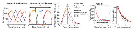
Box 1. Relaxation oscillations of the repressilator.

Depending on parameters, simple repressilators can produce traditional harmonic oscillations with sinusoidal trajectories, as observed in vitro, or relaxation oscillations with separate build-up and relaxation phases (panels below) as we observe experimentally in single cells (middle panel). Due to low abundance fluctuation effects, single cells can in principle also achieve stable oscillations without the traditional requirements of cooperative repression and feedback delays (simulation example in left panel, details in SI). However, having low abundances introduces other constraints. For example, using Poisson communications theory²⁹ we demonstrate (SI §A) hard limits on the ability of such systems to keep track of time, in terms of the average number of molecules N at the peak of the oscillations, even if a repression control system could remember time series of decay events. For circuits like the actual repressilator, where repression is set by the current repressor level, the constraints are more severe yet, and limited both by heterogeneity in N and the inherent noise of the first-order elimination process until levels reach the repression threshold S. Variation in N can be reduced if repressors approach a steady state where production is balanced by elimination (left panel). Noise in N also only has a damped effect on the time to reach a threshold because that time approximately depends logarithmically on N/S: doubling N only adds one more half-life before reaching S. However, substantial noise can arise towards the end of each decay phase if the repression threshold S is too low, as the last few steps then dominate the total decay time (right panel and inset). Specifically, the average length of the decay phase is ${\sum }_{i=S}^{N}1/i\approx log(N/S)$ while the variance is ${\sum }_{i=S}^{N}1/i^2\approx 1/S$ in units of protein half-lives (for details see SI §4.2.2), creating an optimal threshold S_opt that minimizes the CV in the decay time. Increasing N should only significantly reduce this CV if S > S_opt, have virtually no effect if S < S_opt, and decrease the CV in proportion to $\sqrt{N}$ if S is close to S_opt (Extended Data Fig. 4e). Finally, the exponential nature of the decay phase allows the repressilator to be robust to growth conditions: changes in N/S are logarithmically damped in their effects on the average period. Though N and S change with conditions, for many repressors they may change with similar factors that cancel out in the ratio, e.g. because conditions with less gene expression (lowering N) also tend to produce smaller cell volumes (lowering S).

Motivated by these results, we eliminated repressor degradation by removing the ssrA degradation tags from the repressors, by using a ΔclpXP strain, or both (SI §3.3). These circuits indeed oscillated in all cells, with a period of ~10 generations. However, as predicted the noise in the period was only slightly reduced (Fig. 2a, Extended Data Fig. 5c, Extended Data Fig. 6). To pinpoint the reason we built a circuit with compatible fluorescent reporter proteins for each repressor. Analyzing the variance in the three interpeak distances showed that the noisiest phase was when TetR levels were low (Fig. 2b). We then estimated the protein abundances from the partitioning errors at cell division (SI §3.5), and found that the derepression of the TetR controlled promoter occurs at an extremely low threshold.

Figure 2.

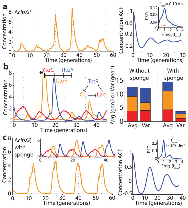
Identifying and eliminating inherent sources of error. a) Typical time trace in ΔclpXP cells (LPT61) where repressors are not degraded. ACF and PSD calculated over 5,356 cell divisions. The average period was 10 generations, and the correlation coefficient was 0.1. Dashed vertical lines are separated by an average period to illustrate periodicity in a–c. b) (Left) Time trace of multi-reporter repressilator (ΔclpXP, LPT113). TetR represses the production of YFP (yellow trace), LacI inhibits the production of CFP (blue trace) and CI represses the production of RFP (red trace). Peak indicated by asterisk not shown due to its high amplitude of 11.5 units. (Right) Interpeak distances evaluated for YFP to CFP (YtoC, red), CFP to RFP (CtoR, yellow) and RFP to YFP (RtoY, blue) without (LPT113, n = 163, 150 and 173) and with the titration sponge (plasmid with P_Ltet binding sites, LPT117 and LPT127, combined, n = 109, 86 and 116). Respective contributions to the average and variance shown by bar plot. The RtoY part of the oscillation (induction of YFP, low TetR levels) represents 27% of the period, but contributes 44% of the variance. Addition of the P_Ltet titration sponge brings down the variance almost fourfold. c) Example time trace of single reporter repressilator with P_Ltet-mCherry-asv (ΔclpXP, LPT64), along with ACF and PSD calculated over 3,695 generations. Oscillations have an average period of 14 generations and a correlation coefficient of 0.5 after one period. Inset shows a time trace from the triple reporter repressilator without degradation and with titration sponge (LPT127, color scheme as in b).

The theory suggests that the regularity could be greatly improved if this threshold was raised, e.g. using a ‘sponge’ of repressor binding sites that soaks up small numbers of TetR molecules. The high-copy reporter plasmid included in the original repressilator design in fact already carried binding sites for TetR, and simply reintroducing it greatly reduced the noise in all steps (Fig. 2b) whereas similar sponges for CI and LacI had minor effects (Extended Data Fig. 7d) as expected. Titration may in fact be a particularly useful way to increase the thresholds because it can also help create sharp switches³⁰ (SI §4.3), which may or may not be necessary for oscillations in single cells but generally should increase accuracy.

These changes created a streamlined repressilator with highly regular oscillations that peak every ~14 generations (Fig. 2c). Each repressor spends several generations at virtually undetectable concentrations (SI §3.5) followed by several generations at concentrations that completely saturate repression. The amplitude still displays some variation (Extended Data Fig. 8d), but because the time it takes to dilute levels from a peak amplitude of N to a threshold of S depends logarithmically on N/S, little variation in amplitude is transmitted to the timing (Box 1, Extended Data Fig. 8e). Indeed the phase drift was only ~14% per period (Extended Data Fig. 5d), i.e., on average the circuit should oscillate for ~18 periods before accumulating half a period of drift (Methods). The theory shows that similar accuracy should be possible in systems where dilution in growing cells is replaced by first order degradation, and that it is not the slowness itself that creates accuracy, but the absolute number of proteins at peaks and troughs.

The periods of circadian clocks, as measured in hours, are often robust to changes in growth conditions. However, other intracellular oscillators may need periods that instead are robust relative to internal physiological time scales such as the generation times. Synthetic circuits generally do not display either type of quantitative robustness because periods depend on so many different parameters that change with conditions. That is in principle also true for the circuits above: as conditions change, plasmid copy numbers, RNA degradation, gene expression, cell volume, etc. change in non-trivial ways. However, the logarithmic dampening that makes individual periods insensitive to fluctuations in peak amplitudes (Box 1) is also predicted to make the number of generations per period insensitive to growth conditions (Box 1). Indeed we found that the circuit retained the 14 generation period under all conditions tested (Fig. 3a), including growth at 25–37°C and in conditioned medium from early stationary phase culture where cells become much smaller and almost spherical. The combination of robustness to conditions and great inherent precision suggest that cells could display macroscopic, population-scale oscillations without cell-cell communication. We therefore synchronized (Extended Data Fig. 9) a liquid culture and maintained it in early exponential phase (Methods). We indeed found that whole flasks oscillated autonomously, with a period of the expected ~14 generations (Fig. 3b, S Video 1). We also imaged the growth of large colonies originating from single cells containing the triple reporter repressilator. Because only the cells at the edges of the colonies grow significantly, cells in the interior were arrested in different repressilator phases, creating ring-like expression profiles much like the seasonal growth rings seen in tree stumps (Fig. 3c, Extended Data Fig. 7a). The regularity originated in the autonomous behavior of single cells – no connections were introduced and cells kept their own phase when merging into areas where the neighboring cells had a different phase (Extended Data Fig. 7c).

Figure 3.

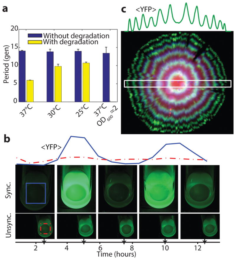
The modified repressilator shows great robustness to growth conditions. a) The repressilator without degradation and with titration sponge (LPT64) has a period of 14 generations at different temperatures (blue bars, division time of 27, 40 and 59 min for 37°C, 30°C and 25°C respectively) and in conditioned media (OD₆₀₀ ~2, doubling time of 44 min). Repressilator with repressor degradation (LPT25) shows a varying period (yellow bars, doubling time of 26, 34 and 52 min for 37°C, 30°C and 25°C respectively). Error bars indicate STD on the first maximum of the ACF obtained by bootstrapping. b) Cells containing multi-reporter repressilator without repressor degradation and with P_Ltet-peptide-asv plasmid (ΔclpXP, LPT117) were grown in liquid culture in 25mL flasks. After the culture was initially synchronized with IPTG, it was kept in exponential phase via dilution. Average YFP intensity shown for colored square area, with unsychronized culture for comparison. c) A ~5 mm diameter colony of cells with the triple reporter repressilator (LPT117) reveals tree-like ring patterns in FP levels. The average YFP intensity is reported for the slice in the white rectangle. The decrease in RFP levels towards the edge of the colony is likely due to different response to stationary phase of its promoter.

The results above (summarized in Extended Data Fig. 10) illustrate the importance of understanding genetic networks at the level of stochastic chemistry, particularly for synthetic circuits where the noise has not been shaped by natural selection and where the heterologous components and reporters used may interfere with cells. We hypothesize that if statistical properties are systematically measured and the mechanisms are iteratively redesigned based on general stochastic principles, the next generation of synthetic circuits could rival or even surpass the precision of natural systems.

METHODS

Data and materials availability

Segmented and assembled single-cell traces files are accessible online. The masks files used for the microfluidic device master fabrication are available on request. The plasmids have been deposited to the Addgene plasmid repository, and the plasmids maps are available online.

Imaging protocol

Chip preparation

Dimethyl siloxane monomer (Sylgard 184) was mixed in a 10:1 ratio with curing agent, defoamed, poured onto the silicon wafer, degassed for 1 hour and cured at 65°C for 1 hour. Individual chips were then cut and the inlets and outlets were punched with a biopsy puncher. Bonding to KOH-cleaned cover slips was ensured using oxygen plasma treatment (30 sec at 50 W and O₂ pressure at 170 mTorr) on the day the experiments start. The chips were then incubated at 95°C for at least 30 min to reinforce the bonding.

Cell preparation

E. coli strains were grown overnight in LB with appropriate antibiotics and diluted 1:100 ~2–3 hours before the beginning of the experiments in imaging media, consisting of M9 salts, 10% (v/v) LB, 0.2% (w/v) glucose, 2 mM MgSO₄, 0.1 mM CaCl₂, 1.5 μM thiamine hydrochloride and 0.85 g/L Pluronic F-108 (Sigma Aldrich, included as a passivating agent). The cells were loaded into the device at OD₆₀₀ 0.2–0.4, and centrifuged on a custom-machined holder that could fit into a standard table-top centrifuge at 5000 g for 10 min to insert them into the side-channels. The feeding channels were connected to syringes filled with imaging media using Tygon tubing (VWR), and media was pumped using syringe pumps (New Era Pump System) initially at a high rate of 100 μL/min for 1 hour, to clear the inlets and outlets. The media was then pumped at 5–10 μL/min for the duration of the experiment and cells were allowed to adapt to the device for multiple hours before imaging was started.

Microscopy and image acquisition

Images were acquired using a Nikon Ti inverted microscope equipped with a temperature-controlled incubator, an Orca R2 CCD camera (Hamamatsu), a 60X Plan Apo oil objective (NA 1.4, Nikon), an automated xy-stage (Ludl) and light engine LED excitation source (Lumencor). All experiments were performed at 37°C. Microscope control was done with MATLAB (Mathworks) scripts interfacing with μManager³¹. Typical exposure was low (50–100 ms) in order to reduce photobleaching, and the reporter channels were acquired using 2×2 binning (CCD chip dimension of 1344 × 1024 pixels, effective pixel size of 129nm × 129nm). 16 bits TIFF images were taken every 5–8 minutes, and focal drift was controlled via the Nikon PerfectFocus system, as well as a custom routine based on z-stack images of a sacrificial position. The following filter sets were used for acquisition: GFP (Semrock GFP-3035B), RFP (Semrock mCherry-A), YFP (Semrock YFP-2427A) and CFP (Semrock CFP-2432A).

Conditioned medium

The conditioned medium was obtained by growing the strain used in the experiment until OD₆₀₀ = 2.0, and then the culture was rapidly sterilized with a 0.2μm filter and kept at 4°C until the experiment.

IPTG

When indicated, the imaging medium was supplemented with isopropyl β-D-1-thiogalactopyranoside (IPTG) for the duration indicated in the figure.

Data processing

Segmentation

Image segmentation and single-cell trace assembly were performed similarly to a previously described procedure²³. Briefly, the segmentation was done using images from a bright, constituvely expressed (P_RNA1 promoter on the chromosome or on the plasmid) CFP or RFP. The rough channel boundaries were estimated, in order to reject out-of-channel cells, with a simple threshold followed by erosion, opening and dilation of the mask. The contrast of the fluorescent image was enhanced using a ‘unsharp mask’. Then, the edges of the cells were detected using the Laplacian of Gaussian method. Cells joined by their poles (as indicated by objects with definite constrictions) were separated, and spurious non-cell objects were rejected using their size, orientation and shape. Finally, the boundaries were refined using opening, thickening and active contours. The parameters used for these functions were optimized specifically for the combination of the strain, growth conditions and microscope setup. We will share the code used on request, but the specific parameters will need to be re-optimized depending on the exact setup.

We chose to follow only the cells at the top (closed end) of the channel (the ‘mother’ cell), as it made compiling the single-cell traces much easier as these cells stay in place for the duration of the experiment. Due to physical limitations of the setup, the segmentation mask was slightly mis-registered with respect to the ‘data channel’ (i.e. GFP or YFP). Each object was then registered to the proper channel before the data were extracted.

For the triple reporter strains (that did not contain a specific segmentation fluorophore), we combined the three reporters channels according to their signal-to-noise ratio to obtain an effective segmentation channel. In some cases, we used an alternative procedure where the whole channels were segmented, and the top 50 pixels were used as a ‘cell’ which represented one to two cells. Because the oscillations for these analyses were very slow and the cells in the channels are very close in phase (e.g. see Extended Data Fig. 5g), the two methods gave very similar results to the normal procedure, but in general the ‘channel’ analysis worked more reliably. This analysis was only used in Fig. 2b.

The background fluorescence was corrected by subtracting the median value of the fluorescent images (the cells represent a very small fraction of the image). We then estimated the concentration of fluorophore using the average of the background-substracted intensities inside the segmentation mask. Nearly identical results were obtained using the ‘peak’ intensity (median of the top 10 % of the pixel in the segmentation mask), but for simplicity we only report the results obtained with the mean.

Single-cell traces construction

The temporal information of the cell data (intensities, area, etc.) was then compiled into single-cell traces by matching the centroid of the cells from frame n to frame n+1. As there was little drift, this procedure was very reliable, and we prevented spurious matches by setting an upper limit on the centroid distance. We identified cell divisions by sudden decreases in cell area; if the cell area dropped to less than 60% of its previous value, a division was called.

Production rate estimation

To estimate the production rate of fluorophore, we used the derivative of the concentration, as it was more robust to errors in segmentation. Let T be the total intensity, A the area of the cell and C the concentration. Since T(t) = A(t)C(t),

$$\begin{gathered} \frac{dT}{dt}=C\frac{dA}{dt}+A\frac{dC}{dt} \\ \frac{1}{A}\frac{dT}{dt}=C\frac{1}{A}\frac{dA}{dt}+\frac{dC}{dt} \\ P(t)=C(t)g(t)+\frac{dC}{dt} \end{gathered}$$ (1)

where $P(t)=\frac{1}{A}\frac{dT}{dt}$ is the normalized production rate and g(t) is the growth rate (e.g. g = ln(2)/τ_div for exponential growth, A(t) = A₀2^t/τ_div, τ_div being the doubling time). Equation 1 was used for estimating the production rate in the paper, with g(t) estimated for each cell cycle with the initial and final area and dC/dt using Tikhonov regularization to enforce smoothness³². The normalization factor was kept as small as possible, but similar results were obtained for factors one order of magnitude smaller or larger. In practice, photobleaching or degradation of the fluorescent protein can affect the estimation of the production rate. One can account for these effects by using an effective half-life instead of τ_div (e.g. ${\tau }_{\mathit{eff}}^{-1}={\tau }_{\mathit{div}}^{-1}+{\tau }_{\mathit{photo}}^{-1}+{\tau }_{\mathit{deg}}^{-1}$, where τ_photo and τ_deg are the photobleaching and degradation half-lives, respectively). These effects were negligible for GFP (even with the asv degradation tags), so we chose to report the production rate without correction.

Autocorrelation function and power spectrum estimation

The autocorrelation functions were estimated by averaging the correlation functions of the individual cells, as it was more robust to outliers, and using the unbiased estimator. Similar functions were obtained by taking directly the autocorrelation of the population, but needed manual curation of the data to remove dead cells or filaments.

$$A(\tau )={\langle \frac{{\langle (x_i(t)-{\langle x_i(t)\rangle }_t)(x_i(t+\tau )-{\langle x_i(t)\rangle }_t)\rangle }_t}{{\langle x_i{(t)}^2\rangle }_t}\rangle }_i$$ (2)

where x_i(t) is the production rate or the concentration (indicated in the figure caption) of the i^th cell at time t. Averaging of the correlations functions of the cells was done taking into account the finite length of the time series (each cell has a different number of samples for a specific time lag). If A_i is the autocorrelation of cell i,

$$\widehat{A}[j]=\frac{{\sum }_i(L_i-j){\widehat{A}}_i[j]}{{\sum }_i(L_i-j)}$$ (3)

with A(jΔt) = Â[j], Δt the time between images, j the discrete delay index and L_i the number of points in time trace i. The brackets are used to emphasize discrete sampling. The autocorrelations were cropped to a constantly decreasing envelope to keep only time lags with good estimates. This resulted in correlation functions very similar to the ones obtained by using the biased estimator, albeit with a slightly larger envelope.

The power spectrum was then estimated by taking the discrete Fourier transform (DFT) of the windowed autocorrelation function^{33, 34}:

$$P[k]={\text{DFT}}_N(a[m])$$ (4)

where DFT_N is the N point DFT and a[m] is the windowed symmetric autocorrelation:

$$a[m]=\{\begin{array}{ll}\widehat{A}[\mid M-m\mid ]w[m]\hfill & \text{for}0\le m\le 2M\hfill \\ 0\hfill & \text{for}2M<m\le N\hfill \end{array}$$ (5)

and w[m] is a window function. Then,

$$P[k]=P{(w)\mid }_{\omega =2\pi k/N}$$ (6)

$$P(\omega )=\frac{1}{2\pi }{\int }_{-\pi }^{\pi }X(\theta )W(\omega -\theta )d\theta$$ (7)

where X(ω) is the power spectrum of the signal and W(ω) the Fourier transform of the window function. We are therefore sampling the power spectrum of the signal convolved with W(ω). This is a consistent estimator of the power spectrum (it converges to the actual power spectrum as the amount of data goes to infinity)³⁵. We used a triangular window function to avoid negative spectral leakage, and the length of the window function (2M) was chosen to maximize the resolution without introducing too much noise (50–225 frames, depending on the period of the oscillations). The approximate resolution loss was indicated by a red line of width 2π/M (1/(MΔt)) in the figures.

Period histograms and phase drift estimation

Peak-to-peak distances were evaluated by finding maxima using the findpeaks MATLAB function. The traces were first smoothed using a 3 or 5 points moving average and peaks were rejected if they were closer than 3 or 5 frames to avoid double counting, or smaller than the average of the trace. The peaks were then manually curated; this was especially useful for the noisy oscillators. Note that the average period was slighly shorter than the first maximum of the autocorrelation, most likely because longer periods have higher intensities and thus more weights in the correlation (but not in the period histogram).

The period histograms were made by using the peak-to-peak distance. The squared error on the n^th period grew linearly with n, as expected for this type of oscillator undergoing a random walk in phase. We therefore used the coefficient of variation (CV, standard deviation divided by the mean) of the period as an indicator of phase drift; the normalization makes comparison between oscillators of different frequencies straightforward.

Most of the strains had a phase drift of 30–35% per period; except for the repressilator without degradation but with the titration sponge, where it was only 14%. Since the variance increased linearly, we can express the variance for n periods ( ${\sigma }_n^2$) as a function of the variance for one ( ${\sigma }_1^2$):

$$\begin{gathered} {\sigma }_n^2=n{\sigma }_1^2 \\ {\sigma }_n={\sigma }_1\sqrt{n} \\ =\langle \text{period}\rangle \times \text{CV}\sqrt{n} \end{gathered}$$

Hence, it would take ~13 periods (~179 generations) to obtain a standard deviation of half a period.

Another measure of the phase drift is the average time to reach half a period of phase drift, or the average first passage time. This could be calculated by drawing randomly directly from the period histogram until the first time the phase drift is reached, because subsequent periods were exceptionally well approximated as independent (Fig. 1f). This creates a distribution of first passage times, and after 10⁵ iterations, we converge on an average first passage time of ~ 18 periods (~ 240 generations), again for the repressilator without degradation with titration (LPT64).

Macroscopic image acquisition

IPTG synchronization and flask experiment

In order to synchronize the phase of the oscillators in the population, we diluted the strains in imaging medium supplemented with appropriate antibiotics and 1 mM IPTG so that they would be early exponential (OD₆₀₀ ~ 0.2) 8 hours later (~ 1 : 10⁶) at 37°C. For the unsynchronized control, we did the same procedure but did not include IPTG. After, we diluted the cultures to OD₆₀₀ 0.05 every 50 min, while taking the fluorescent images of the (undiluted) flasks. The OD₆₀₀ of the imaged culture varied slightly, but the effect was negligible, as can be seen on the unsynchronized control (Fig. 3b).

Photo acquisition

Photos were acquired using a digital camera setup equipped with emission filters and LEDs fluorescent excitation³⁶. A custom written software controls a Canon T3i digital single lens reflex (DSLR) camera with a Canon EF-S 60mm USM lens, placed in front of a Starlight express filter wheel, and appropriate LEDs for excitation. A long exposition time of 10 s was used for the flask – enabling the use of small OD₆₀₀ – while the exposition time of the plates was 0.1–2 s.

Microscopy

Images for figure 3c were acquired using a Olympus MVX10 Macroview microscope equipped with a Zeiss AxioCam MRc camera. Flurophores were excited using a Lumen200 fluorescence illumination system (Prior Scientific) and we used the following Olympus filter sets: CFP (U-M40001XL), YFP (U-M49003XL) and mCherry (U-M49008XL).

Extended Data

Extended Data Figure 1.

Oscillations in the original and integrated repressilator circuits. a) Original (NDL332, GFP production rate) and b) integrated repressilator (LPT25, YFP concentration) oscillations are sustained for more than one hundred generations. The two time traces were normalized to their respective means. Three peaks in a) indicated by asterisks have been clipped due to their high amplitude (5.9, 7.1 and 4.8) to allow better visualization of the oscillations. IPTG was added to the media for the time period indicated by the red bar (in a) in order to synchronize the cells in the device.

Extended Data Figure 2.

Interference from the reporter plasmid. a) Oscillations of the integrated repressilator with the P_Ltet-mCherry-asv plasmid (LPT54) have a more constant peak amplitude compared to the original repressilator, indicated by the CV of the peak amplitude decreasing from 0.78 to 0.36 (b). The inset in b) zooms in on the tails of the distributions. c) Additional plasmid loss event of integrated repressilator with P_Ltet-mCherry-asv reporter. The reporter plasmid is lost around generation 34, as evidenced by the loss of red fluorescence. The oscillation period shifts from ~2 to ~5 generations quickly after the plasmid loss event. d) Example time trace of the integrated repressilator, without the reporter plasmid (LPT25). The YFP production rate oscillates (yellow trace), while the segmentation marker (blue trace) stays relatively constant (close-up of the shaded region on top). Both traces were normalized to their respective means. e) Autocorrelation function (ACF) and power spectral density (PSD) were calculated over the whole population (8,694 total generations) and demonstrate strong oscillatory behavior, with an average period of 5.6 generations. The width of the window function used for calculating the power spectrum is indicated by a red line.

Extended Data Figure 3.

Summary of results explaining the difference in period between the original and integrated repressilator. a) The P_Ltet sponge (LPT44) makes the oscillation slightly shorter and more regular compared to the empty plasmid (LPT45), but cannot explain the change in period. b) Increasing the expression of ‘competing’ substrates tagged with the asv tag makes the oscillations faster. The period gradually decreases from 5.5 generations for the empty plasmid (LPT45) to 4.2 with P_Ltet-pep-asv (LPT46), to 2.6 with P_Ltet-mCherry-asv (LPT54) and to 2.3 with P_const-darkGFP-asv (LPT53). c) Removing the degradation tag on the reporter of the original repressilator (LPT60) produces oscillations very similar to the integrated repressilator with the sponge (LPT44). d) Summary of the period of the different construct presented in this figure, compared to the original (NDL332) and integrated repressilator (LPT25). Introduction of ASV-tagged molecules is sufficient to explain the change in period, whereas introduction of LAA-tagged molecules slows down the oscillations (LPT55). Overexpressing a functional ClpP-mGFPmut3 fusion makes the period slightly faster (5.4 gen, LPT159), but does not rescue the effect of the ASV-tagged proteins (2.8 gen, LPT165). e) Expressing ASV-tagged molecules in the absence of the repressilator lowers the mean abundances of ssrA-tagged molecules ~ four-fold, suggesting that presence of ASV-tagged molecules cause faster degradation rates. f) In the ΔclpXP background, the oscillations are not affected by the presence of ASV-tagged molecules or additional reporter. Triple reporter with P_Ltet sponge (LPT127), triple with P_Ltet-mCherry-asv (LPT118) and single with P_Ltet-mCherry-asv (LPT64) have very similar autocorrelation functions and ring patterns (g-h-i). There were slight variations in the imaging conditions due to manual focusing and non-uniformity of the LED illumination.

Extended Data Figure 4.

Modeling results. a) The repressilator can display harmonic or relaxation oscillations. The gradual transition between the regimes is shown here by varying the parameter K in the minimal model (λ = 2000 and n = 4, SI §4.1). b) The experimental data suggest that the repressilator oscillates in the relaxation regime. Simulated time trace (blue, K = 13, λ = 10³, and n = 3 ) is overlayed with time trace of experimental data (from Fig. 2c, LPT64, yellow). c) Close-up of a simulated time trace (minimal model, K = 0.2, λ = 10³, and n = 2, SI §4.1) in the relaxation regime showing the three different repressors (blue, red and yellow). The oscillations can be separated in two distinct phases: an accumulation phase during which the protein (blue) is completely derepressed (red below threshold) and starts at very low numbers, and a decay phase that starts when the repressor is completely repressed (red above threshold) and ends when it goes below the repression threshold of the next component (yellow starts to accumulate). d) Relaxation oscillators have different parameter requirements for oscillations. Simulated time traces (solid lines) show oscillations without biochemical cooperativity or phase shift due to the presence of mRNA (minimal model, K = 0.01, λ = 10³, and n = 1, SI §4.1). The deterministic differential equations with the same parameters show damped oscillations (dashed lines with flipped colors). e) Even for perfect threshold mechanism, significant noise comes from the decay phase if the threshold (S) is too low (or too high) with respect to the peak value (N). If S ≪ N, then the CV in one decay step goes down very slowly (1/log(N/(S + 1))). However, if it is reasonably close to its optimal value (e.g. 0.05 < S/N < 0.3), it goes down much faster ( $1/\sqrt{N}$). The CV is shown for different combination of S and N, as well as the asymptotic traces. f) Simulated time trace of the model of SI §4.3.1 shows oscillations of similar shape, peak amplitude numbers, period and phase drift as the experimental data by using reasonable parameters (λ = 60, K = (5, 10, 10) for the three repressors, n = 1.5 for all repressors, 〈b〉 = 10, 〈N_o〉 = 10 〈N_t〉 = 40).

Extended Data Figure 5.

Period histograms and kymographs of selected strains. Peak-to-peak distance of the oscillations was calculated as described in Methods, and the average period, as well as the CV (standard deviation divided by the mean) are reported in the figure panels. a) Original repressilator (NDL332). b) Integrated repressilator (LPT25). c) Integrated repressilator in ΔclpXP (LPT61). d) Integrated repressilator in ΔclpXP with P_Ltet-mCherry-asv (LPT64). e) Integrated repressilator with P_Ltet sponge (LPT44). f) Integrated repressilator with P_Ltet-mCherry-asv (LPT54) g) Kymograph (xy-t montage) of the raw data is presented for three strains. The image of a single growth channel is presented every 1, 2 and 7 frames (5 min/frame) for the top, middle and bottom panel respectively. The oscillations in concentration are difficult to see in the fast oscillator (although clear when looking at production rate), but they can be clearly seen in the slow oscillators. The growth channels are open towards the bottom of the images, where media is supplied.

Extended Data Figure 6.

Oscillations of the repressilator without degradation tags. a) Schematic of integrated repressilator without degradation tags, with or without the P_Ltet titration sponge. b) Without the titration sponge (LPT120), the oscillations are erratic in amplitude, with a correlation coefficient of ~0.1 after one period. c) Addition of the sponge (LPT124) makes the oscillations much more regular, with a correlation coefficient of ~0.25 after one period. d) Time trace and autocorrelation of integrated repressilator without degradation tags in ΔclpXP (LPT128). Introduction of the mutation did not change the oscillations substantially (compared to c). e) The colonies of integrated repressilator without degradation tags with P_Ltet sponge (LPT124) exhibit spatio-temporal ring patterns in the YFP images. f) Close-up of the colonies show that the spatio-temporal patterns were similar if the titration sponge contained only the promoter (LPT124) or expressed an ASV-tagged peptide (LPT125), suggesting that these strains have similar oscillations.

Extended Data Figure 7.

Macroscopic spatial patterns of the repressilator. a) Time course growth of a single colony grown from a ΔclpXP mutant cell containing the integrated repressilator and titration sponge (LPT64, P_Ltet-mCherry-asv). Oscillations in YFP levels produce macroscopic, ringed structures in the YFP channel (bottom row), while such patterns are absent in the constitutive segmentation marker (CFP, middle row) and gross colony morphology (bright field, top row). The bottom and left white spots in the brightfield images are reflections from the white LEDs. b) On the left, unsynchronized cells were plated and different phases of the oscillators are represented by different ring patterns (dark or bright center of different sizes). Synchronization of the cells with IPTG makes the patterns similar, with a dark center of the same size. c) The ring patterns do not synchronize when adjacent colonies merge into each other. d) Only the presence of the P_Ltet sponge is required for macroscopic oscillations, while titration of the other repressors do not affect greatly the oscillations. From left to right: LPT153, LPT154, LPT157, LPT143, LPT155, LPT156 and LPT152. Several strains were also evaluated in the microfluidic device.

Extended Data Figure 8.

Characterization of the microfluidic device and of the oscillations. a) The average division time of the integrated repressilator (LPT25) is constant over time. The inset shows the distribution of growth rates of two independent experiments (45,828 and 9,135 points are shown in the blue and red distributions, respectively), with a slight difference in the mean (~ 1%). b) The period of the oscillations is constant in space (position in field of view, distance to inlets and outlets and different media channels) and time. Each point represents a bin of 400 (a) or 100 (b) points, with the error bars indicating standard error of the mean. c) The induction/repression switch of CI (reported by YFP) occurs when the transcriptional reporter for TetR (CFP) is below the detection limit. Typical time trace of multireporter repressilator without repressor degradation and with P_Ltet-peptide-asv plasmid (ΔclpXP, LPT117). The production rate of YFP is shown alongside the CFP concentration. The inset shows that the switch from induction to repression occurs below the detection limit of ~ 50 FU. d) The distribution of peak amplitude of the repressilator without degradation but with titration sponge shows significant heterogeneity (LPT64, CV of 35%). e) The peak amplitude has a small influence on the next period, due to exponential dilution. The red line shows a fit to y = 1.99 * log(x)+13.18 and explains 25% of the variance in the periods. Black circles are bins of 15 points of black dots (LPT64) and blue dots (LPT156). f) Estimating partitioning root mean squared (RMS) errors at cell division during the dilution phase showed that it scaled binomially, and allowed us to roughly estimate a fluorescence units to protein scaling factor. Black circles are bins of 50 blue dots (LPT64). The red line shows the fit (after conversion) to $\sqrt{\langle {(n_1-n_2)}^2\rangle }=\sqrt{N}$, where n_i is the number of proteins in the daughters right after division, and N = n₁ + n₂ the number in the mother cell. g) Typical time trace of triple reporter repressilator without degradation with titration sponge (LPT127) in estimated protein numbers (concentration × average cell size).

Extended Data Figure 9.

Robustness and synchronization of the oscillations. a) The phase of the oscillations is independent of the phase of the cell cycle. The average phase of the oscillation phase is shown as a function of the position in the cell cycle. Each point represents a bin of 3,000 data points, which have been average in x and y after being sorted on their x values. The error bars represent standard error on the mean and are of similar size to the symbols. Similar results were obtained for different strains, but here are shown for the integrated repressilator (LPT25). b) Synchronization of different cells in the microfluidic device was done by introducing 1mM IPTG. The original repressilator (NDL332) shows a modest level of synchrony in the oscillations of the GFP production rate. c) The integrated repressilator shows a more robust synchronization in the YFP production rates, but takes more time to recover from the pertubation.

Extended Data Figure 10.

Schematic of the major changes to the repressilator and resulting effects on the oscillations. The original repressilator displays sustained oscillation with a period of 2.4 generations, albeit with a variable amplitude. Integrating the reporter on the pSC101 plasmid decreases the peak amplitude CV from 78% to 36%. Then, removing the presence of ASV-tagged molecules increases the period to 5.7 generations, due to the interference with degradation of the repressors in the former case. Removing degradation entirely increases the period to 10 generations, but significant amplitude and phase drift subsist. Reintroducing a sponge of binding site for the TetR repressors raises the repression threshold and enables the repressilator to exhibit precise oscillations (as well as macroscopic oscillations), by decreasing the period CV from 28% to 14% and increasing the period to 14 generations. Typical time traces are shown from top to bottom of NDL332, LPT54, LPT25, LPT61 and LPT127.

References

- 1.Elowitz MB, Leibler S. A synthetic oscillatory network of transcriptional regulators. Nature. 2000;403:335–338. doi: 10.1038/35002125. [DOI] [PubMed] [Google Scholar]
- 2.Nakajima M, et al. Reconstitution of Circadian Oscillation of Cyanobacterial KaiC Phosphorylation in Vitro. Science. 2005;308:414–415. doi: 10.1126/science.1108451. [DOI] [PubMed] [Google Scholar]
- 3.Teng SW, Mukherji S, Moffitt JR, de Buyl S, O’Shea EK. Robust circadian oscillations in growing cyanobacteria require transcriptional feedback. Science. 2013;340:737–40. doi: 10.1126/science.1230996. [DOI] [PMC free article] [PubMed] [Google Scholar]
- 4.Mihalcescu I, Hsing W, Leibler S. Resilient circadian oscillator revealed in individual cyanobacteria. Nature. 2004;430:81–85. doi: 10.1038/nature02533. [DOI] [PubMed] [Google Scholar]
- 5.Chabot JR, Pedraza JM, Luitel P, van Oudenaarden A. Stochastic gene expression out-of-steady-state in the cyanobacterial circadian clock. Nature. 2007;450:1249–1252. doi: 10.1038/nature06395. [DOI] [PubMed] [Google Scholar]
- 6.Friedland AE, et al. Synthetic gene networks that count. Science. 2009;324:1199–202. doi: 10.1126/science.1172005. [DOI] [PMC free article] [PubMed] [Google Scholar]
- 7.Daniel R, Rubens JR, Sarpeshkar R, Lu TK. Synthetic analog computation in living cells. Nature. 2013 doi: 10.1038/nature12148. [DOI] [PubMed] [Google Scholar]
- 8.Fung E, et al. A synthetic gene-metabolic oscillator. Nature. 2005;435:118–122. doi: 10.1038/nature03508. [DOI] [PubMed] [Google Scholar]
- 9.Stricker J, et al. A fast, robust and tunable synthetic gene oscillator. Nature. 2008;456:516–519. doi: 10.1038/nature07389. [DOI] [PMC free article] [PubMed] [Google Scholar]
- 10.Tigges M, Marquez-Lago TT, Stelling J, Fussenegger M. A tunable synthetic mammalian oscillator. Nature. 2009;457:309–312. doi: 10.1038/nature07616. [DOI] [PubMed] [Google Scholar]
- 11.Danino T, Mondragón-Palomino O, Tsimring L, Hasty J. A synchronized quorum of genetic clocks. Nature. 2010;463:326–30. doi: 10.1038/nature08753. [DOI] [PMC free article] [PubMed] [Google Scholar]
- 12.Mondragón-Palomino O, Danino T, Selimkhanov J, Tsimring L, Hasty J. Entrainment of a population of synthetic genetic oscillators. Science. 2011;333:1315–9. doi: 10.1126/science.1205369. [DOI] [PMC free article] [PubMed] [Google Scholar]
- 13.Prindle A, et al. Rapid and tunable post-translational coupling of genetic circuits. Nature. 2014 doi: 10.1038/nature13238. [DOI] [PMC free article] [PubMed] [Google Scholar]
- 14.Bonnet J, Yin P, Ortiz ME, Subsoontorn P, Endy D. Amplifying Genetic Logic Gates. Science. 2013 doi: 10.1126/science.1232758. [DOI] [PubMed] [Google Scholar]
- 15.Tabor JJ, et al. A synthetic genetic edge detection program. Cell. 2009;137:1272–81. doi: 10.1016/j.cell.2009.04.048. [DOI] [PMC free article] [PubMed] [Google Scholar]
- 16.Paulsson J, Berg OG, Ehrenberg M. Stochastic focusing: fluctuation-enhanced sensitivity of intracellular regulation. Proc Natl Acad Sci USA. 2000;97:7148–7153. doi: 10.1073/pnas.110057697. [DOI] [PMC free article] [PubMed] [Google Scholar]
- 17.Vilar JMG, Kueh HY, Barkai N, Leibler S. Mechanisms of noise-resistance in genetic oscillators. Proc Natl Acad Sci USA. 2002;99:5988–92. doi: 10.1073/pnas.092133899. [DOI] [PMC free article] [PubMed] [Google Scholar]
- 18.McKane aJ, Newman TJ. Predator-Prey Cycles from Resonant Amplification of Demographic Stochasticity. Physical Review Letters. 2005;94:218102. doi: 10.1103/PhysRevLett.94.218102. [DOI] [PubMed] [Google Scholar]
- 19.Lestas I, Vinnicombe G, Paulsson J. Fundamental limits on the suppression of molecular fluctuations. Nature. 2010;467:174–178. doi: 10.1038/nature09333. [DOI] [PMC free article] [PubMed] [Google Scholar]
- 20.Keiler K, Waller P, Sauer R. Role of a peptide tagging system in degradation of proteins synthesized from damaged messenger RNA. Science. 1996;271:990–993. doi: 10.1126/science.271.5251.990. [DOI] [PubMed] [Google Scholar]
- 21.Andersen JB, et al. New unstable variants of green fluorescent protein for studies of transient gene expression in bacteria. Appl Environ Microbiol. 1998;64:2240–2246. doi: 10.1128/aem.64.6.2240-2246.1998. [DOI] [PMC free article] [PubMed] [Google Scholar]
- 22.Wang P, et al. Robust growth of Escherichia coli. Curr Biol. 2010;20:1099–1103. doi: 10.1016/j.cub.2010.04.045. [DOI] [PMC free article] [PubMed] [Google Scholar]
- 23.Norman TM, Lord ND, Paulsson J, Losick R. Memory and modularity in cell-fate decision making. Nature. 2013;503:481–6. doi: 10.1038/nature12804. [DOI] [PMC free article] [PubMed] [Google Scholar]
- 24.Paulsson J, Ehrenberg M. Noise in a minimal regulatory network: plasmid copy number control. Q Rev Biophys. 2001;34:1–59. doi: 10.1017/s0033583501003663. [DOI] [PubMed] [Google Scholar]
- 25.Moriya T, Yamamura M, Kiga D. Effects of downstream genes on synthetic genetic circuits. BMC Systems Biology. 2014;8:S4. doi: 10.1186/1752-0509-8-S4-S4. [DOI] [PMC free article] [PubMed] [Google Scholar]
- 26.Berg OG, Paulsson J, Ehrenberg M. Fluctuations and quality of control in biological cells: zero-order ultrasensitivity reinvestigated. Biophysical journal. 2000;79:1228–1236. doi: 10.1016/S0006-3495(00)76377-6. [DOI] [PMC free article] [PubMed] [Google Scholar]
- 27.Niederholtmeyer H, et al. Rapid cell-free forward engineering of novel genetic ring oscillators. eLife. 2015:e09771. doi: 10.7554/eLife.09771. [DOI] [PMC free article] [PubMed] [Google Scholar]
- 28.van der Pol B. On relaxation-oscillations. Philosophical Magazine. 1926;2:978–992. [Google Scholar]
- 29.Verdú S. Poisson communication theory. Invited talk. 1999 Mar;25 [Google Scholar]
- 30.Brewster R, et al. The Transcription Factor Titration Effect Dictates Level of Gene Expression. Cell. 2014;156:1312–1323. doi: 10.1016/j.cell.2014.02.022. [DOI] [PMC free article] [PubMed] [Google Scholar]
- 31.Edelstein A, Amodaj N, Hoover K, Vale R, Stuurman N. Computer control of microscopes using microManager. Current protocols in molecular biology. 2010;Chapter 14(Unit14.20) doi: 10.1002/0471142727.mb1420s92. [DOI] [PMC free article] [PubMed] [Google Scholar]
- 32.Tikhonov AN, Arsenin VY. Solutions of Ill-Posed Problems. Mathematics of Computation. 1978;32:1320–2. [Google Scholar]
- 33.Blackman RB, Tukey JW. The measurement of power spectra. Dover Publications; New York, NY: 1958. [Google Scholar]
- 34.Oppenheim AV, Schafer RW. Discrete-time signal processing. 3 Prentice Hall; Upper Saddle River, NJ: 1989. [Google Scholar]
- 35.Jenkins GM, Watts DG. Spectral Analysis. 1968 [Google Scholar]
- 36.Chait R, Shrestha S, Shah AK, Michel JB, Kishony R. A differential drug screen for compounds that select against antibiotic resistance. PloS one. 2010;5:e15179. doi: 10.1371/journal.pone.0015179. [DOI] [PMC free article] [PubMed] [Google Scholar]
Associated Data
This section collects any data citations, data availability statements, or supplementary materials included in this article.