EigenPrism: inference for high dimensional signal-to-noise ratios

Abstract

Consider the following three important problems in statistical inference, namely, constructing confidence intervals for (1) the error of a high-dimensional (p > n) regression estimator, (2) the linear regression noise level, and (3) the genetic signal-to-noise ratio of a continuous-valued trait (related to the heritability). All three problems turn out to be closely related to the little-studied problem of performing inference on the ${\ell }_2$-norm of the signal in high-dimensional linear regression. We derive a novel procedure for this, which is asymptotically correct when the covariates are multivariate Gaussian and produces valid confidence intervals in finite samples as well. The procedure, called EigenPrism, is computationally fast and makes no assumptions on coefficient sparsity or knowledge of the noise level. We investigate the width of the EigenPrism confidence intervals, including a comparison with a Bayesian setting in which our interval is just 5% wider than the Bayes credible interval. We are then able to unify the three aforementioned problems by showing that the EigenPrism procedure with only minor modifications is able to make important contributions to all three. We also investigate the robustness of coverage and find that the method applies in practice and in finite samples much more widely than just the case of multivariate Gaussian covariates. Finally, we apply EigenPrism to a genetic dataset to estimate the genetic signal-to-noise ratio for a number of continuous phenotypes.

1 Introduction

1.1 Problem Statement

Throughout this paper we will assume the linear model

$$\mathit{y}=\mathit{X}\beta +\epsilon ,$$ (1.1)

where y, $\epsilon \in {\mathbb{R}}^n$, $\beta \in {\mathbb{R}}^p$, and $\mathit{X}\in {\mathbb{R}}^{n\times p}$. Denote the i^th row and j^th column of X by x_i and X_j, respectively. We assume the x_i are drawn i.i.d. from a mean-zero distribution with covariance matrix Σ.

Our goal is to construct a two-sided confidence interval (CI) for the expected signal squared magnitude ${{\Sigma }^{1∕2}\beta \Vert }_2^2$ (or equivalently just θ). Explicitly, for a given significance level α ∈ (0, 1), we want to produce statistics L_α and U_α, computed from the data, obeying

$$\begin{array}{cc}\hfill \mathbb{P}({\theta }^2<L_{\alpha })& \le \alpha ∕2,\hfill \\ \hfill \mathbb{P}({\theta }^2>U_{\alpha })& \le \alpha ∕2.\hfill \end{array}$$ (1.2)

In words, we want to be able to make the following statement: “with 100(1 – α)% confidence, θ² lies between L_α and U_α.”

1.2 Motivation

This problem can be motivated first from a high level as an approach to performing inference on β in high dimensions. Since p > n, we cannot hope to perform inference on the individual elements of β directly (without further assumptions, such as sparsity), but there is hope for the one-dimensional parameter θ. Although θ is not often considered a parameter of inference in regression problems, it turns out to be closely related to a number of well-studied problems.

Suppose one has an estimator $\widehat{\beta }$ for β. Perhaps the most important question to be asked is: how close is $\widehat{\beta }$ to β? This question can be answered statistically by estimating and/or constructing a CI for the error of that estimate, namely, ${\Vert \widehat{\beta }-\beta \Vert }_2$. This is a fundamental statistical problem arising in many applications. Consider, for example, a compressed sensing (CS) experiment in which a doctor performs an MRI on a patient. In MRI, the image is observed not in the spatial domain, but in the frequency domain. If as many observations as pixels are made, the result is the Fourier transform (with some added noise) of the image, from which the original spatial pixels can be inferred. CS theory suggests that one can instead use a number of observations (rows of the Fourier matrix) that is a fraction of the number of pixels, and still get very good recovery of the original image using perhaps sophisticated ${\ell }_1$ methods (Candès et al., 2006). However, for a specific instance, there is no good way to estimate how “good” the recovery is. This can be important if the doctor is looking for a specific feature on the MRI, such as a small tumor, and needs to know if what he or she sees on the reconstructed image is accurate. In the authors’ experience, this is the most common question asked by end-users of CS algorithms. Put another way, when the Nyquist sampling theorem is violated, there is always a possibility of missing some of the signal, so what reassurances can we make about the quality of the reconstruction?

The estimation of the noise level σ² in a linear model is another important statistical problem. Consider, for example, performing inference on individual coefficients in the linear model. When n > p, OLS theory provides an answer that depends on σ² or at least an estimate of it. Indeed, one can find in almost any introductory statistics textbook both estimation and inference results for σ² in the case of n > p. However much recent work has investigated the problem of performing inference on individual coefficients in the high-dimensional setting of n ≤ p (Berk et al., 2013; Lockhart et al., 2014; Taylor et al., 2014; Javanmard and Montanari, 2014; van de Geer et al., 2014; Zhang and Zhang, 2014; Lee et al., 2015), and they all require knowledge of σ². Unfortunately very few such results exist for the high-dimensional setting of n ≤ p. Beyond regression coefficient inference, σ² can be useful for benchmarking prediction accuracy and for performing model selection, for instance using AIC, BIC, or the Lasso. It also may be of independent interest to know σ², for instance to understand the variance decomposition of y.

A third topic is the study of genetic heritability (Visscher et al., 2008), which can be characterized by the following question: what fraction of variance in a trait (such as height) is explained by our genes, as opposed to our environment? Colloquially, this can be considered a way of quantifying the nature versus nurture debate.

It turns out that all three of these problems can be solved by connection with our original problem of estimating and constructing CIs for θ². Indeed, in the MRI example, the doctor may split the collected observations into two independent subsamples, (y⁽⁰⁾, X⁽⁰⁾) and (y⁽¹⁾, X⁽¹⁾), and construct an estimator $\widehat{\beta }$ from just (y⁽⁰⁾, X⁽⁰⁾). Then the vector $\tilde{\mathit{y}}≔{\mathit{y}}^{\left(1\right)}-{\mathit{X}}^{\left(1\right)}\widehat{\beta }$ follows a linear model,

$$\tilde{\mathit{y}}={\mathit{X}}^{\left(1\right)}(\beta -\widehat{\beta })+\epsilon ,$$ (1.3)

so that if Σ = I, inference on θ in this linear model corresponds exactly to inference on the ${\ell }_2$ regression error of $\widehat{\beta }$. Note that since the analysis is conditional on $\widehat{\beta }$, there is no restriction on how $\widehat{\beta }$ is computed from (y⁽⁰⁾, X⁽⁰⁾), and so the method applies to any coefficient estimation technique. We defer the connection between inference for θ² and inference for σ² and genetic variance decomposition to Section 3.

1.3 Main Result

Although we will ultimately argue that our method applies more broadly, we will begin with the following distributional assumptions,

$${\mathit{x}}_i\stackrel{i.i.d.}{\sim }N(0,{\mathit{I}}_p),{\epsilon }_i\stackrel{i.i.d.}{\sim }N(0.{\sigma }^2),$$ (1.4)

with X independent of ε. Note that p > n ensures the design matrix will have a nontrivial null space, and thus conditional on X, the linear model (1.1) (including θ) is unidentifiable (since any vector in the null space of X can be added to β without changing the data-generating process). This necessitates a random design framework. The assumption of independence on the rows of the design matrix is often satisfied in realistic settings when observations are drawn independently from a population. However, the independence (and multivariate Gaussianity) of the columns is rather stringent and just a starting point—Sections 3.3, 4.1, and 5 demonstrate in simulations and on real data that in practice EigenPrism achieves nominal coverage even when the marginal distribution of the entries of X are far from Gaussian, as well as in some cases when Σ ≠ I. We are treating the coefficient vector β as fixed, not random.

Under these assumptions, we will develop in Section 2 an estimator that is unbiased for θ², is asymptotically normally distributed, and has an estimable tight bound on its variance. None of these properties, including estimability of the variance, require knowledge of the noise level σ² or any assumption, such as sparsity, on the structure of the coefficient vector β. From these results, it is easy to generate valid CIs for θ² (or θ), and we will show that such CIs are nearly as short as they can be, and provide nominal coverage in finite samples under a variety of circumstances (even beyond the assumptions made here).

1.4 Related Work

When n > p, ordinary least squares (OLS) theory gives us inference for β and thus also for θ. When n ≤ p, the problem of estimating θ² has been studied in Dicker (2014). Dicker (2014) uses the method of moments on two statistics to estimate θ² and σ² without assumptions on β, and with the same multivariate Gaussian random design assumptions used here. Dicker (2014) also derives asymptotic distributional results, but does not explore the estimation of the parameters of the asymptotic distributions, nor the coverage of any CI derived from it. The main contribution of our work is to provide tight, estimable CIs which achieve nominal coverage even in finite samples.

Inference for high-dimensional regression error, noise level, and genetic variance decomposition are each individually well-studied, so we review some relevant works here. To begin with, many authors have studied high-dimensional regression error for specific coefficient estimators, such as the Lasso (Tibshirani, 1996), often providing conditions under which this regression error asymptotes to 0 (see for example Bayati et al. (2013); Knight and Fu (2000)). To our knowledge the only author who has considered inference for a general estimator is Ward (2009), who does so using the Johnson–Lindenstrauss Lemma and assuming no noise, that is, ε_i ≡ 0 in the linear model (1.1). Thus the problem studied there is quite different from that addressed here, as we allow for noise in the linear model. Furthermore, because the Johnson–Lindenstrauss Lemma is not distribution-specific, it is conservative and thus Ward's bounds are in general conservative, while we will show that in most cases our CIs will be quite tight.

There has also been a lot of recent interest in estimating the noise level σ² in high-dimensional regression problems. Fan et al. (2012) introduced a refitted cross validation method that estimates σ² assuming sparsity and a model selection procedure that misses none of the correct variables. Sun and Zhang (2012) introduced the scaled Lasso for estimating σ² using an iterative procedure that includes the Lasso. Städler et al. (2010) also use an ${\ell }_1$ penalty to estimate the noise level, but in a finite mixture of regressions model. Bayati et al. (2013) use the Lasso and Stein's unbiased risk estimate to produce an estimator for σ². All of these works prove consistency of their estimators, but under conditions on the sparsity of the coefficient vector. Indeed, it can be shown (Giraud et al., 2012) that such a condition is needed when X is treated as fixed (which it is not in the present paper). Under the same sparsity conditions, Fan et al. (2012) and Sun and Zhang (2012) also provide asymptotic distributional results for their estimators, allowing for the construction of asymptotic CIs. What distinguishes our treatment of this problem from the existing literature is that our estimator and CI for σ² make no assumptions on the sparsity or structure of β.

An unpublished paper (Owen, 2012) estimates θ² using a type of method of moments, with the goal of estimating genetic heritability by way of a variance decomposition. Although Owen gives conditions for consistency of his esimator, no inference is discussed, and he points out that the work is only valid for estimating heritability if the SNPs are assumed to be independent. In general, heritability is a well-studied subject in genetics, with especially accurate estimates coming from studies comparing a trait within and between twins (e.g. Silventoinen et al. (2003)). However, in order to better understand the genetic basis of such traits, some authors have tried to directly predict a trait from genetic information. Since most forms of genetic information, such as SNP data, are much higher-dimensional than the number of samples that can be obtained, the main approaches are either to try and find a small number of important variables through genome-wide association studies (e.g. Weedon et al. (2008)) before modeling, to estimate the kinships among subjects and use maximum likelihood, assuming independence among SNPs and random effects, on the trait covariances among subjects to estimate the (narrow-sense) heritability (e.g. Yang et al. (2010); Golan and Rosset (2011)), or to assume random effects and use maximum likelihood to estimate the signal-to-noise ratio in a linear model (e.g. Kang et al. (2008); Bonnet et al. (2014); Owen (2014)). However, attempts to explain heritability by genetic prediction have fallen quite short of the estimates from twin studies, leading to the famous conundrum of missing heritability (Manolio et al., 2009). Our main contribution to this field will be to consistently estimate and provide inference for the signal-to-noise ratio in a linear model, which is related to the heritability, without assumptions on the coefficient vector (such as sparsity or random effects), knowledge of the noise variance, or feature independence. This contribution may be especially valuable given the increased popularity of the rare variants hypothesis (Pritchard, 2001) for missing heritability, which conjectures that the effects of genetic variation on a trait may not be strong and sparse, but instead distributed and weak (and their corresponding mutations rare).

We note that neuroscientists have also done work estimating a signal-to-noise ratio, namely the explainable variance in functional MRI. That problem is made especially challenging due to correlations in the noise, making it different from the i.i.d. noise setting considered in this paper. For this related problem, Benjamini and Yu (2013) are able to construct an unbiased estimator in the random effects framework by permuting the measurement vector in such a way as to leave the noise covariance structure unchanged.

2 Constructing a Confidence Interval for θ²

In this section we develop a novel method for constructing a valid CI for θ². This method does not require σ² to be known. However, for pedagogical reasons, we begin with the simpler situation in which σ² is known, which may arise in many signal or image processing applications.

2.1 Known σ²

Consider a sample of size n from the linear model (1.1). Then

$$y_i\stackrel{i.i.d.}{\sim }N(0,{\theta }^2+{\sigma }^2),$$

which implies

$$\frac{{\Vert \mathit{y}\Vert }_2^2}{{\theta }^2+{\sigma }^2}\sim {\chi }_n^2.$$ (2.1)

Denote the τ^th quantile of the ${\chi }_n^2$ distribution by $Q_{\tau }^{\left(n\right)}$. Then when σ² is known, a valid CI can be obtained by setting

$$L_{\alpha }=\frac{{\Vert \mathit{y}\Vert }_2^2}{Q_{1-\alpha ∕2}^{\left(n\right)}}-{\sigma }^2,U_{\alpha }=\frac{{\Vert \mathit{y}\Vert }_2^2}{Q_{\alpha ∕2}^{\left(n\right)}}-{\sigma }^2,$$

that is, (1.2) is satisfied under this choice of L_α, U_α. Note that the method of Ward (2009) also assumes σ² is known, and equal to zero, so we may consider comparing it to the above. In particular we want to emphasize that Ward (2009)'s inference method is conservative due to the generality of the Johnson–Lindenstrauss lemma, while [L_α, U_α] contitutes an exact 100(1 – α)% CI. The same procedure can be generalized using the bootstrap on the unbiased estimator

$$T_1≔{\Vert \mathit{y}\Vert }_2^2∕n-{\sigma }^2.$$ (2.2)

See Appendix A for details.

2.2 Unknown σ²

2.2.1 Theory

Consider again the linear model (1.1) with assumptions (1.4), in particular that X has i.i.d. standard Gaussian elements. Recall that we assume n < p, and let $\mathit{X}={\mathit{UDV}}^{\mathsf{T}}$ be a singular value decomposition (SVD) of X, so that U is n × n orthonormal, D is n × n diagonal with non-negative, non-increasing diagonal entries, and V is p × n orthonormal. Let $\mathit{z}={\mathit{U}}^{\mathsf{T}}\mathit{y}$, and denote the diagonal vector of D by d. We emphasize that the singular values in D are arranged along the diagonal in decreasing order, so that d₁ ≥ d₂ ≥ ··· d_n ≥ 0. Then

$$\mathit{z}=\mathit{D}\left({\mathit{V}}^{\mathsf{T}}\beta \right)+{\mathit{U}}^{\mathsf{T}}\epsilon ,$$

and note that

$$\begin{array}{cc}\hfill \mathbb{E}\left(z_i^2\mid \mathit{d}\right)& =\mathbb{E}\left[{\left(d_i{{\mathit{V}}_i}^{\mathsf{T}}\beta +{{\mathit{U}}_i}^{\mathsf{T}}\epsilon \right)}^2\mid \mathit{d}\right],\hfill \\ \hfill & =d_i^2\mathbb{E}\left[{\left({{\mathit{V}}_i}^{\mathsf{T}}\beta \right)}^2\mid \mathit{d}\right]+2d_i\mathbb{E}\left({{\mathit{V}}_i}^{\mathsf{T}}\beta {{\mathit{U}}_i}^{\mathsf{T}}\epsilon \mid \mathit{d}\right)+\mathbb{E}\left[{\left({{\mathit{U}}_b}^{\mathsf{T}}\epsilon \right)}^2\mid \mathit{d}\right],\hfill \\ \hfill & =d_i^2{\theta }^2∕p+{\sigma }^2,\hfill \end{array}$$

where the third equality follows from the fact that in our model the columns of V are uniformly distributed on the unit sphere, and independent of d.

To give some intuition for what follows, assume n is even and consider the expectation, conditional on d, of the difference between the sum of squares of the first half of the entries of z and the sum of squares of the second half of the entries of z,

$$\begin{array}{cc}\hfill \mathbb{E}\left(\sum _{i=1}^{n∕2}{z}_i^2-\sum _{i=n∕2+1}^n{z}_i^2\mid \mathit{d}\right)& =\left(\sum _{i=1}^{n∕2}{d}_i^2{\theta }^2∕p+\frac{n}{2}{\sigma }^2\right)-\left(\sum _{i=n∕2+1}^n{d}_i^2{\theta }^2∕p+\frac{n}{2}{\sigma }^2\right),\hfill \\ \hfill & =\frac{{\theta }^2}{p}\sum _{i=1}^{n∕2}\left(d_i^2-d_{i+n∕2}^2\right).\hfill \end{array}$$

Note that the terms containing σ² in the first line cancel out, but because the singular values d_i of X are in decreasing order, a term proportional to θ² remains. We generalize this idea below.

Let ${\lambda }_i=d_i^2∕p$ be the eigenvalues of ${\mathit{XX}}^{\mathsf{T}}∕p$, let $\mathit{w}\in {\mathbb{R}}^n$ be a vector of weights (which need not be nonnegative), and consider the statistics $S={\sum }_{i=1}^n{w}_i{z}_i^2$. We can compute its expectation, conditional on d, as

$$\begin{array}{cc}\hfill \mathbb{E}(S\mid \mathit{d})& =\mathbb{E}\left(\sum _{i=1}^n{w}_i{z}_i^2\mid \mathit{d}\right)\hfill \\ \hfill & =\sum _{i=1}^n{w}_i\left({\lambda }_i{\theta }^2+{\sigma }^2\right)\hfill \\ \hfill & ={\theta }^2\sum _{i=1}^n{w}_i{\lambda }_i+{\sigma }^2\sum _{i=1}^n{w}_i.\hfill \end{array}$$ (2.3)

Based on this calculation, constraining ${\sum }_{i=1}^n{w}_i=0$ and ${\sum }_{i=1}^n{w}_i{\lambda }_i=1$ makes S an unbiased estimator of θ² (even conditionally on d). We can also compute its conditional variance (see Appendix B for a detailed computation),

$$\mathrm{Var}(S\mid \mathit{d})=2{\sigma }^4\sum _{i=1}^n{w}_i^2+4{\sigma }^2{\theta }^2\sum _{i=1}^n{w}_i^2{\lambda }_i+2{\theta }^4\left[\frac{p}{p+2}\sum _{i=1}^n{w}_i^2{\lambda }_i^2-\frac{{\left({\sum }_{i=1}^n{w}_i{\lambda }_i\right)}^2}{p+2}\right],$$ (2.4)

which, under the aforementioned constraint ${\sum }_{i=1}^n{w}_i{\lambda }_i=1$ can be rewritten as

$$\begin{array}{cc}\hfill & =2{\sigma }^4\sum _{i=1}^n{w}_i^2+4{\sigma }^2{\theta }^2\sum _{i=1}^n{w}_i^2{\lambda }_i+2{\theta }^4\left(\frac{p}{p+2}\sum _{i=1}^n{w}_i^2{\lambda }_i^2-\frac{1}{p+2}\right),\hfill \\ \hfill & \le 2\sum _{i=1}^n{w}_i^2{({\lambda }_i{\theta }^2+{\sigma }^2)}^2,\hfill \\ \hfill & =2{\left({\theta }^2+{\sigma }^2\right)}^2\sum _{i=1}^n{w}_i^2{({\lambda }_{i\rho }+1-\rho )}^2,\hfill \end{array}$$ (2.5)

where

$$\rho =\frac{{\theta }^2}{{\theta }^2+{\sigma }^2}$$ (2.6)

is the fraction of the variance of the y_i accounted for by the signal (recall that Var(y_i) = θ² + σ²). The inequality will be quite tight when p is large and $\frac{1}{p{\sum }_{i=1}^n{w}_i^2{\lambda }_i^2}\ll 1$. By noting that this variance bound, as a function of ρ, is a quadratic equation with positive leading coefficient, it follows that it is maximized either at ρ = 0 or at ρ = 1. This leads to one more upper-bound,

$$\mathrm{Var}(S\mid \mathit{d})\le 2{({\theta }^2+{\sigma }^2)}^2\cdot \max \left(\sum _{i=1}^n{w}_i^2,\sum _{i=1}^n{w}_i^2{\lambda }_i^2\right).$$ (2.7)

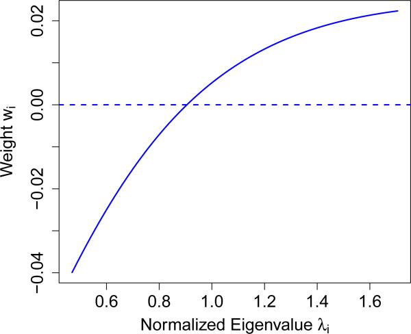
The above equation has two striking features. The first is that it depends on θ² and σ² only through the sum θ² + σ², for which we have an excellent estimator given by ${\Vert \mathit{y}\Vert }_2^2∕n$. The second feature is that it separates into the product of two terms: one term that does not depend on w, and a second term that is known (in that it contains nothing that needs to be estimated) and (strictly) convex in w. Thus we can use convex optimization to find the vector w that minimizes the upper-bound (2.7) on the variance subject to the two linear equality constraints mentioned earlier, ${\sum }_{i=1}^n{w}_i=0$ and ${\sum }_{i=1}^n{w}_i{\lambda }_i=1$, which ensure that S remains unbiased for θ². Figure 1 shows an example of such an optimized weight vector when n = 200 and p = 2000. Note that instead of just giving some positive weight to large λ_i's and some negative weight to small λ_i's, the optimal weighting is a smooth function of the λ_i. This makes sense, as the z_i's with large associated λ_i have a larger signal-to-noise ratio, and should be given greater weight. Denote the statistic S constructed using these constrained-optimal weights by T₂. Explicitly, let w* be the solution to the following convex optimization program ${\mathcal{P}}_1$:

$$\underset{\mathit{w}\in {\mathbb{R}}^n}{\arg \min }\max \left(\sum _{i=1}^n{w}_i^2,\sum _{i=1}^n{w}_i^2{\lambda }_i^2\right)\text{such that}\sum _{i=1}^n{w}_i=0,\sum _{i=1}^n{w}_i{\lambda }_i=1$$ (2.8)

and denote by $\mathrm{val}\left({\mathcal{P}}_1\right)$ the minimized objective function value. Then the statistic for our main procedure in this paper, which we call the EigenPrism procedure, is the following,

$$\begin{array}{cc}\hfill T_2& ≔\sum _{i=1}^n{w}_i^{\ast }{z}_i^2,\hfill \\ \hfill \mathbb{E}(T_2\mid \mathit{d})& ={\theta }^2,\hfill \\ \hfill \mathrm{SD}(T_2\mid \mathit{d})& \lesssim \sqrt{2\mathrm{val}\left({\mathcal{P}}_1\right)}\frac{{\Vert \mathit{y}\Vert }_2^2}{n},\hfill \end{array}$$ (2.9)

where the only approximation in the variance is the replacement of θ² + σ² by its estimator ${\Vert \mathit{y}\Vert }_2^2∕n$.

Figure 1.

Plot of weights w_i as a function of normalized eigenvalues λ_i for n = 200 and p = 2000.

With these calculations in place, we now define our (1 – α)-confidence interval for θ², by assuming that T₂ follows an approximately normal distribution (discussed later on). We construct lower and upper endpoints

$$L_{\alpha }≔\max \left(T_2-z_{1-\alpha ∕2}^{\star }\cdot \sqrt{2\mathrm{val}\left({\mathcal{P}}_1\right)}\frac{{\Vert \mathit{y}\Vert }_2^2}{n},0\right),U_{\alpha }≔T_2+z_{1-\alpha ∕2}^{\star }\cdot \sqrt{2\mathrm{val}\left({\mathcal{P}}_1\right)}\frac{{\Vert \mathit{y}\Vert }_2^2}{n},$$

where the value of L_α is clipped at zero since it holds trivially that θ² > 0, and where $z_{1-\alpha ∕2}^{\star }$ is the (1 – α/2) quantile of the normal distribution.

Remark

The idea of constructing the z_i's as contrasts has been used in the heritability literature before, e.g. Kang et al. (2008); Bonnet et al. (2014); Owen (2014), but in a strict random effects framework. In particular, when the entries of β are i.i.d. Gaussian, the z_i's become independent. With independent z_i's whose distribution depends only on the signal (θ²) and noise (σ²) parameters, the authors are able to apply maximum likelihood estimation, with associated asymptotic inference results for the signal, noise, or signal-to-noise ratio (we note that Bonnet et al. (2014) generalize such estimators somewhat to the case of a Bernoulli-Gaussian random effects model). The crucial difference between our work and theirs is that we make no assumptions (e.g., Gaussianity, sparsity) on the coefficient vector, and thus not only are the z_i's not independent in our setting, but their dependence (and thus the full likelihood) is a function of the products β_iβ_j, and thus a maximum likelihood approach in this setting would still be overparameterized.

Next, we discuss the coverage and width properties of this constructed confidence interval.

2.2.2 Coverage

Now that we are equipped with an unbiased estimator and a computable variance (upper-bound), and have constructed a confidence interval (CI) using a normal approximation, there are two main questions to answer in order to determine whether these CIs will exhibit the desired coverage properties. In particular, we would like to know if substituting θ² + σ² with ${\Vert \mathit{y}\Vert }_2^2∕n$ substantially affects the variance formula, and we would like to know if T₂ is approximately normally distributed (so that we can construct arbitrary CIs from just the second moment). For the first question, since ${\Vert \mathit{y}\Vert }_2^2$ is a rescaled ${\chi }_n^2$ random variable, for nominal coverage of 1 – α, the coverage actually achieved can be closely approximated by $\mathbb{P}\{\mid N(0,1)\mid \le z_{1-\alpha ∕2}\cdot {\chi }_n^2∕n\}$ (where the N(0, 1) and the ${\chi }_n^2$ are independent), assuming exact normality. Table 1 shows that for nominal 95% coverage, one would need fewer than 20 samples to achieve less than 90% coverage. For the second question, the following theorem establishes the asymptotic normality of T₂.

Table 1.

Values of $\mathbb{P}\{\mid N(0,1)\mid \le z_{0.975}\cdot {\chi }_n^2∕n\}$ for a range of n.

n	10	20	50	100	500	1000	5000
Coverage	87.5%	91.0%	93.3%	94.1%	94.8%	94.9%	95.0%

Theorem 1

Under the linear model (1.1) with Gaussian random design and errors given in Equation (1.4), the estimator T₂ as defined in Equation (2.9) is asymptotically normal as n, p → ∞ and n/p → γ ∈ (0, 1). This holds for any values of θ² and σ², including values that vary with n. Explicitly,

$$\frac{T_2-{\theta }^2}{\mathrm{SD}(T_2\mid d)}\stackrel{d}{\to }N(0,1).$$

Proof

The proof is given in Appendix C.

For finite-sample results, we defer to the simulation results of Section 3.1 to show that for problems of reasonable size $(\min \{n,p\}\gtrsim 100)$, CIs constructed as if T₂ were exactly normal with variance exactly given by Equation (2.9) never result in below-nominal coverage.

2.2.3 Width

Once we have confirmed that our CIs provide the proper coverage, the next topic of interest is their widths. It is not hard to obtain a closed-form asymptotic upper-bound for Var(T₂) (the details are worked out in Appendix D). In particular, letting Y_γ denote a random variable with Marčenko–Pastur (MP) distribution with parameter γ (Marčenko and Pastur, 1967), and M_γ denote the median of Y_γ, define the constants,

$$\begin{array}{cc}\hfill A_{\gamma }& =\mathbb{E}[Y_{\gamma }\cdot (1_{Y_{\gamma }\ge M_{\gamma }}=1_{Y_{\gamma }<M_{\gamma }})],\hfill \\ \hfill B_{\gamma }& =\mathbb{E}\left(Y_{\gamma }^2\right).\hfill \end{array}$$ (2.10)

Then in the limit as n, p → ∞ and n/p → γ ∈ (0, 1),

$$\sqrt{n}\cdot \frac{\sqrt{\mathrm{Var}\left(T_2\right)}}{{\theta }^2+{\sigma }^2}\le \sqrt{2}\cdot \max \left(\frac{1}{A_{\gamma }},\frac{\sqrt{B_{\gamma }}}{A_{\gamma }}\right).$$ (2.11)

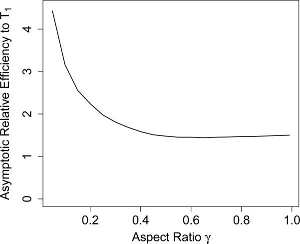
We can draw a few conclusions from Equation (2.11). The most obvious is that for n, p → ∞, n/p → γ ∈ (0, 1), σ² asymptotically bounded above and θ² asymptotically bounded below, the error of T₂, as a fraction of its estimand θ², converges to 0 in probability at a rate of n^−1/2. Note that we make no assumptions at all on the structure of β, and just require that θ² does not asymptote at 0. The equation also lets us compute a conservative upper-bound on the asymptotic relative efficiency (ARE), defined as the asymptotic ratio of standard deviations (although it is often defined by variances elsewhere), of T₂ with respect to T₁ from Section 2.1 (see (2.2)), the latter of which uses exact knowledge of σ² and has standard deviation characterized by the ${\chi }_n^2$ distribution. While we may not be able to formulate a closed-form expression for it in terms of expectations due to the constrained minimization functional, the standard deviation bound for T₂ in Equation (2.9) will also converge to a constant times SD(T₁) under the same asymptotic conditions, where the constant depends only on the MP distribution. This is because the optimal weights are a smooth function of the λ_i. Due to fast convergence to the MP distribution, we can numerically approximate this exact asymptotic ratio. Figure 2 shows this estimate of the ARE of T₂ to T₁ as a function of γ. Note that the standard deviation bound for T₂ in Equation (2.9), used to compute the curve in Figure 2, is still an upper-bound for the ARE of T₂ with respect to T₁, but it reflects the ratio of CI widths between the EigenPrism procedure and a CI constructed from T₁ with knowledge of σ². The figure demonstrates how close in width the EigenPrism procedure comes to an exact CI for T₁ which knows σ². In particular, for γ ≳ 0.25, the EigenPrism CIs are at most twice as wide as those for T₁.

Figure 2.

Estimate of the asymptotic relative efficiency of T₂ to T₁.

Another notable feature of Figure 2 is how large the ARE becomes as γ → 0. This is a symptom of an important property of not just our procedure, but the frequentist problem as a whole. First, it is clear that if all the λ_i ≡ 1, our procedure fails, as the $z_i^2$ no longer provide any contrast between θ² and σ², and no linear combination of them will produce an unbiased statistic for θ². Intuitively, note that $\mathbb{E}\left(z_i^2\right)\propto {\lambda }_i\rho +(1-\rho )$, so that the problem of estimating ρ is that of estimating the slope and intercept of a regression line. But in regression, when the predictor variable assumes a constant value, as it would when λ_i ≡ 1, it becomes impossible to estimate the slope and intercept. To understand better how our procedure performs when the spread of the λ_i approaches zero, consider the case when λ₁ = ··· = λ_n/2 = 1 + a and λ_n/2+1 = ··· = λ_n = 1 – a. In this case SD(λ_i) = a, and it is easy to show that

$$\mathrm{val}\left({\mathcal{P}}_1\right)=\frac{1+a^2}{a^{2}n},$$

so if $\sqrt{n}\mathrm{SD}\left({\lambda }_i\right)\to 0$, then a²n → 0 and so $\mathrm{val}\left({\mathcal{P}}_1\right)\to \infty$.

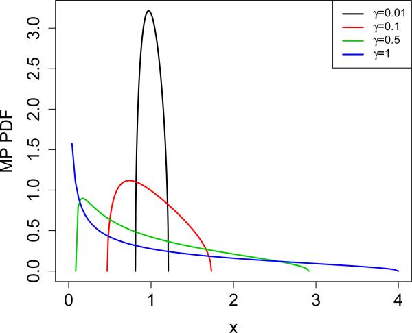
Returning to our original model in which X is i.i.d. N(0, 1), the λ_i's will be approximately MP-distributed with parameter γ = n/p. Figure 3 shows visually how the width of the MP distribution depends on γ, and analytically, SD(Y_γ) = √γ. We show in the following theorem (proved in Appendix E) that if the λ_i's are too close to 1 and n << p, it is impossible for any procedure to reliably distinguish between the case of ρ = 0 (pure noise) and ρ = 1/2 (variance equally split between signal and noise).

Figure 3.

Probability density function (PDF) of Marčenko–Pastur distribution for various values of γ.

Theorem 2

Let p ≥ n ≥ 1. Suppose that

$$\mathit{Z}=\theta \cdot {\mathit{DV}}^{\mathsf{T}}\mathit{a}+\sigma \cdot \epsilon$$ (2.12)

where θ < 0, σ < 0, and a unit vector a are all fixed but unknown, $\mathit{D}\in {\mathbb{R}}^{n\times n}$ is a known nonnegative diagonal matrix with ${\sum }_{i=1}^n{\lambda }_i≔{\sum }_{i=1}^2{D}_{ii}^2∕p=n$, $\mathit{V}\in {\mathbb{R}}^{p\times n}$ is a random Haar-distributed orthonormal matrix, and ε ~ N(o, I_n) independent of V. Consider the simple scenario where we are trying to distinguish between only two possibilities, denoted by distributions P₀ and P₁:

$$P_0:\mathit{Z}follows\left(2.12\right)with\theta =0and\sigma =1,vs.P_1:\mathit{Z}follows\left(2.12\right)with\theta =\sigma =\frac{1}{\sqrt{2}}.$$

Then for any test $\psi :{\mathbb{R}}^n\to \{0,1\}$, the power to correctly distinguish between these two distributions is bounded as

$${\mathbb{P}}_{\mathit{Z}\sim P_0}[\psi \left(\mathit{Z}\right)=1]+{\mathbb{P}}_{\mathit{Z}\sim P_1}[\psi \left(\mathit{Z}\right)=0]\ge 1-\left(\sqrt{\frac{{\sum }_{i=1}^n{({\lambda }_i-1)}^2}{8}}+\sqrt{\frac{n∕p}{4\pi }}\right).$$

In other words, every test ψ has high error, with

$$\mathbb{P}\left(\text{Type I error}\right)+\mathbb{P}\left(\text{Type II error}\right)\ge 1-\left(\sqrt{\frac{{\sum }_{i=1}^n{({\lambda }_i-1)}^2}{8}}+\sqrt{\frac{n∕p}{4\pi }}\right),$$

so that if the λ_i are tightly distributed around 1 and n << p, the problem of estimating ρ, and thus θ, is extremely difficult. Note that for approximately MP-distributed λ_i with γ = n/p ≈ 0, both ${\sum }_{i=1}^n{({\lambda }_i-1)}^2$ and n/p are quite small, explaining the spike in ARE in Figure 2 as γ → 0.

Another way to evaluate how short the EigenPrism CIs are, compared to how short they could be, is to compare to a Bayesian procedure on a Bayesian problem. This is done in Section 3.1.

2.2.4 Computation

As a procedure intended for use in high-dimensional settings, it is of interest to know how the EigenPrism procedure scales with large problem dimensions. There are essentially two parts to the procedure: the SVD, and the optimization (2.8) to choose w*. Due to the strict convexity of the optimization problem, it is extremely fast to solve (2.8) and in all of our simulations the runtime was dominated by the SVD computation. In Appendix F we include a snippet of Matlab code in the popular convex optimization language CVX (Grant and Boyd, 2014, 2008) that reformulates the optimization problem (2.8) as a second-order cone problem. Even if the optimization becomes extremely high-dimensional, note that the optimal weights w* are a smooth function of their associated eigenvalues λ_i. Thus we can approximate w* extremely well by subsampling the λ_i, computing a lower-resolution optimal weight vector, and then linearly interpolating to obtain the higher-resolution, high-dimensional w*. For the SVD, note that V never needs to be computed. Thus, the computation scales as n²p with a small constant of proportionality, as the SVD of ${\mathit{XX}}^{\mathsf{T}}$ is all that is needed.

3 Derivative Procedures

In this section, we go into more detail about the three related problems of performing inference on estimation error of a high-dimensional regression estimator, noise level in a high-dimensional linear model, and genetic signal-to-noise ratio, including simulation results. MATLAB code for the numerical results in this paper is available on the first author's website.

3.1 High-Dimensional Regression Error

We have already shown in Section 1.2 that the problem of inference for high-dimensional regression error is equivalent, with a change of variables, to that of inference on θ. Under assumptions (1.4), our framework even allows for selection of a subset of $\widehat{\beta }$, for instance if the doctor sees an anomaly in a region of the reconstructed image, he or she may only care about error in that region. In that case, for a subset of indices R (with corresponding complement R^c), Equation (1.3) can be rewritten as

$$\tilde{\mathit{y}}={\mathit{X}}_R^{\left(1\right)}({\beta }_R-{\widehat{\beta }}_R)+{\mathit{X}}_{R^c}^{\left(1\right)}({\beta }_{R^c}-{\widehat{\beta }}_{R^c})+\epsilon ={\mathit{X}}_R^{\left(1\right)}({\beta }_R-{\widehat{\beta }}_R)+\tilde{\epsilon },$$

where $\tilde{\epsilon }$ is an i.i.d. Gaussian vector independent of ${\mathit{X}}_R^{\left(1\right)}$, so that defining $\theta ={\Vert {\beta }_R-{\widehat{\beta }}_R\Vert }_2$ puts this problem squarely into the EigenPrism framework, regardless of the fact that R may be chosen after observing $\widehat{\beta }$ (recall that $\widehat{\beta }$ was fitted on an independent subset of the data, (X⁽⁰⁾, y⁽⁰⁾)).

We note that the requirement that the columns of X be independent in order to perform inference on ${\Vert \widehat{\beta }-\beta \Vert }_2^2$ cannot be relaxed. However, with a known covariance Σ, one could instead perform inference on ${\Vert {\Sigma }^{1∕2}(\widehat{\beta }-\beta )\Vert }_2^2$. Of course, inference for either ${\Vert \widehat{\beta }-\beta \Vert }_2^2$ or ${\Vert {\Sigma }^{1∕2}(\widehat{\beta }-\beta )\Vert }_2^2$ is sufficient if the ultimate goal is to invert the CI to test a global null hypothesis on the coefficient vector.

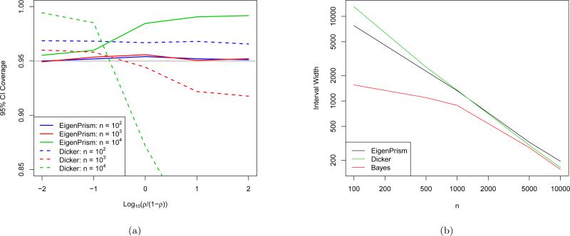
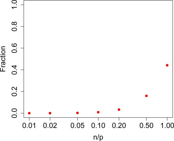
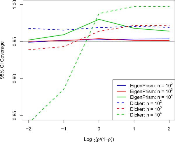
What remains to be seen then is (1) that coverage is not lost by approximating θ² + σ² by ${\Vert \mathit{y}\Vert }_2^2$ and by assuming T₂ is normal, and (2) how short the resulting CIs are relative to how short they could be. To investigate (1), we fixed p at 10⁴, θ² + σ² = 10⁴, varied n on a log scale between 0 and p, and varied ρ (recall Equation 2.6) between 0 and 1 by taking equally spaced values of log(ρ/(1 – ρ)). Note that due to rotational symmetry, the direction of β is irrelevant. We ran 10⁴ simulations of the EigenPrism procedure to generate 95% CIs and compared coverage across the settings in Figure 4(a). We also simulated CIs using the results of Dicker (2014) by simply plugging in its estimators for θ² and σ² to its asymptotic variance formula (which depends on the exact parameters). Note that the EigenPrism CIs achieve at least nominal coverage in all cases, while the Dicker procedure is less reliable, especially for large ρ. One setting in which we see EigenPrism over-cover is when n ≈ p and ρ ≈ 1. This can be explained by the variance upper-bound for T₂ in Equation (2.5), which is tight when p is large and ${\left(p{\sum }_{i=1}^n{\left(w_i^{\ast }{\lambda }_i\right)}^2\right)}^{-1}\ll 1$. Figure 5 shows that, except when n ≈ p, we indeed have ${\left(p{\sum }_{i=1}^n{\left(w_i^{\ast }{\lambda }_i\right)}^2\right)}^{-1}\ll 1$.

Figure 4.

(a) Coverage of 95% EigenPrism and Dicker confidence intervals as a function of ρ for p = 10⁴ and θ² + σ² = 10⁴. (b) EigenPrism confidence interval, Dicker confidence interval, and Bayes credible interval widths as a function of n for p = 10⁴ and β sampled according to the Bayesian model in Equation (G.1).

Figure 5.

Plot of the fraction $\frac{1}{p{\sum }_{i=1}^n{\left(w_i^{\ast }{\lambda }_i\right)}^2}$ as a function of n/p (on the log scale) for p = 10⁴.

To investigate (2), we simulated the EigenPrism procedure on a Bayesian model and compared the EigenPrism widths to those obtained by computing equal-tailed Bayes credible intervals (BCI) from a Gibbs-sampled posterior. The details of the Bayesian setup are given in Appendix G, but the resulting CI widths are summarized in Figure 4(b) for p = 10⁴ and a range of n. Again, we also compared to Dicker CIs. Each point on the plot represents 1000 simulations. Although the Dicker CIs become slightly shorter than EigenPrism's for large n, we note (as evidenced by Figure 4(a)) that this is exactly the regime in which the Dicker CIs have unreliable coverage. We will see later in Section 4.1 that even for small n and ρ, the Dicker CIs quickly lose coverage as correlations are added to the design matrix, while EigenPrism's coverage is in fact quite robust. The other salient features of this plot are that the EigenPrism CI widths decrease at a steady √n-rate, while the BCI widths start much lower and appear to asymptote around the EigenPrism CI width curve. The fact that the BCI widths are much shorter for small n can be explained by the information contained in the priors, which is important for two reasons. In any frequentist-Bayesian comparison of methods, there is always the phenomenon that small n means the data contains little information, so the prior information given to the Bayesian method makes it heavily favored over the frequentist method. However, as we saw in Section 2.2.3, the frequentist problem is fundamentally limited not just by n but by SD(λ_i) as well, and here since p is fixed, small n corresponds to small SD(λ_i) as well, adding an extra layer of challenge for the EigenPrism procedure. As n increases though, the BCIs rely more heavily on the data, and come much closer in width to the EigenPrism CIs, with the average relative width increase bottoming-out at about 5% for n = 5000. The relative uptick in the EigenPrism CI widths for n ≈ p can again be explained by the upper-bound in Equation (2.5).

3.2 Inference on σ²

We can use almost exactly the same EigenPrism procedure for σ² as we did for θ². Recall Equation (2.3),

$$\mathbb{E}(S\mid \mathit{d})={\theta }^2\sum _{i=1}^n{w}_i{\lambda }_i+{\sigma }^2\sum _{i=1}^n{w}_i.$$

To make S unbiased for θ², we constrained ${\sum }_{i=1}^n{w}_i=0$ and ${\sum }_{i=1}^n{w}_i{\lambda }_i=1$. However by switching these linear constraints, so that ${\sum }_{i=1}^n{w}_i=1$ and ${\sum }_{i=1}^n{w}_i{\lambda }_i=0$, we make S unbiased for σ². The variance formulae and upper-bounds in Equations (2.4)–(2.7) still hold, so that we can construct T₃ (and an associated CI). Let w** be the solution to the following convex optimization program ${\mathcal{P}}_2$:

$$\underset{\mathit{w}\in {\mathbb{R}}^n}{\arg \min }\max \left(\sum _{i=1}^n{w}_i^2,\sum _{i=1}^n{w}_i^2{\lambda }_i^2\right)\text{such that}\sum _{i=1}^n{w}_i=1,\sum _{i=1}^n{w}_i{\lambda }_i=0$$

and denote by $\mathrm{val}\left({\mathcal{P}}_2\right)$ the minimized objective function value. Then the EigenPrism procedure for performing inference on σ² reads

$$\begin{array}{cc}\hfill T_3& ≔\sum _{i=1}^n{w}_i^{\ast \ast }{z}_i^2,\hfill \\ \hfill \mathbb{E}(T_3\mid \mathit{d})& ={\sigma }^2,\hfill \\ \hfill \mathrm{SD}(T_3\mid \mathit{d})& \lesssim \sqrt{2\mathrm{val}\left({\mathcal{P}}_2\right)}\frac{{\Vert \mathit{y}\Vert }_2^2}{n},\hfill \end{array}$$

where again, the only approximation in the variance is the replacement of θ² + σ² by its estimator ${\Vert \mathit{y}\Vert }_2^2∕n$. The analogue to Theorem 1 holds and is proved in Appendix C:

$$\frac{T_3-{\sigma }^2}{\mathrm{SD}(T_3\mid d)}\stackrel{d}{\to }N(0,1).$$

Finally, as before, we construct the lower and upper endpoints to obtain an approximate (1 – α)-CI for σ² via

$$L_{\alpha }≔\max \left(T_3-z_{1-\alpha ∕2}^{\star }\cdot \sqrt{2\mathrm{val}\left({\mathcal{P}}_2\right)}\frac{{\Vert \mathit{y}\Vert }_2^2}{n},0\right),U_{\alpha }≔T_3+z_{1-\alpha ∕2}^{\star }\cdot \sqrt{2\mathrm{val}\left({\mathcal{P}}_2\right)}\frac{{\Vert \mathit{y}\Vert }_2^2}{n}.$$

Note that if the columns of X have a known covariance matrix Σ, the exact same machinery goes through by replacing X by XΣ^−1/2 and replacing β by Σ^1/2β.

Turning to simulations, we aim to show that the EigenPrism CIs for σ² have at least nominal coverage. We take the same setup as in Figure 4(a) but instead construct 95% CIs for σ². Figure 6 shows the result, and as before we see that EigenPrism's coverage never dips below nominal levels in any of the settings, while for small ρ the Dicker CI's coverage can be unreliable, especially for large n. We performed a similar experiment with a Bayesian model to compare EigenPrism CI widths for σ² with those of equal-tailed BCIs, but found a less-desirable comparison than in the θ case. In particular, the most favorable simulations showed the EigenPrism CI approximately 30% wider than the BCI, which can likely be attributed to the more-informative prior (Inverse Gamma) on σ² than that on θ² (nearly Exponential) in the Bayesian model (G.1). Although we would have liked to try an Exponential prior for σ², due to a lack of conjugacy the resulting Gibbs sampler was computationally intractable. We note that except in special cases, it can be very computationally challenging to construct BCIs, especially in high dimensions.

Figure 6.

Coverage of 95% EigenPrism and Dicker confidence intervals for σ² as a function of ρ for p = 10⁴ and θ² + σ² = 10⁴. Each point represents 10⁴ simulations, and the grey line denotes nominal coverage.

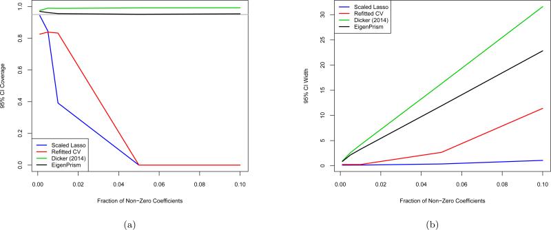
We point out that only two other σ² estimators in the literature provide any inference results, namely the scaled Lasso (Sun and Zhang, 2012) and the refitted cross validation (CV) method of Fan et al. (2012). In particular, under some sparsity conditions on the coefficient vector, the authors find aymptotic normal approximations to their estimators. To compare our CIs with theirs, we compared them on the same simulations, but quickly found that scaled Lasso and refitted CV CIs only achieve nominal coverage in extremely sparse settings. We also compared the plug-in CI for the estimator in Dicker (2014). This coverage comparison is shown in Figure 7(a). The scaled Lasso CIs only achieve nominal coverage when 1 out of the 1000 coefficients are non-zero, and quickly drop off to less than half of nominal coverage by 1% sparsity. The refitted CV CIs undercover by about 10% even in the sparsest settings, and also fall off further in coverage as sparsity decreases. The EigenPrism and Dicker CIs achieve at least nominal coverage at all sparsity levels examined. Figure 7(b) shows average CI widths for the same simulations. The much smaller widths of the scaled Lasso and refitted CV CIs align with their lack of coverage, reflecting the fact that the bias and variance of their estimators can be poorly characterized in finite samples. The Dicker CIs are consistently wider than EigenPrism's, with the inflation factor nearly 40% at the right-hand side of the plot.

Figure 7.

(a) Coverage and (b) width of scaled lasso, refitted cross validation, plug-in CI from Dicker (2014) described in Section 3.1, and EigenPrism confidence intervals when n = 500, p = 1000, σ² = 1, and non-zero entries of β equal to 1. Each point represents 10⁴ simulations, and the grey line denotes nominal coverage.

3.3 Genetic Variance Decomposition

Consider a linear model for a centered continuous phenotype (y_i) such as height, as a function of a centered SNP array (x_i). The variance can be decomposed as

$$\mathbb{E}\left(y_i^2\right)=\mathbb{E}\left[{\left({\mathit{x}}_i^{\mathsf{T}}\beta \right)}^2\right]+{\sigma }^2.$$ (3.1)

Under linkage disequilibrium, assuming column-independence is unrealistic. However, a wealth of genomic data has resulted in this column dependence possibly being estimable from outside data sets (e.g. Abecasis et al. (2012)), so we may instead take ${\mathit{x}}_i\stackrel{i.i.d.}{\sim }N(0,\Sigma )$ with Σ known (we will discuss a relaxation of the normality in Section 4.1). Then Equation (3.1) reduces to

$$\mathbb{E}\left(y_i^2\right)={\Vert {\Sigma }^{1∕2}\beta \Vert }_2^2+{\sigma }^2,$$

which provides a formula for the linear model's signal-to-noise ratio,

$$\mathrm{SNR}=\frac{{\Vert {\Sigma }^{1∕2}\beta \Vert }_2^2}{{\Vert {\Sigma }^{1∕2}\beta \Vert }_2^2+{\sigma }^2}.$$

The SNR is connected to the genetic heritability in that, for the simplified approximation to a linear model with additive i.i.d. noise, it quantifies what fraction of a continuous phenotype's variance can be explained by SNP data. We note that there are many different definitions of heritability, and the SNR aligns most closely with the narrow-sense, or additive, heritability, as we do not allow for interactions or dominance effects. The extent of the connection between the two definitions depends on how complete the SNP array is—if every SNP is measured, they correspond exactly.

Although until now we have been working with ${\Vert \beta \Vert }_2^2$, while the SNR estimation problem seems to call for ${{\Sigma }^{1∕2}\beta \Vert }_2^2$, the above problem turns out to fit right into our framework. Explicitly, the linear model can be rewritten as

$$\mathit{y}=\left(\mathit{X}{\Sigma }^{-1∕2}\right)\left({\Sigma }^{1∕2}\beta \right)+\epsilon ,$$

where now the rows of (XΣ^−1/2) are i.i.d. N(0, I), and θ² corresponds to the new quantity of interest: ${\Vert {\Sigma }^{1∕2}\beta \Vert }_2^2$. Since $\mathbb{E}({\Vert \mathit{y}\Vert }_2^2∕n)={\Vert {\Sigma }^{1∕2}\beta \Vert }_2^2+{\sigma }^2$ now, applying our methodology to XΣ^−1/2 gives a natural estimate for SNR, namely,

$$\widehat{\mathrm{SNR}}≔\frac{T_2}{{\Vert \mathit{y}\Vert }_2^2∕n}.$$

Continuing, as we have done throughout this paper, to treat ${\Vert {\Sigma }^{1∕2}\beta \Vert }_2^2+{\sigma }^2$ as if it is known and equal to ${\Vert \mathit{y}\Vert }_2^2∕n$, our distributional results for T₂ extend to give us an approximate confidence interval for $\widehat{\mathrm{SNR}}$.

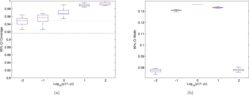
We turn again to simulations to demonstrate the performance of the EigenPrism procedure described above for constructing SNR CIs. One major consideration is that of course, SNP data is discrete, not Gaussian. However, we will show in Section 4.1 that the EigenPrism procedure works well empirically even under non-Gaussian marginal distributions. Here, we run experiments for n = 10⁵, p = 5 × 10⁵, θ² + σ² = 10⁴, Bernoulli(0.01) design with independent columns, β having 10% non-zero entries, and SNR varying from nearly 0 to nearly 1. Figure 8 shows the EigenPrism CI coverage and average widths. Note that although our CIs are conservative, we never lose coverage, and at worst our 95% CI would give the SNR to within an error of ±6.8%.

Figure 8.

(a) Coverage, and (b) average widths, of EigenPrism SNR 95% confidence intervals. Experiments used n = 10⁵, p = 5×10⁵, θ² + σ² = 10⁴, Bernoulli(0.01) design, and β with 10% non-zero, Gaussian entries. Each boxplot summarizes the (a) coverage and (b) width for 20 different β's, each of which is estimated with 500 simulations. The whiskers of the boxplots extend to the maximum and minimum points. The black dotted line in (a) is the 95% confidence lower-bound for the lowest whisker in each plot assuming all CIs achieve exact coverage, and the grey line shows nominal coverage.

4 Robustness and 2-Step Procedure

In this section we follow up our investigation of the EigenPrism framework by considering its robustness to model misspecification and presenting a 2-step procedure that can improve the CI widths of the vanilla EigenPrism procedure.

4.1 Robustness

An important practical question is how robust the EigenPrism CI is to model misspecification. In particular, our theoretical calculations made some fairly stringent assumptions, and we explore here their relative importances. Some standard assumptions that we rely on are that the model is indeed linear and the noise is i.i.d. Gaussian and independent of the design matrix. These assumptions are all present, for instance, in OLS theory, and we assume that problems substantially deviating from satisfying them are not appropriate for our procedure. As explained in Section 1.2, the random design assumption is necessitated by the high-dimensionality (p > n) of our problem, and within the random design paradigm, the assumption of i.i.d. rows is still broadly applicable, for instance whenever the rows represent samples drawn independently from a population.

The not-so-standard assumption we make is that the columns of X are also independent, and all of X's entries are N(0, 1) (note that each column of a real design matrix can always be standardized so that at least the first two marginal moments match this assumption). These assumptions are important because they ensure that the columns of V are uniformly distributed on the unit sphere, so that we can characterize both the expectation and variance of their inner product with β. Although we will see that the marginal distribution of the elements of X is not very important as long as n and p are not small, in general the independence of the columns is crucial. We note that there is work in random matrix theory showing that for certain random matrices which are not i.i.d. Gaussian, the eigenvectors are still in some sense asymptotically uniformly distributed on the unit sphere (see for example Bai et al. (2007)). This suggests that EigenPrism CIs, at least asymptotically, may work well in a broader context than shown so far.

Before explaining further, we feel it is important to recall that for two of the three inference problems this work addresses (inference for σ² and signal-to-noise ratio), the EigenPrism procedure extends to easily account for any known covariance matrix among the columns of X. However in the vanilla example of simply constructing CIs for θ², correlation among the columns of X can cause serious problems. To first order, we need $\mathbb{E}({\Vert {\mathit{V}}^{\mathsf{T}}\beta \Vert }_2^2\mid \mathit{d})\approx {\theta }^{2}n∕p$, or else T₂ will be biased and the resulting shifted interval will have poor coverage. From a practical perspective, unless β is adversarially chosen, it may seem unlikely that β will be particularly aligned or misaligned (orthogonal) to the directions in which X varies. In particular, if we make a random effects assumption and say that the entries of β are i.i.d. N(0, τ²), then the EigenPrism procedure will achieve nominal coverage. A slightly more subtle problem occurs if β is chosen not adversarially, but sparse in the basis of X's principal components. In this case, although T₂ is approximately unbiased, the variance estimate could be far too small, resulting again in degraded coverage.

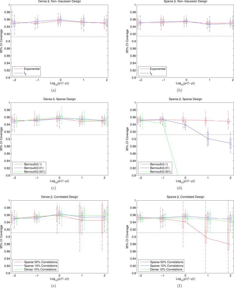
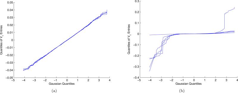
To investigate how wrong the model has to be to make our CIs undercover, we construct EigenPrism CIs on data coming from models not satisfying our assumptions. In particular, we ran the EigenPrism procedure on design matrices with either i.i.d. entries with very different higher-order moments than a Gaussian, i.i.d. entries that were sparse, or Gaussian entries and correlated columns. Since the direction of β becomes relevant in all these cases, we performed experiments with both dense and sparse β, and in each regime measured coverage for 20 different β's. The results of simulations with n = 10³, p = 10⁴, and θ² + σ² = 10⁴ are plotted in Figure 9. Each boxplot summarizes the coverage for 20 different β's, each of which is estimated with 500 simulations. The whiskers of the boxplots extend to the maximum and minimum points, and the black dotted line is the 95% confidence lower-bound for the lowest whisker in each plot assuming all CIs achieve exact coverage. As can be seen from Figures 9(a) and 9(c), when β is dense, the marginal moments and sparsity of the entries of X do not affect coverage. Figures 9(e) and 9(f) show that even small unaccounted-for correlations among the columns of X do not greatly affect coverage, although larger correlations, as expected, can result in serious undercoverage for certain β's. As a comparison, we also simulated the Dicker CIs in the setting of Figures 9(e) and 9(f), wherein coverage never exceeded 40% for any β or correlation structure. Figures 9(b) and 9(d) show that when β is sparse, coverage is much more sensitive to sparsity in X, although if X is not sparse, coverage remains robust to higher-order moments of the design matrix. Figure 10 demonstrates the crucial difference when X is sparse by showing a few realizations of quantile-quantile plots comparing the distribution of the entries of V₁ to a Gaussian distribution, for Bernoulli(0.1)- and Bernoulli(0.001)-marginally-distributed X. The figure shows that the distribution for Bernoulli(0.1) is very nearly Gaussian, but that this is far from the case for Bernoulli(0.001), and thus it is the problem described at the end of the preceding paragraph that causes problems.

Figure 9.

The first column of plots ((a), (c), (e)) generates ${\beta }_i\stackrel{i.i.d.}{\sim }N(0,1)$ and renormalizes to control θ², while the second column of plots ((b), (d), (f)) does the same but then sets 99% of the β_i to zero before renormalizing. The first two rows of plots ((a), (b), (c), (d)) use X_ij i.i.d. from some non-Gaussian distribution renormalized to have mean 0 and variance 1. The third row of plots ((e), (f)) uses marginally standard Gaussian X but with correlations among the columns; see Appendix H for detailed constructions. See text for detailed boxplot constructions and interpretation of the dashed line.

Figure 10.

Quantile-quantile plots measuring the Gaussianity of 5 realizations of the entries of V₁ for (a) Bernoulli(0.1)-distributed X and (b) Bernoulli(0.001)-distributed X.

4.2 2-Step Procedure

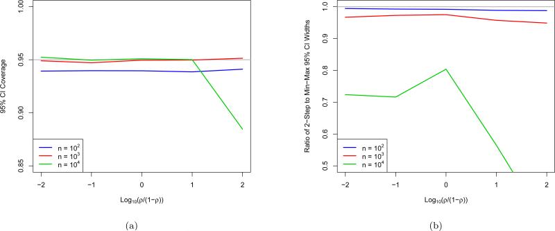
Note that in the variance upper-bound of Equation (2.7), the unknown ρ is maximized over to remove it from the equation. This leads not only to conservative CIs, but suboptimal w* as well, since w* are obtained by minimizing this upper-bound, as opposed to the more accurate function of ρ. However by the end of the EigenPrism procedure, we have produced estimates of both θ and θ² + σ², suggesting the possibility of a 2-step plug-in procedure to remove the need for the upper-bound in Equation (2.7). Explicitly, in the first step, we run the EigenPrism procedure to obtain an estimate $\widehat{\rho }=T_2∕({\Vert \mathit{y}\Vert }_2^2∕n)$ of ρ. In the second step, we re-run the procedure treating $\rho =\widehat{\rho }$ as known, and thus minimize the bound (2.5) to compute w* . Although the 2-step procedure indeed produces shorter CIs than the EigenPrism procedure, it does not achieve nominal coverage with the same consistency, as shown in Figure 11.

Figure 11.

(a) Coverage and (b) width relative to EigenPrism of 2-step confidence intervals for p = 10⁴ and θ² + σ² = 10⁴ across a range of ρ and n, with each point representing 10⁴ simulations. Grey lines show (a) nominal coverage and (b) reference ratio of 1.

There are two particularly surprising aspects of this plot. The first is that the 2-step procedure produces substantial gains in width even for ρ values near 0 and 1. This is surprising because the upper-bound (2.7) that is eliminated by the 2-step procedure is tight when ρ is nearly 0 or 1, however it is still not exact. The slightly loose variance upper bound turns out to have an optimizing w that is substantially different from the exact variance formula. The second surprising feature is that the width improvement is in fact smallest for ρ not near the endpoints 0 or 1. This can be explained by the clipping at 0. For ρ ≈ 0, most CIs, both EigenPrism and 2-step, are cut nearly in half by clipping, so the fractional width improvement achieved by the 2-step procedure is fully realized. For ρ ≈ 1, both intervals are rarely clipped, and again the 2-step procedure realizes its full width improvement. However, for ρ not close to 0 or 1, many EigenPrism CIs are only slightly shrunk by clipping, so that the shorter 2-step intervals shorten the right side of the interval but leave the unclipped left side about the same, so that much less than the full width improvement is realized.

Although the 2-step procedure can provide substantial gains in width, it loses the robustness of the EigenPrism procedure, as shown in the slight undercoverage for n = 100 and the substantial undercoverage for large ρ and n = p. Therefore, in practice, we recommend use of the 2-step procedure instead of the EigenPrism procedure when n ≉ p or when the statistician is confident that ρ is not close to 1.

5 Variance Decomposition in the Northern Finland Birth Cohort

We now briefly show the result of applying EigenPrism to a dataset of SNPs and continuous phenotypes to perform inference on the $\mathrm{SNR}={\Vert {\Sigma }^{1∕2}\beta \Vert }_2^2∕({\Vert {\Sigma }^{1∕2}\beta \Vert }_2^2+{\sigma }^2)$. The data we use comes from the Northern Finland Birth Cohort 1966 (NFBC1966) (Sabatti et al., 2009; Järvelin et al., 2004), made available through the dbGaP database (accession number phs000276.v2.p1). The data consists of 5402 SNP arrays from subjects born in Northern Finland in 1966, as well as a number of phenotype variables measured when the subjects were 31 years old. After cleaning and processing the data (the details of which are provided in Appendix I), 328,934 SNPs remained. The resulting 5402 × 328, 934 design matrix X contained approximately 58% 0's (homozygous wild type), 34% 1's (heterozygous), and 8% 2's (homozygous minor allele).

In order to use EigenPrism directly, we would need to know Σ, as simply using I_p presents two possible problems:

• (1)If X is not whitened before taking the SVD, the columns of V may be far from Haar-distributed, rendering our bias and variance computations incorrect.
• (2)If Σ = I_p, then the ostensible target of our procedure is ${\Vert \beta \Vert }_2^2∕({\Vert \beta \Vert }_2^2+{\sigma }^2)$, which may differ substantially from $\mathrm{SNR}={\Vert {\Sigma }^{1∕2}\beta \Vert }_2^2∕({\Vert {\Sigma }^{1∕2}\beta \Vert }_2^2+{\sigma }^2)$.

Unfortunately, the problem of estimating the covariance matrix of a SNP array is extremely challenging (and the subject of much current research) due to the fact that n << p, even if we use outside data, so we prefer to avoid it here. In order to simply treat the covariance matrix as diagonal, we must consider the two problems above. There is a widely-held belief that the SNP locations that are important for any given trait are relatively rare (see, for example, Yang et al. (2010); Golan and Rosset (2011)), and thus spaced far enough apart on the genome to be treated as independent. This precludes problem (2) above, since with nonzero coefficients spaced far apart, we have ${\Vert {\Sigma }^{1∕2}\beta \Vert }_2^2\approx {\Vert \beta \Vert }_2^2$ (we take the columns of X to be standardized, so the diagonal of Σ is all ones). For problem (1), we know that far apart SNPs are very nearly independent, so we may expect that the true Σ is roughly diagonal, and we already showed in Section 4.1 that the EigenPrism procedure is robust to some small unaccounted-for covariances when constructing CIs for ${\Vert \beta \Vert }_2^2$. To ensure that problems (1) and (2) do not cause EigenPrism to break down, we perform a series of diagnostics before applying it to the real data.

Given the approximation of Σ as diagonal, we first performed a series of simulations to ensure EigenPrism's accuracy was not affected. Specifically, we ran the EigenPrism procedure (with adjustments described in the paragraph below) on artificially-constructed traits, but using the same standardized design matrix X from the NFBC1966 data set. For 20 different β vectors, we generated 500 independent Gaussian noise realizations and recorded the coverage of 95% EigenPrism CIs for SNR. The noise variance was 1, and the β's were chosen to have 300 nonzero entries with uniformly distributed positions and all nonzero entries equal to $\sqrt{0.3∕[(1-0.3)\cdot 300]}$ (so that SNR = 0.3 if = Σ = I_p). Table 2 shows the coverage over the 20 β's, and they are indeed all quite close to 95%, even though this simulation was conditional on X. Recomputing the target SNR using other estimates of Σ, such as hard-thresholding the empirical covariance at 0.1, changed the value of SNR very little, so that coverage was largely unaffected.

Table 2.

Coverage of 20 SNR 95% CIs constructed for simulated traits using the NFBC1966 design matrix. Each coverage is an average over 500 simulations.

Coverage	90%	91%	92%	93%	94%	95%	96%	97%	98%	99%	100%
Count	1	0	0	2	1	0	8	7	1	0	0

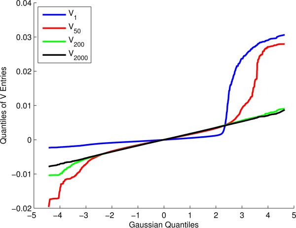
A second diagnostic was to examine the columns of V to check for Gaussianity related to the phenomenon mentioned in Section 4.1. Indeed, we find that some of the columns of V are quite non-Gaussian, as shown in Figure 12. However, this phenomenon is localized to only the columns of V corresponding to the very largest λ_i. Applying the unaltered EigenPrism procedure could cause two problems. First, if the the first columns of V are not Haar-distributed, T₂ could be biased and/or higher-variance than our theory accounts for. Second, recalling the interpretation of EigenPrism as a weighted regression of $z_i^2$ on λ_i, the fact that the problematic eigenvectors correspond to the largest eigenvalues means that they have high leverage, which exacerbates any unwanted bias or variance they create. Luckily, both problems can be remedied by running the EigenPrism SNR-estimation procedure (with Σ = I_p after standardizing the columns of X) with the added constraint to the optimization program in Equation (2.8) that the first entries of w are equal to zero. Explicitly, as the non-Gaussianity of the columns of V appears to dissipate after around the 100^th column, we set w₁ = ··· = w₁₀₀ = 0. The choice of 100 is somewhat subjective, but we tried other values and obtained very similar results. Because the resulting weights still obey the original constraints, the estimator of ${\Vert \beta \Vert }_2^2$ remains unbiased and motivated the variance upper-bounds remain valid. Although by the diagnostics from Section 4.1, this adjustment has the added advantage of making the entire EigenPrism procedure completely independent of the first 100 rows of U. It has been shown that the first rows of U are strongly related to the population structure of the sample (for example, the first two principal components correspond closely with subjects’ geographic origin), so constraining the first weights to be zero has the added effect of controlling for population structure (Price et al., 2006). As a final note, by subtracting off the means of each column of X, we reduced X's rank by one, resulting in λ_n = 0. As this is not actually reflective of the distribution of X, we also force w_n = 0 so that the last column of V and last row of U do not contribute to our estimate or inference.

Figure 12.

Distribution of the entries of some eigenvectors of the NFBC1966 design matrix.

Encouraged by the simulation results from Table 2, we proceeded to generate EigenPrism CIs for the SNRs of the 9 traits analyzed in Sabatti et al. (2009), as well as height (these 10 traits were also analyzed in Kang et al. (2010)). For each trait, transformation and subject exclusion was performed before computing SNR, following closely the procedures used in Sabatti et al. (2009); Kang et al. (2010) (see Appendix I for details). Lastly, all non-height phenotype values were adjusted for sex, pregnancy status, and oral contraceptive use, while height was only adjusted for sex. Table 3 gives the point estimate and 95% CI for the SNR of each phenotype, as well as the number of subjects used. Recall that these are CIs for the fraction of variance explained by the linear model consisting of the given array of SNPs. Still, these CIs generally agree quite well with heritability estimates in the literature (Kang et al., 2010). For instance, (Kang et al., 2010, Supplementary Information) reports two “pseudo-heritability” estimates of 73.8% and 62.5% for height, and 27.9% and 24.2% for BMI, on the same data set. This is somewhat remarkable given that they use a completely different statistical procedure with different assumptions. In particular, while other works in the heritability literature tend to treat β as random, EigenPrism was motivated by a simple model with β fixed and the rows of X random. We find this model more realistic, as true genetic effects are not in fact random, but fixed. One could argue the difference is not too important as long as the genetic effects are approximately distributed as the random effects model chosen, but such an assumption is impossible to verify in practice, as the true effects are never observed. EigenPrism's assumptions, on the other hand, are all on the design matrix, which is fully observed, leading to checks and diagnostics that can be performed to ensure the procedure will generate reasonable CIs.

Table 3.

CIs for heritability estimates for each of the 10 continuous phenotypes considered, along with the number of samples used for each.

Phenotype Name	# Samples	SNR 95% CI (%)	Point Estimate (%)
Triglycerides	4644	[3.1, 29.3]	16.2
HDL cholesterol	4700	[17.1, 42.9]	30.0
LDL cholesterol	4682	[27.7, 53.6]	40.7
C-reactive protein	5290	[5.6, 28.8]	17.2
Glucose	4895	[4.0, 28.9]	16.5
Insulin	4867	[0.0, 21.5]	9.0
BMI	5122	[8.9, 32.8]	20.9
Systolic blood pressure	5280	[7.8, 31.0]	19.4
Diastolic blood pressure	5271	[7.4, 30.7]	19.0
Height	5306	[46.0, 69.1]	57.6

6 Discussion

We have presented a framework for performing inference on the ${\ell }_2$-norm of the coefficient vector in a linear regression model. Although the resulting confidence intervals are asymptotic, we show in extensive simulations that they achieve nominal coverage in finite samples, without making any assumption on the structure or sparsity of the coefficient vector, or requiring knowledge of σ². In simulations, we are able to relax the restrictive assumptions on the distribution of the design matrix and gain an understanding of when our procedure is not appropriate. Applying this framework to performing inference on ${\ell }_2$ regression error, noise level, and genetic signal-to-noise ratio, we develop new procedures in all three that are able to construct accurate CIs in situations not previously addressed in the literature.

This work leaves open numerous avenues for further study. We briefly introduced a 2-step procedure that provided substantially shorter CIs than the EigenPrism procedure, but had less-consistent coverage. If we could better understand that procedure or come up with diagnostics for when it would undercover, we could improve on the EigenPrism procedure. We also explored in simulation a number of model failures that our procedure was robust (or not) to, but further study could provide theoretical guarantees on the coverage of the EigenPrism procedure for a broader class of random design models. Section 4.1 also briefly alluded to improved robustness in a random effects framework, which we have not explored further here. Finally, although in this work we consider a statistic that is linear in the $z_i^2$, the framework and ideas of this work are not intimately tied to this restriction, and there may exist statistics that are nonlinear functions of the $z_i^2$ that give improved performance.

References

- Abecasis GR, Auton A, Brooks LD, DePristo M. a., Durbin RM, Handsaker RE, Kang HM, Marth GT, McVean G. a. An integrated map of genetic variation from 1,092 human genomes. Nature. 2012;491:56–65. doi: 10.1038/nature11632. URL http://www.pubmedcentral.nih.gov/articlerender.fcgi?artid=3498066&tool=pmcentrez&rendertype=abstract. [DOI] [PMC free article] [PubMed] [Google Scholar]
- Bai ZD, Miao BQ, Pan GM. On asymptotics of eigenvectors of large sample covariance matrix. Ann. Probab. 2007;35:1532–1572. URL http://dx.doi.org/10.1214/009117906000001079. [Google Scholar]
- Bayati M, Erdogdu M, Montanari A. Estimating lasso risk and noise level. Advances in Neural Information Processing Systems. 2013:1–9. URL http://papers.nips.cc/paper/4948-estimating-lasso-risk-and-noise-level.
- Benjamini Y, Yu B. The shuffle estimator for explainable variance in fmri experiments. Ann. Appl. Stat. 2013;7:2007–2033. URL http://dx.doi.org/10.1214/13-AOAS681. [Google Scholar]
- Berk R, Brown L, Buja A, Zhang K, Zhao L. Valid post-selection inference. Ann. Statist. 2013;41:802–837. URL http://dx.doi.org/10.1214/12-AOS1077. [Google Scholar]
- Bonnet A, Gassiat E, Lévy-Leduc C. Heritability estimation in high dimensional linear mixed models. arXiv preprint arXiv. 2014;1404.3397. [Google Scholar]
- Candès E, Romberg J, Tao T. Robust uncertainty principles: exact signal reconstruction from highly incomplete frequency information. Information Theory, IEEE Transactions on. 2006;52:489–509. [Google Scholar]
- Dicker LH. Variance estimation in high-dimensional linear models. Biometrika. 2014;101:269–284. URL http://biomet.oxfordjournals.org/content/101/2/269.abstract. [Google Scholar]
- Fan J, Guo S, Hao N. Variance estimation using refitted cross-validation in ultrahigh dimensional regression. Journal of the Royal Statistical Society. Series B. 2012:37–65. doi: 10.1111/j.1467-9868.2011.01005.x. URL http://onlinelibrary.wiley.com/ doi/10.1111/j.1467-9868.2011.01005.x/full. [DOI] [PMC free article] [PubMed]
- van de Geer S, Bhlmann P, Ritov Y, Dezeure R. On asymptotically optimal confidence regions and tests for high-dimensional models. Ann. Statist. 2014;42:1166–1202. URL http://dx.doi.org/10.1214/14-AOS1221. [Google Scholar]
- Giraud C, Huet S, Verzelen N. High-dimensional regression with unknown variance. Statist. Sci. 2012;27:500–518. URL http://dx.doi.org/10.1214/12-STS398. [Google Scholar]
- Golan D, Rosset S. Accurate estimation of heritability in genome wide studies using random effects models. Bioinformatics (Oxford, England) 2011;27:i317–23. doi: 10.1093/bioinformatics/btr219. URL http://www.pubmedcentral.nih.gov/articlerender.fcgi?artid=3117387&tool=pmcentrez&rendertype=abstract. [DOI] [PMC free article] [PubMed] [Google Scholar]
- Grant M, Boyd S. Graph implementations for nonsmooth convex programs. In Recent Advances in Learning and Control. In: Blondel V, Boyd S, Kimura H, editors. Lecture Notes in Control and Information Sciences. Springer-Verlag Limited; 2008. pp. 95–110. [Google Scholar]
- Grant M, Boyd S. {CVX}: Matlab Software for Disciplined Convex Programming, version 2.1. 2014 url{ http://cvxr.com/cvx}.
- Järvelin M-R, Sovio U, King V, Lauren L, Xu B, McCarthy MI, Hartikainen A-L, Laitinen J, Zitting P, Rantakallio P, Elliott P. Early life factors and blood pressure at age 31 years in the 1966 northern finland birth cohort. Hypertension. 2004;44:838–846. doi: 10.1161/01.HYP.0000148304.33869.ee. URL http://hyper.ahajournals.org/content/44/6/838.abstract. [DOI] [PubMed] [Google Scholar]
- Javanmard A, Montanari A. Confidence intervals and hypothesis testing for high-dimensional regression. arXiv preprint arXiv. 2014;1306.3171 [Google Scholar]
- Kang HM, Sul JH, Service SK, Zaitlen NA, Kong S.-y., Freimer NB, Sabatti C, Eskin E. Variance component model to account for sample structure in genome-wide association studies. Nature genetics. 2010;42:348–354. doi: 10.1038/ng.548. [DOI] [PMC free article] [PubMed] [Google Scholar]
- Kang HM, Zaitlen NA, Wade CM, Kirby A, Heckerman D, Daly MJ, Eskin E. Efficient control of population structure in model organism association mapping. Genetics. 2008;178:1709–1723. doi: 10.1534/genetics.107.080101. URL http://www.genetics.org/content/178/3/1709.abstract. [DOI] [PMC free article] [PubMed] [Google Scholar]
- Knight K, Fu W. Asymptotics for lasso-type estimators. The Annals of Statistics. 2000;28:1356–1378. URL http://www.jstor.org/stable/2674097. [Google Scholar]
- Lee J, Sun D, Sun Y, Taylor J. Exact post-selection inference, with application to the lasso. arXiv preprint arXiv. 2015;1311.6238 [Google Scholar]
- Lockhart R, Taylor J, Tibshirani RJ, Tibshirani R. A significance test for the lasso. Ann. Statist. 2014;42:413–468. doi: 10.1214/13-AOS1175. URL http://dx.doi.org/10.1214/13-AOS1175. [DOI] [PMC free article] [PubMed] [Google Scholar]
- Manolio TA, Collins FS, Cox NJ, Goldstein DB, Hindorff LA, Hunter DJ, McCarthy MI, Ramos EM, Cardon LR, Chakravarti A. Finding the missing heritability of complex diseases. Nature. 2009;461:747–753. doi: 10.1038/nature08494. [DOI] [PMC free article] [PubMed] [Google Scholar]
- Marčenko V, Pastur L. Distribution of eigenvalues for some sets of random matrices. Sbornik: Mathematics. 1967;457 URL http://www.turpion.org/php/full/infoFT.phtml?journal_id=sm&paper_id=1994. [Google Scholar]
- Owen A. Quasi-regression for heritability. 2012:1–13. URL http://statweb.stanford.edu/~owen/reports/herit.pdf.
- Owen A. 2014. personal communication.
- Price AL, Patterson NJ, Plenge RM, Weinblatt ME, Shadick NA, Reich D. Principal components analysis corrects for stratification in genome-wide association studies. Nature genetics. 2006;38:904–909. doi: 10.1038/ng1847. [DOI] [PubMed] [Google Scholar]
- Pritchard J. Are rare variants responsible for susceptibility to complex diseases? The American Journal of Human Genetics. 2001:124–137. doi: 10.1086/321272. URL http://www.sciencedirect.com/science/article/pii/S0002929707614529. [DOI] [PMC free article] [PubMed]
- Sabatti C, Service SK, Hartikainen A-L, Pouta A, Ripatti S, Brodsky J, Jones CG, Zaitlen NA, Varilo T, Kaakinen M, Sovio U, Ruokonen A, Laitinen J, Jakkula E, Coin L, Hoggart C, Collins A, Turunen H, Gabriel S, Elliot P, McCarthy MI, Daly MJ, Jrvelin M-R, Freimer NB, Peltonen L. Genome-wide association analysis of metabolic traits in a birth cohort from a founder population. Nature genetics. 2009;41:35–46. doi: 10.1038/ng.271. [DOI] [PMC free article] [PubMed] [Google Scholar]
- Silventoinen K, Sammalisto S, Perola M, Boomsma DI, Cornes BK, Davis C, Dunkel L, de Lange M, Harris JR, Hjelmborg JVB, Luciano M, Martin NG, Mortensen J, Nisticò L, Pedersen NL, Skytthe A, Spector TD, Stazi MA, Willemsen G, Kaprio J. Heritability of Adult Body Height: A Comparative Study of Twin Cohorts in Eight Countries. Twin Research and Human Genetics. 2003;6:399–408. doi: 10.1375/136905203770326402. URL http://journals.cambridge.org/article_S1369052300004001. [DOI] [PubMed] [Google Scholar]
- Städler N, Bühlmann P, van de Geer S. 1-Penalization for Mixture Regression Models. Test. 2010;19:209–256. URL http://link.springer.com/10.1007/s11749-010-0197-z. [Google Scholar]
- Sun T, Zhang C-H. Scaled sparse linear regression. Biometrika. 2012;99:879–898. URL http://biomet.oxfordjournals.org/cgi/doi/10.1093/biomet/ass043. [Google Scholar]
- Taylor J, Lockhart R, Tibshirani R, Tibshirani R. Exact post-selection inference for forward stepwise and least angle regression. arXiv preprint arXiv. 2014;1401.3889 [Google Scholar]
- Tibshirani R. Regression shrinkage and selection via the lasso. Journal of the Royal Statistical Society. Series B. 1996;58:267–288. URL http://www.jstor.org/stable/10.2307/2346178. [Google Scholar]
- Visscher PM, Hill WG, Wray NR. Heritability in the genomics eraconcepts and misconceptions. Nature Reviews Genetics. 2008;9:255–266. doi: 10.1038/nrg2322. [DOI] [PubMed] [Google Scholar]
- Ward R. Compressed sensing with cross validation. Information Theory, IEEE Transactions on. 2009;55:5773–5782. URL http://ieeexplore.ieee.org/xpls/abs_all.jsp?arnumber=5319752. [Google Scholar]
- Weedon MN, Lango H, Lindgren CM, Wallace C, Evans DM, Mangino M, Freathy RM, Perry JRB, Stevens S, Hall AS. Genome-wide association analysis identifies 20 loci that influence adult height. Nature genetics. 2008;40:575–583. doi: 10.1038/ng.121. [DOI] [PMC free article] [PubMed] [Google Scholar]
- Yang J, Benyamin B, McEvoy BP, Gordon S, Henders AK, Nyholt DR, Madden PA, Heath AC, Martin NG, Montgomery GW. Common SNPs explain a large proportion of the heritability for human height. Nature genetics. 2010;42:565–569. doi: 10.1038/ng.608. Others. [DOI] [PMC free article] [PubMed] [Google Scholar]
- Zhang C-H, Zhang SS. Confidence intervals for low dimensional parameters in high dimensional linear models. Journal of the Royal Statistical Society: Series B (Statistical Methodology) 2014;76:217–242. URL http://dx.doi.org/10.1111/rssb.12026. [Google Scholar]
Associated Data
This section collects any data citations, data availability statements, or supplementary materials included in this article.