Abstract
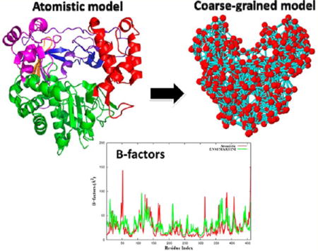
In this article, we present a hybrid ENM/MARTINI coarse-grained model and examine the impact of reduced chemical detail on both static and dynamic properties by comparing against explicit atomistic simulations. This methodology complements the advanced molecular characterization and dynamics of proteins for medical and bioengineering applications by developing a fundamental understanding of how the motion and molecular characteristics of proteins, viruses, their precursors, and their interactions with the environment govern their behavior in different populations. As an example, we explore the dynamics of RNA-dependent RNA polymerases (RdRPs) from the following viruses: poliovirus, Coxsackie virus B3, human rhinovirus 16, and foot-and-mouth-disease virus. The hybrid coarse-grained model allows the microsecond time scales of interest for biological functions to be explored. Additionally, the ENM/MARTINI model captures the main features obtained from atomistic MD simulations for each of the RdRPs studied herein, including the higher flexibility of the pinky finger and thumb regions, as well as collective motions that might contribute significantly to the conformational transition between the open and closed states.
Graphical abstract
INTRODUCTION
Currently, it is widely accepted that a folded protein should be represented as an ensemble of numerous conformations fluctuating in the neighborhood of its native state.1,2 Thus, the structure–function relationship should also be extended to include protein dynamics.2 With the realization that protein motions play important roles during biological processes, the study of protein dynamics has received a large amount of attention during recent years.1–4 However, it is not feasible to take detailed “snapshots” of every atom moving within a protein experimentally. Even though nuclear magnetic resonance (NMR) spectroscopy has emerged to study protein dynamics, the ability of NMR spectroscopy is still limited by protein size. Because of the increase in computational power and the significant improvement in energy functions, atomistic molecular dynamics (MD) simulations have become a complementary technique that is capable of providing detailed information about atomic motions in proteins as a function of time. Since the first MD simulation of a small protein performed in a vacuum with a total simulation time of 9.5 ps in 1977,1 the length of an atomistic MD simulation for a typical protein–solvent system currently extends to several hundred nanoseconds.
Despite the enormous progress made in the development of computer algorithms and processor speed during the past 20 years, conventional atomistic MD simulations are still prohibitive for studying many biological processes, such as protein folding and enzyme catalysis,5,6 that occur in the range of microseconds to seconds. Thus, to extend the applicability of MD simulations to study biological processes occurring on longer time scales, it is necessary to use a simplified representation of protein–solvent systems, instead of an atomic-detail description. Thus, a variety of coarse-grained (CG) models have been developed to allow MD simulations to study many biological processes occurring on longer time scales by reducing the number of degrees of freedom of the protein–solvent system and increasing the integration time step by at least a factor of 10 when compared to those used in atomistic MD simulations.7,8
Two CG models are of main interest in this work. First, the elastic network model (ENM) has been successfully used to study the slow motions of proteins. The ENM arises from the elastic theory of random polymer networks9 and was extended to study protein dynamics by using a normal-mode analysis (NMA) and simplified harmonic potentials.10,11 The second model, the MARTINI coarse-grained force field, was developed by Marrink and co-workers12 for modeling lipids and surfactants. The current MARTINI model (MARTINI v2.1) has been extended to simulate protein systems13 and has also been used to study the interactions between proteins and the lipid bilayer.14 In the latter case, the native structure of a protein is represented using an ENM. In this approach, the elastic network in the protein is constructed by means of backbone beads (one backbone bead per residue is located at the Cα atom position), and any two backbone beads within a distance of 7 Å are connected by a spring with a force constant of 1000 kJ·mol−1·nm−2. Periole and co-workers15 systematically investigated the optimum force constant for the restraint applied in the elastic network with different cutoff distances, and recommended that the spring constant should be in the range of 500–1000 kJ·mol−1·nm−2 when the cutoff distance in the elastic network is chosen in the range of 8–10 Å. The combination of the MARTINI model and the elastic network model was named ELNEDIN by the authors.15
In this work, instead of using a fixed force constant for the restraint in the elastic network, we elected to introduce a set of individual force constants that were applied to each pair of nonsequentially connected backbone beads. Individual force constants have also been used in other works16–18 and have been shown to be effective. The preliminary force constants and the equilibrium distance (within a cutoff value of 12 Å) between backbone beads were obtained from the trajectory of a short atomistic MD simulation (2 ns) of the protein using the Boltzmann inversion method.19 The implementation of the ENM over MARTINI, that is, imposing additional CG force constants obtained from short atomistic MD simulations preserved at the mesoscale, maintains the structural “scalfold” biased toward a reference structure. Additionally, it allows the most important dynamic features captured from time-consuming atomistic MD simulations to be preserved at the mesoscale. A similar behavior has been found in other works.12–14 In addition, the use of individual force constants for the elastic network provides a method (termed ENM/MARTINI here) that not only reaches microsecond time scales with good accuracy when compared against atomistic simulations but also reveals the different dynamics of single mutations within a protein at the mesoscale level. This last topic is outside the scope of the present work and will be addressed in a forthcoming publication.
Here, we apply the hybrid ENM/MARTINI coarse-grained model to study the dynamics of four different RNA-dependent RNA polymerases from poliovirus (PV), Coxsackie virus B3 (CVB3), human rhinovirus 16 (HRV16), and foot-and-mouth-disease virus (FMDV). An RNA-dependent RNA polymerase (RdRP) is an enzyme that catalyzes the replication of RNA from an RNA template. The crystal structures of the RdRPs from PV,20 CVB3,21 HRV16, 22 and FMDV23 studied in this work have an overall similar topology (see Figure 1). The structure of an RdRP resembles a cupped right hand and contains three subdomains: fingers, palm, and thumb.24 The structural description of the RdRp from poliovirus (PV) is given in ref 20 and summarized here for completeness. For poliovirus, which contains a prototypical RdRP, the fingers subdomain begins with a buried N terminus that is part of the index finger (residues 1–68). The pinky finger has two segments, residues 96–149, which proceed to the ring finger (residues 150–179), and residues 180–190, which are succeeded by residues of the palm. The middle finger (residues 269–285) is followed by residues of the palm.
Figure 1.
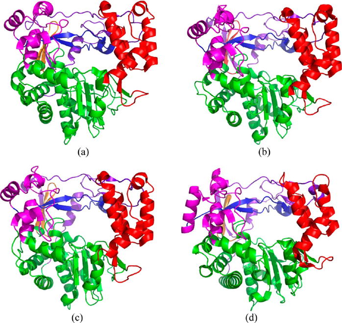
Ribbon representations of the crystal structures of the RdRPs from (a) PV, (b) CVB3, (c) HRV16, and (d) FMDV. Purple, magenta, blue, orange, green, and red colors represent the index finger, pinky finger, ring finger, middle finger, palm, and thumb subdomains, respectively.
A common property of RdRPs is the presence of several conserved structural motifs (A–G). The fingers subdomain subdomain contains motifs F (residues 153–178) and G (residues 113–120). The palm contains the remaining five motifs A (residues 229–240), B (residues 293–312), C (residues 322–335), D (residues 338–362), and E (residues 363–380). Finally, the thumb is composed of the C-terminal residues 381–461, which form a bundle of α-helices. The strong interactions between fingertips and thumb result in a completely encircled active site, forming the entry/exit channel for template-primer RNA and NTP substrates.
In the following sections, we provide background information on the ENM and MARTINI force fields and simulation methods, discuss our model and systems, and finally describe conclusions about the behavior of our systems based on our simulations.
METHODS
Elastic Network Model
In the elastic network model (ENM),10,11 a folded protein is assumed to be a three-dimensional elastic network in which each amino acid residue is usually represented as a bead using the position of the Cα atom. Two beads are connected by a harmonic spring, described by a simplified harmonic potential function
| (1) |
Here, γ is the Hookean pairwise force constant representing the interaction between two residues in the folded protein; the element ΔRi of ΔR is the fluctuation vector of the ith residue; and Ģ is a symmetric matrix known as the Kirchhoff matrix
| (2) |
where Rcut is the cutoff distance giving the range of the interaction between two residues and Rij is the separation between the ith and jth residues.
MARTINI Coarse-Grained Model
The MARTINI12,13 coarse-grained representation of the 20 amino acids is presented in Figure 1 of ref 13 and summarized here. The coarse-grained model uses the four-to-one mapping method. Thus, four heavy atoms of an amino acid, except for an amino acid having a ringlike fragment, are grouped into a bead, with each bead representing an interaction site. For different ringlike fragments, the model uses different mappings with higher resolution (up to two-to-one mapping). The type of each interaction site is one of four different main types: polar (P), nonpolar (N), apolar (C), and charged (Q). In addition to the four main types, different subtypes are defined either by the hydrogen-bonding capacity (donor, acceptor, both, or none) or by the degree of polarity (increasing from 1 to 5). A detailed description of the interaction type for each amino acid is given in Table 1 of ref 13, and the interested reader is referred to this publication for further information.
ENM/MARTINI Coarse-Grained Model
In the hybrid model presented here, the MARTINI coarse-grained force field without any modification was used with additional harmonic restraints imposed on the nonsequentially connected centers of mass of the backbone beads within a predetermined distance (e.g., 12 Å). Thus, the main difference between the ENM/MARTINI and MARTINI models is the additional elastic restraint imposed on the backbone beads. The partial three-dimensional structure of the protein, represented only by the backbone beads, is then modeled as an elastic network, as shown in Figure 2. The harmonic restraint Vij between the ith and jth backbone beads (1 ≤ i < j ≤ N, j − i > 1, where N is the total number of residues of a protein) is given by
| (3) |
where Kij is the force constant and dij and are the instantaneous distance and the equilibrium distance, respectively, between the ith and jth backbone beads. The force constants Kij for the springs connecting the ith and jth backbone beads were individually obtained from the trajectory of a short atomistic MD simulation (2 ns) through the Boltzmann inversion technique. First, we assume that the motion of the centers of mass of the backbone atoms at the ith and jth residues can approximately be described by a simple harmonic potential in the short atomistic MD simulation. Second, the probability distribution Pij of the distance dij between the ith and jth centers of mass is calculated from atomistic MD simulations. Finally, the resulting probability distribution Pij is used to obtain the CG force constant Kij according to the relationship
| (4) |
where kB is the Boltzmann constant and T is the absolute temperature. Preliminary studies for the PV RdRP (Figure S1a of the Supporting Information) showed that the calculated force constants needed to be rescaled for the system to achieve proper flexibility. Several different scaling factors (e.g., ½, ¼, , , and ) were tested, and the rescaled force constants were applied in the ENM/MARTINI simulations of the four RdRPs studied in this work; see Figure S1 of the Supporting Information. From a comparison of B factors between the atomistic and coarse-grained models, we observed that the best scaling factors were in the range from to , and in this work we chose a scaling factor of . The necessity of a scaling factor comes from the known acceleration of the sampling of the phase space by the MARTINI model, which is a direct effect of the neglect of atomic degrees of freedom in the CG simulations. Similar conclusions have been drawn from the analysis of chain configurations in lipid bilayers and hydrocarbon chains, as mentioned in refs 12–14 and references therein.
Figure 2.
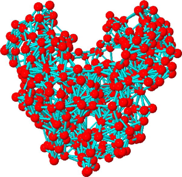
Elastic network representation of the backbone beads of the RdRP from PV. The red beads and cyan sticks represent the backbone and springs connecting backbone particles, respectively.
Atomistic MD Simulations
Long atomistic MD simulations for the RNA-dependent RNA polymerases from PV, CVB3, HRV16, and FMDV were previously performed.25 For completeness, we summarize the most important details here. The initial structures of the RdRPs were obtained from the X-ray structures found in the Protein Data Bank: PV (PDB entry 1RA6), CVB3 (PDB entry 3CDU), HRV16 (PDB entry 1XR7), and FMDV (PDB entry 1U09). The proteins were solvated in a truncated octahedral box of TIP3P water molecules,26 with a distance of at least 20 Å between the surface of each protein and the edge of the water box. MD simulations were carried out with the AMBER 10 molecular dynamics simulation package,27 and the AMBER 99 force field28 using SANDER for the initial minimizations and PMEMD for subsequent MD simulations. Each protein–solvent system was heated stepwise from 0 to 300 K with an increment of 50 K over a period of 10 ps at a constant volume, and this was followed by 200 ps of NVT simulation. Finally, NPT simulations were carried out at 300 K. The atomistic MD simulations used an integration time step of 1 fs, and the cutoff distance for the nonbonded interactions updated every 10 steps was 9 Å. The Berendsen thermostat29 for temperature coupling with a time constant of 0.05 ps was applied. The total length of the MD simulations carried out for the four protein–solvent systems was up to 50 ns each.
Coarse-Grained MD Simulations
The MARTINI and ENM/MARTINI simulations of the RdRPs from PV, CVB3, HRV16, and FMDV were performed with the GROMACS 4.0 molecular dynamics simulation package.30 The general topology files, parameter files, and scripts to generate topology files for the proteins were downloaded from the Web site for the MARTINI coarse-grained force field (http://md.chem.rug.nl/~marrink/coarsegrain). The proteins were solvated in a cubic box of 86 × 86 × 86 Å3 with coarse-grained water molecules (one coarse-grained water molecule corresponds to four water molecules). An energy minimization with a steepest-descent algorithm was performed for 2000 steps and was followed by heating the protein–solvent systems stepwise from 0 to 300 K at 50 K increments. The temperature (300 K) for NVT simulations followed by NPT simulations was kept constant using the Berendsen temperature-coupling algorithm29 with a time constant of 1.0 ps. Considering the elastic restraints being imposed, anisotropic pressure coupling was applied using the Berendsen algorithm with a time constant of 5.0 ps and a compressibility of 4.5 × 10⁻⁵ bar−1, under a pressure of 1 bar. Shifted potentials were used in the simulations, where the Lennard-Jones potential was shifted to zero from 0.9–1.2 nm and the electrostatic potential was shifted to zero from 0–1.2 nm. The integration time step of the simulations was set to 30 fs, and the total length of each run was approximately 1.2 μs. The drawings of the protein structures considered in this work were prepared with the VMD program.31
RESULTS AND DISCUSSION
Performance of MARTINI and ENM/MARTINI Coarse-Grained Models
To examine the performance of the coarse-grained models, the ENM/MARTINI and MARTINI simulations for PV were carried out. The root-mean-square deviations (RMSDs) and radii of gyration (RG) obtained for PV from the MARTINI and ENM/MARTINI simulations are plotted in Figure 3. The figure shows that both the MARTINI and ENM/MARTINI simulations were equilibrated within 0.1 μs. Thus, the interval of the first 0.1 μs was considered as an equilibration stage, and the subsequent production run was used for data analysis. During the equilibration stage, the RMSD of the MARTINI simulation significantly increased to about 5 Å whereas the RMSD of the ENM/MARTINI simulation did not exceed 3 Å. The ENM/MARTINI and MARTINI simulations of the other RdRPs (CVB3, HRV16, and FMDV) showed similar behavior (see Figure S2b–d, Supporting Information). Therefore, the additional harmonic restraint imposed on the centers of mass of the backbone beads using the hybrid approach, ENM/MARTINI, was able to sustain the native structure of the folded proteins during the simulations.
Figure 3.
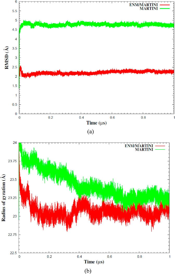
(a) RMSD curves and (b) radii of gyration of MARTINI (green) and ENM/MARTINI (red) simulations of the PV RdRP.
Use of the atomic displacement parameter, or B factor, defined as
| (5) |
is a simple method for analyzing the fluctuation of an atom about its average position in a protein. Here, Δri is the position fluctuation of the ith atom. The distribution of B factors along the amino acid sequence of a protein provides an indication of the protein’s flexibility and dynamics. Larger values of the B factor correspond to higher flexibility, and vice versa. In addition, analysis of the B factor can be used to test the quality of a coarse-grained simulation when compared with an atomistic MD simulation. Thus, the B factors of the α-carbon atoms for the RdRp from PV obtained from the ENM/MARTINI simulation and the MARTINI simulation are plotted in Figure 4. From Figure 4a, one can see that the flexibility of many amino acid residues was predicted well using the MARTINI simulation, but the quality of the predictions was improved by combining MARTINI with the elastic network model, as shown in Figure 4b.
Figure 4.
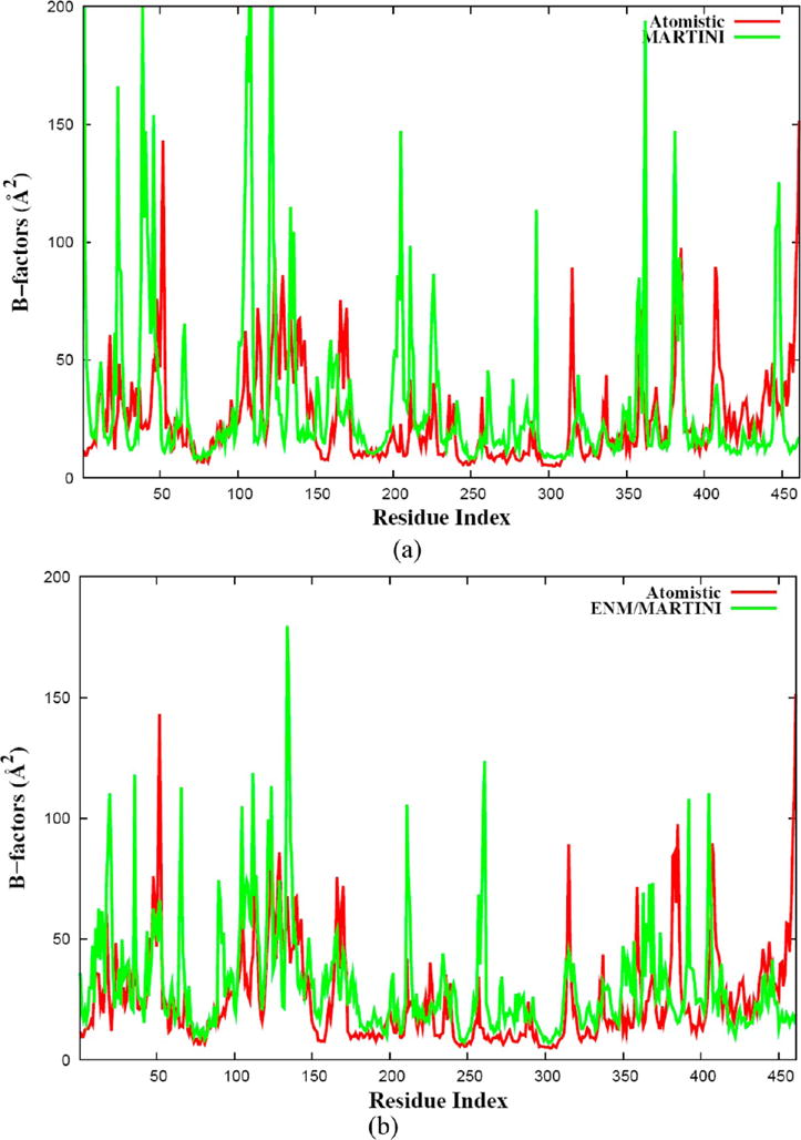
B factors of the PV RdRP obtained from (a) MARTINI and (b) ENM/MARTINI simulations over the last 700 ns. The coarse-grained results (green) were compared with the results of atomistic MD simulation (red) over the last 5 ns.
Global Dynamics of RdRps
The B factors of the other three RdRps from CVB3, HRV16, and FMDV were obtained from the ENM/MARTINI simulation, and we observed that the ENM/MARTINI simulation approximately predicted the regions with high flexibility or low flexibility as the atomistic MD simulations did; see Figure 5. Furthermore, the quality of the B factors could be improved by enhancing the sampling in the simulations, which will be discussed later in this section. Because the four RdRps (PV, CVB3, HRV16, and FMDV) share similar dynamic features, in what follows, we discuss the global dynamics of only the PV RdRp, as observed from the results for the B factors.
Figure 5.
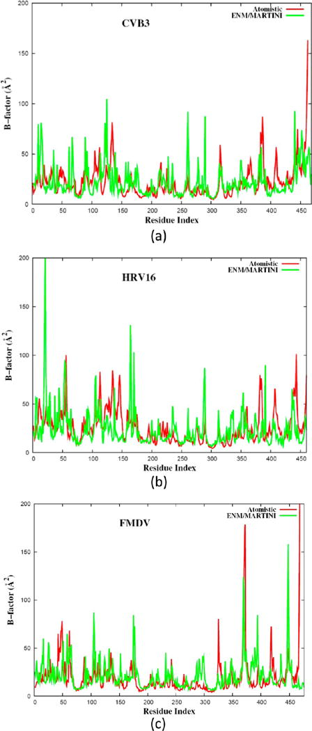
B factors of the RdRPs from (a) CVB3, (b) HRV16, and (c) FMDV obtained from ENM/MARTINI simulations (green) and from atomistic MD simulations (red).
The ENM/MARTINI simulation of the PV RdRp revealed that the fingers subdomain (blue color in Figure 1) is, in general, more flexible than the palm (green color in Figure 1) and thumb (red color in Figure 1) subdomains, and this observation was also found in atomistic MD simulation (see Figure 4b). In the ENM/MARTINI simulation, we found that the magnitude of the flexibility at some residues was overestimated and the high flexibility of the segment (residues 382–386) of the thumb was not observed. However, we were able to improve the results of our ENM/MARTINI simulation by enhancing the sampling of configurations, which we did by performing six independent ENM/MARTINI simulations of the PV RdRp using the same coarse-grained simulation protocol but different initial velocities. Thus, the six trajectories (1.2 μs each) allowed us to study the events on a ~7.2-μs time scale (Figure 4Sa, Supporting Information). The average results for the B factors over the six trajectories are plotted in Figure 6, where one can see an improvement of the B factors in comparison with those from a single simulation (Figure 4b).
Figure 6.
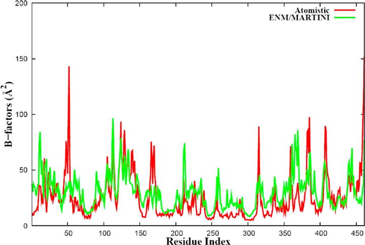
B factors of the PV RdRP obtained from the average of six independent ENM/MARTINI simulations (green) and from atomistic MD simulation (red).
The improved results for the B factors (Figure 6) demonstrate that the ENM/MARTINI simulation is able to capture the global dynamic features obtained from atomistic MD simulations. We summarize some flexible regions detected by the ENM/MARTINI simulation as follows:
Two segments (residues 11–33 and 48–66) of the index finger, mainly containing random coils and exposed to solvent, are expected to be flexible. One should note, however, that the magnitude of the high-flexibility residues is sensitive to the time window chosen for analysis in the atomistic MD simulation (data not shown), so it is acceptable that the flexibility of residues 48–52 is underestimated in the ENM/MARTINI simulation. The segment consisting of residues 113–137, containing motif G (residues 113–120), sits on the top of the pinky finger, and it exhibits high flexibility.20 Motif F (residues 153–178) of the ring finger, serving as the binding site of the incoming NTP, displays a certain flexibility in the ENM/MARTINI simulation.
Residues 211–213 and 257–261 of the palm still show high flexibility in the enhanced ENM/MARTINI simulations. The ENM/MARTINI simulation also detected the flexible segment containing residues 314–317 that belongs to a loop between motifs B (residues 293–312) and C (residues 322–335). The function of this flexible loop is not clear. The ENM/MARTINI simulation revealed that motifs A (residues 229–240), B, and C are less flexible than motif D (residues 338–362), which is an important element affecting the rate of catalysis.32 Thus, knowledge of the motif D dynamics is becoming an important key to understanding RdRp fidelity.
Finally, the three highly flexible segments of the thumb were found at the residues 381–387, 403–412, and 436–449. The first segment is a loop between two β-sheets; the second segment contains a short β-sheet, a short loop, and part of a long helix; and the last segment consists of a hydrogen-bonded turn, a short α-helix, and a coil.
Open and Closed States of RdRps
Knowledge of the open and closed forms of an enzyme and the conformation changes between the two could help to elucidate the mechanism of enzyme catalysis. The open conformation is needed for the RNA substrate to enter and then bind to the enzyme or for products to be released from the enzyme, whereas the closed conformation is required to form the active configuration for catalysis.
The radius of gyration is able to serve as a measure of the size of a globular protein in the course of a simulation, and the size of the globular protein can indicate whether the protein is in the closed or open conformation. The radii of gyration of the four RNA-dependent RNA polymerases (PV, CVB3, HRV16, and FMDV) obtained from the ENM/MARTINI simulations showed that the four proteins expanded and then contracted during the equilibration stage of the simulations (see Figures S3 and S4 in the Supporting Information). After the systems had equilibrated, the radii of gyration of the four polymerases achieved equilibrated values of 23.1, 23.2, 23.4, and 23.4 Å for PV, CVB3, HRV16, and FMDV, respectively. The radii of gyration of the crystal structures of the four proteins were measured to be about 22.6, 22.7, 23.0, and 23.0 Å for PV, CVB3, HRV16, and FMDV, respectively, so the radii of gyration of the four proteins were increased by about 2% in the ENM/MARTINI simulations. Therefore, the conformations sampled in the ENM/MARTINI simulations correspond to the open states, whereas the crystal structures correspond to the closed states.
To observe the open-to-closed conformation transition in the ENM/MARTINI simulation, we took an average structure of each ENM/MARTINI trajectory and superimposed it on the corresponding crystal structure (Figure 7), from which we found a similar pattern of conformational change between the closed and open states among the four proteins. To display the transition more clearly, the segments at the top of the pinky finger and thumb are highlighted in Figure 8, and we found that the open-to-closed conformation transition is characterized by the movement of the fingers and thumb toward the RNA entry channel. This observation is consistent with the results from our previous atomistic MD simulation of the PV RdRp.25
Figure 7.
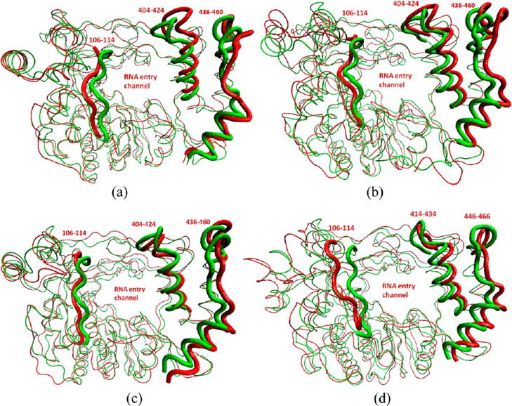
Open (red) conformations of the RdRPs from (a) PV, (b) CVB3, (c) HRV16, and (d) FMDV obtained from ENM/MARTINI simulations. The crystal structures of the four RdRPs are represented in green. Some segments are highlighted for clarity.
Figure 8.
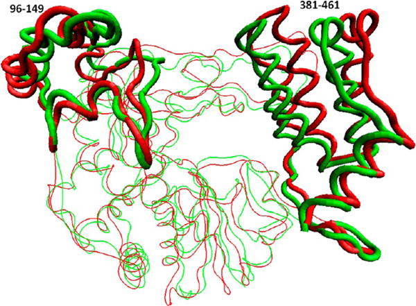
Open (red) and closed (green) conformations of the PV RdRP obtained from six independent ENM/MARTINI simulations. A segment of the pinky finger (residues 96–149) and the Thumb (residues 381–461) are highlighted.
Coupled Motions in the PV RdRP from Open to Closed States
Although B factors provide information about the magnitude of a protein residue’s fluctuations, they do not provide information about coupled motions of residues. As the four RdRPs studied in this work share similar patterns, we analyzed the coupled motions of different segments from the PV RdRP. (Results for the other three RdRPs can be found in the Supporting Information.) In this work, we used the average-distance matrix over time (see Figure 9) to identify residues with coupled motions. The minimum-distance matrix is a matrix that shows the smallest distance between two residues in a protein. For example, residues 26–38, which belong to the index finger at the back of the thumb, kept a close distance with residues 400–410 of the thumb during the ENM/MARTINI simulation, which promotes the coupled motion between them, as seen in the left top corner of Figure 9 and in Figure 10a. Although residues 26–38 had a greater separation from residues 435–440 of the thumb during the course of the simulation, their coupled motion was still observed (Figures 9 and 10b). Thus, the coupled motions of the three segments consisting of residues 26–38, 400–410, and 435–440 facilitate the collective motion of the thumb subdomain. The two segments consisting of residues 110–118 and 126–134 of the pinky finger sit at the top of the fingers, and the coupled motion between them (Figures 9 and 10c) is ascribed to their preserved close distance. This distance thus represents their interactions during the simulation. Similarly, the coupled motion of residues 110–118 and 126–134 supports the collective motion of the fingers at the top of the polymerase. Therefore, the open-to-closed conformation transition, characterized by the collective motions of the fingers and thumb toward the RNA entry channel, was observed in our ENM/MARTINI simulation. These data therefore confirm the result of dynamic cross-correlation maps calculated from atomistic MD simulations.25
Figure 9.
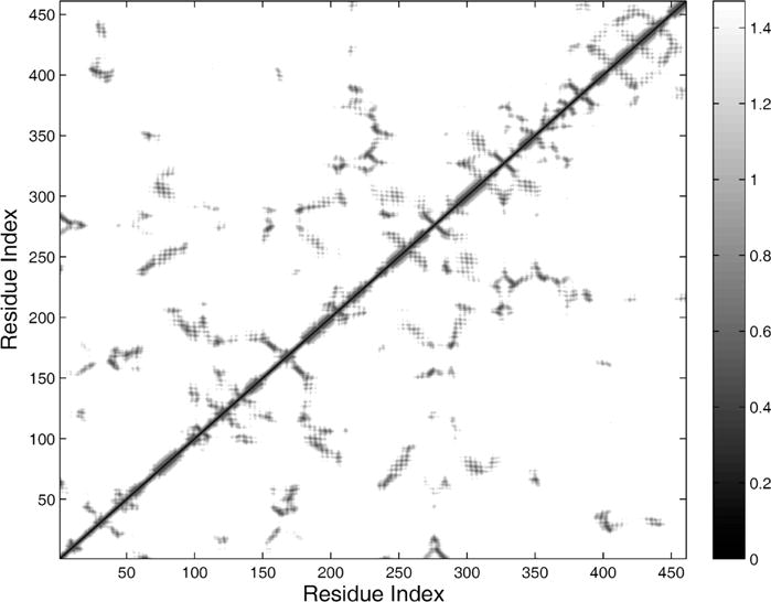
Minimum-distance matrix of the PV RdRP obtained from ENM/MARTINI simulations over the last 700 ns.
Figure 10.
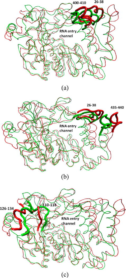
Open (red) and closed (green) conformations of the PV RdRP obtained from six independent ENM/MARTINI simulations and observed coupled motions (a) between the segments 26–38 and 400–410), (b) between the segments 26–38 and 435–440, and (c) between the segments 126–134 and 110–118.
CONCLUSIONS
A hybrid ENM/MARTINI coarse-grained model with a set of individual force constants determined from short atomistic molecular dynamic simulations has been presented in this work to explore the dynamics of four different RNA-dependent RNA polymerases (RdRPs) from poliovirus, Coxsackievirus B3, human rhinovirus 16, and foot-and-mouth-disease virus. The results of the ENM/MARTINI simulations described herein are encouraging and show that the hybrid coarse-grained force field not only is able to capture the main features obtained from atomistic MD simulations but should also permit exploration of protein motion on a microsecond time scale.
The coarse-grained MD simulations performed for each of the RdRPs examined in this work revealed that (1) in general, the pinky finger and the thumb at the top of each polymerase have higher flexibility than other regions; (2) the closing of the RNA entry channel is characterized by the motions of the finger and thumb subdomains, that is, the movement of the fingers and thumb toward the RNA entry channel; and (3) the ENM/MARTINI simulations are able to capture collective motions that might contribute significantly to the conformational transition between the open and closed states. Finally, our study supports the likelihood that the combination of an elastic network model and the MARTINI coarse-grained force field might be a promising method for overcoming some limitations of the MARTINI model.
Supplementary Material
Acknowledgments
This work was supported in part by the NIH/NIAID grant AI45818 and the MRI and Huck Institutes at Penn State. This research was also supported in part by the National Science Foundation through TeraGrid resources provided by the Pittsburgh Supercomputing Center, Grant MCB080068N. Additionally, we acknowledge Dr. Ping Lin, of the Materials Simulation Center, and the computing resources from the ITS-HPC group at Penn State.
Footnotes
Supporting Information
B factors obtained from the ENM/MARTINI simulations with different elastic restraints (Figure S1) and RMSD curves and radii of gyration for different polymerases (Figure S2–S4). This material is available free of charge via the Internet at http://pubs.acs.org.
Notes
The authors declare no competing financial interest.
References
- 1.McCammon JA, Gelin BR, Karplus M. Nature. 1977;267:585–590. doi: 10.1038/267585a0. [DOI] [PubMed] [Google Scholar]
- 2.Henzler-Wildman KA, Kern D. Nature. 2007;450:964–972. doi: 10.1038/nature06522. [DOI] [PubMed] [Google Scholar]
- 3.Karplus M, McCammon JA. Nat Struct Biol. 2002;9:646–652. doi: 10.1038/nsb0902-646. [DOI] [PubMed] [Google Scholar]
- 4.Karplus M, Kuriyan J. Proc Natl Acad Sci U S A. 2005;102:6679–6685. doi: 10.1073/pnas.0408930102. [DOI] [PMC free article] [PubMed] [Google Scholar]
- 5.Dill KA, Ozkan SB, Weikl TR, Chodera JD, Voelz VA. Curr Opin Struct Biol. 2007;17:342–346. doi: 10.1016/j.sbi.2007.06.001. [DOI] [PubMed] [Google Scholar]
- 6.Henzler-Wildman KA, Lei M, Thai V, Kerns SJ, Karplus M, Kern D. Nature. 2007;450:913–916. doi: 10.1038/nature06407. [DOI] [PubMed] [Google Scholar]
- 7.Voth G. Coarse-Graining of Condensed Phase and Biomolecular Systems. CRC Press; Boca Raton, FL: p. 2008. [Google Scholar]
- 8.Tozzini V. Curr Opin Struct Biol. 2005;15:144–150. doi: 10.1016/j.sbi.2005.02.005. [DOI] [PubMed] [Google Scholar]
- 9.Kloczkowski A, Mark JE. Macromolecules. 1989;22:1423–1432. [Google Scholar]
- 10.Tirion MM. Phys Rev Lett. 1996;77:1905–1908. doi: 10.1103/PhysRevLett.77.1905. [DOI] [PubMed] [Google Scholar]
- 11.Haliloglu T, Bahar I, Erman B. Phys Rev Lett. 1997;79:3090–3093. [Google Scholar]
- 12.Marrink SJ, Risselada HJ, Yefimov S, Tieleman DP, de Vries AH. J Phys Chem B. 2007;111:7812–7824. doi: 10.1021/jp071097f. [DOI] [PubMed] [Google Scholar]
- 13.Monticelli L, Kandasamy SK, Periole X, Larson RG, Tieleman DP, Marrink SJ. J Chem Theory Comput. 2008;4:819–834. doi: 10.1021/ct700324x. [DOI] [PubMed] [Google Scholar]
- 14.Balali-Mood K, Bond PJ, Sansom MSP. Biochemistry. 2009;48:2135–2145. doi: 10.1021/bi8017398. [DOI] [PubMed] [Google Scholar]
- 15.Periole X, Cavalli M, Marrink SJ, Ceruso MA. J Chem Theory Comput. 2009;5:2531–2543. doi: 10.1021/ct9002114. [DOI] [PubMed] [Google Scholar]
- 16.Kurkcuoglu O, Turgut OT, Cansu S, Jernigan RL, Doruker P. Biophys J. 2009;97:1178–1187. doi: 10.1016/j.bpj.2009.06.009. [DOI] [PMC free article] [PubMed] [Google Scholar]
- 17.Lyman E, Pfaendtner J, Voth GA. Biophys J. 2008;95:4183–4192. doi: 10.1529/biophysj.108.139733. [DOI] [PMC free article] [PubMed] [Google Scholar]
- 18.Ayton GS, Lyman E, Voth GA. Faraday Discuss. 2010;144:347–357. doi: 10.1039/b901996k. [DOI] [PMC free article] [PubMed] [Google Scholar]
- 19.Reith D, Pÿtz M, Mÿller-Plathe F. J Comput Chem. 2003;24:1624–1636. doi: 10.1002/jcc.10307. [DOI] [PubMed] [Google Scholar]
- 20.Thompson AA, Peersen OB. EMBO J. 2004;23:3462–3471. doi: 10.1038/sj.emboj.7600357. [DOI] [PMC free article] [PubMed] [Google Scholar]
- 21.Gruez A, Selisko B, Roberts M, Bricogne G, Bussetta C, Jabafi I, Coutard B, De Palma AM, Neyts J, Canard B. J Virol. 2008;82:9577–9590. doi: 10.1128/JVI.00631-08. [DOI] [PMC free article] [PubMed] [Google Scholar]
- 22.Love RA, Maegley KA, Yu X, Ferre RA, Lingardo LK, Diehl W, Parge HE, Dragovich PS, Fuhrman SA. Structure. 2004;12:1533–1544. doi: 10.1016/j.str.2004.05.024. [DOI] [PubMed] [Google Scholar]
- 23.Ferrer-Orta C, Arias A, Perez-Luque R, Escarm’s C, Domingo E, Verdaguer N. J Biol Chem. 2004;279:47212–47221. doi: 10.1074/jbc.M405465200. [DOI] [PubMed] [Google Scholar]
- 24.Hansen JL, Long AM, Schultz SC. Structure. 1997;5:1109–1122. doi: 10.1016/s0969-2126(97)00261-x. [DOI] [PubMed] [Google Scholar]
- 25.Moustafa IM, Shen H, Morton B, Colina CM, Cameron CE. J Mol Biol. 2011;410:159–181. doi: 10.1016/j.jmb.2011.04.078. [DOI] [PMC free article] [PubMed] [Google Scholar]
- 26.Jorgensen WL, Chandrasekhar J, Madura JD, Impey RW, Klein ML. J Chem Phys. 1983;79:926–935. [Google Scholar]
- 27.Case DA, Darden TA, Cheatham TE, III, Simmerling CL, Wang J, Duke RE, Luo R, Crowley M, Walker RC, Zhang W, Merz KM, Wang B, Hayik S, Roitberg A, Seabra G, Kolossvary I, Wong KF, Paesani F, Vanicek J, Wu X, Brozell SR, Steinbrecher T, Gohlke H, Yang L, Tan C, Mongan J, Hornak V, Cui G, Mathews DH, Seetin MG, Sagui C, Babin V, Kollman PA. AMBER 10. University of California; San Francisco, CA: 2008. [Google Scholar]
- 28.Wang J, Cieplak P, Kollman PA. J Comput Chem. 2000;2:1049–1074. [Google Scholar]
- 29.Berendsen HJC, Postma JPM, Van Gunsteren WF, Dinola A, Haak JR. J Chem Phys. 1984;81:3684–3690. [Google Scholar]
- 30.Hess B, Kutzner C, Van Der Spoel D, Lindahl E. J Chem Theory Comput. 2008;4:435–447. doi: 10.1021/ct700301q. [DOI] [PubMed] [Google Scholar]
- 31.Humphrey W, Dalke A, Schulten K. J Mol Graph. 1996;14:33–38. doi: 10.1016/0263-7855(96)00018-5. [DOI] [PubMed] [Google Scholar]
- 32.Cameron CE, Moustafa IM, Arnold JJ. Curr Opin Struct Biol. 2009;19:768–774. doi: 10.1016/j.sbi.2009.10.012. [DOI] [PMC free article] [PubMed] [Google Scholar]
Associated Data
This section collects any data citations, data availability statements, or supplementary materials included in this article.


