Efficient generation of transcriptomic profiles by random composite measurements

Summary

RNA profiles are an informative phenotype of cellular and tissue states, but can be costly to generate at massive scale. Here, we describe how gene expression levels can be efficiently acquired with random composite measurements – in which abundances are combined in a random weighted sum. We show that the similarity between pairs of expression profiles can be approximated with very few composite measurements; that by leveraging sparse, modular representations of gene expression we can use random composite measurements to recover high-dimensional gene expression levels (with 100 times fewer measurements than genes); and that it is possible to blindly recover gene expression from composite measurements, even without access to training data. Our results suggest new compressive modalities as a foundation for massive scaling in high-throughput measurements, and new insights into the interpretation of high-dimensional data.

Graphical abstract

Introduction

A gene expression profile is a rich cellular phenotype, reflecting a cell’s type, state, and regulatory mechanisms. Over the past two decades, profiling and analysis studies (Brown et al., 2000; Cheng and Church, 1999; Tanay et al., 2002), have shown that similarities in expression profiles can reveal connections between biological samples, and co-regulated genes.

However, many emerging applications – such as screening for the effect of thousands of genetic perturbations (Adamson et al., 2016; Dixit et al., 2016), large-scale single-cell profiling of complex tissues (Shekhar et al., 2016; Tirosh et al., 2016), or diagnostic tests of immune cells in the blood – will require massive numbers of profiles, up to hundreds of thousands or more. Efficient means of data acquisition, storage, and computation are thus of critical importance.

A central challenge in expression profiling is the high dimensionality of the data. Mammalian expression profiles are frequently studied as vectors with ~20,000 entries corresponding to the abundance of each of 20,000 genes. Many analysis approaches employ dimensionality reduction both for exploratory data analysis and data interpretation (e.g., (Alter et al., 2000; Bergmann et al., 2003)) and algorithmic efficiency. Different methods (Bergmann et al., 2003; Segal et al., 2003; Tanay et al., 2002) have identified sets of genes (often termed “modules”) with coordinated expression levels in a subset of conditions.

Dimensionality reduction and reduced representations of gene expression have also been leveraged during data collection. In some cases, a limited subset (“signature”) of genes can be identified, which, when measured in new samples, can be used together with the earlier profiling data to estimate the abundance of the remaining unmeasured (unobserved) genes in these new samples (Biswas et al., 2016; Donner et al., 2012; Peck et al., 2006; Subramanian et al., 2017). With the recent advent of massively parallel single-cell RNA-Seq, shallow RNA-Seq data is often used for each cell to draw inferences about the full expression profile and to recover meaningful biological distinctions on cell type (Jaitin et al., 2014; Shekhar et al., 2016) and state (Paul et al., 2015; Shalek et al., 2013, 2014). This is likely due to inherent low-dimensional structure in expression data (Heimberg et al., 2016).

Yet, current methods do not capture the full power of dimensionality reduction. Signature based approaches tend to be limited by the nature of the training data, the model used for imputation, and the quality of their imputation. For instance, if a model is trained mostly with highly-proliferative cell lines and tissues (Peck et al., 2006), it may differ significantly from post-mitotic primary cells. Shallow sequencing may perform poorly at capturing information about low-to-moderately expressed genes, such as transcription factors (TFs) (Wagner et al., 2016).

We propose that an alternative opportunity is posed by the framework of compressed sensing (Candes et al., 2005; Donoho, 2006) (reviewed in (Candes and Wakin, 2008)). Unlike traditional data compression, which may be used for efficient storage once high dimensional data are collected, compressed sensing formalizes methods for acquiring low-dimensional (compressed) measurements and using them to recover a structured, high-dimensional signal (here, a gene expression profile with latent modular structure). While low-dimensional, compressed measurements may be insufficient to directly determine high-dimensional values, they may suffice to determine a reduced representation, such as the pattern of active gene modules. If the genes in each module and the module activities are known, then it might be possible to “decompress” the signal and recover the individual high-dimensional values, such as the expression level of each individual gene. Interestingly, measurements in this framework often correspond to random projections into low-dimensional space.

Compressed sensing has already been successfully applied in other domains, such as image analysis. In principle, an image with 10 Megapixels could have required a 10 million-dimensional representation. Yet, dimensionality reduction (and compression) works in image analysis because limited use of a ‘dictionary’ of functions captures most of the information that is relevant to human cognition. Compressed sensing further leverages this phenomenon by measuring only a compressed version of an image. When the image is to be viewed, the data are decompressed using the relevant function. An early and notable application is in MRI (Lustig et al., 2008).

Here, we lay out a roadmap for applying this framework to expression measurements, and to molecular systems biology in general. We propose that expression data might be collected in a compressed format, as composite measurements of linear combinations of genes. We show that sample similarity calculated from a small number of random, noisy composite measurements is a good approximation to similarity calculated from full expression profiles. Leveraging known modularity of expression, we show that profiles can be recovered from random composite measurements (with ~100 times fewer composite measurements than genes). Furthermore, we develop a new algorithm that can recover full expression profiles from composite measurements “blindly”, that is, even without access to any training data of full profiles. Finally, we present a proof-of-concept experiment for making composite measurements in the laboratory. Overall, our results suggest new approaches for both experiments and interpretation in genomics and biology.

Results

Similarity of expression profiles: Theory

We first describe composite measurements from a mathematical perspective, and illustrate an application to the quantification of sample-to-sample similarity.

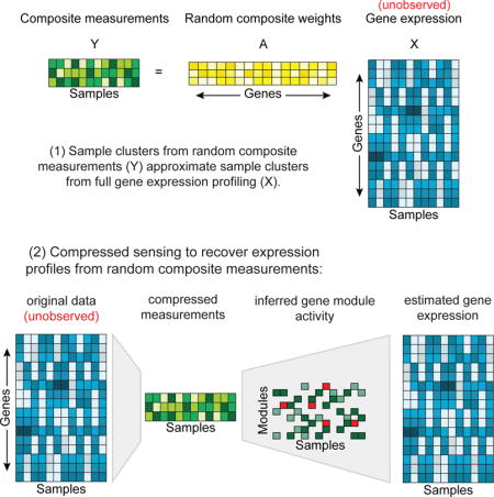
A composite measurement is a linear combination of gene abundances. Mathematically, it is the projection of a point in 20,000-dimensional expression space onto a single dimension, defined by a linear combination (weighted sum) of the 20,000 expression levels. In a simple case, this could be the sum of two gene abundances, but we will also consider measurements composed of up to thousands of genes (e.g. with nonzero weights for every gene). In a random composite measurement, the weights in the linear combination are chosen randomly. Making multiple composite measurements of a sample means taking multiple such linear combinations (Figure 1A, STAR-Methods). We formally represent the projection from high-dimensional expression levels to low-dimensional composite measurements as:

$$Y=AX$$

where the matrix X ∈ ℝ^{g × n} represents the original expression values of n samples in g=20,000-dimensional space; the matrix A ∈ ℝ^{m × g} is the weights of m random linear combinations (here, we use Gaussian i.i.d. entries); and the matrix Y (m × n) is the samples in low-dimensional space.

Figure 1. Composite measurements of sparse module activity.

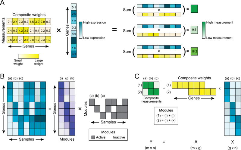
(A) Schematic example of three composite measurements (green, right) constructed from one vector of gene abundances (cyan). Each measurement is a linear combination of gene abundances, with varying weights (yellow) for each gene in each measurement. (B) Decomposition of gene abundance across samples by the activity of gene modules. The expression of genes (rows) across samples (columns) (left cyan matrix) can be decomposed into gene modules (purple matrix; rows: genes; columns: modules) by the modules’ activity (grey matrix, rows) across the samples (grey matrix; columns). If only one module is active in any sample (as in samples a, b, and c) then two composite measurements are sufficient to determine the gene expression levels (part C). (C) One such measurement (1) is composed from the sum of modules (i) and (j), and another (2) is composed from the sum of modules (j) and (k).

Mathematical results on low-dimensional projections (Dasgupta and Gupta, 2003; Johnson and Lindenstrauss, 1984) suggest that the pair-wise similarity of samples calculated in low-dimensional space Y can approximate their similarity in the original high-dimensional space, for example by a Euclidean distance. Under certain conditions, the distance between a pair of points in high-dimensional space can be well preserved with high probability when the data are projected onto a randomly defined m - dimensional subspace. Thus, according to theory, relatively small subspaces (e.g. m = 100) can be used to embed very high-dimensional data (e.g. g = 20,000; STAR Methods, Mathematical Details). Calculating distances in the low-dimensional space Y incurs a far lower computational cost.

This also suggests the possibility of an efficient way to collect expression data: rather than measuring the expression level of each of 20,000 genes individually, perhaps we could make m random composite measurements. If one composite measurement had the same cost as one individual gene measurement, there might be considerable cost savings in data collection, and we could use the low-dimensional data to learn about the correlations among the expression profiles of the samples. (Moreover, as discussed below, we can use low-dimensional data to recover information about the abundance of the 20,000 individual genes.) In the final Results section, we present pilot experiments addressing the technical feasibility of such a scheme.

Expression data to assess applicability

To empirically assess this and subsequent theoretical observations, in our analyses below, we used 41 previously-generated and publically available datasets containing a total of 73,608 unique expression profiles (table S1, STAR-Methods), from both bulk tissue samples and single cell RNA-Seq. These data were generated with diverse technologies, and we performed only minimal normalization to ensure robustness to the method of data collection (STAR-Methods).

Similarity of expression profiles: Application

To test the method, we applied it to each dataset, comparing the pairwise distances in the original high-dimensional space X (full original dataset), with those between samples as represented in the low-dimensional embedding, Y (compressed dataset). With only m=100 random composite measurements, the Pearson correlation coefficient (averaged across the datasets) between the distances in the low- and high-dimensional spaces was 94.4%. With m=400 random measurements, the average correlation was 98.5%.

Experimental measurements will inevitably include noise. We assume in all calculations below that the noise process for each gene in each sample is identically and independently distributed (i.i.d.) as a Gaussian, with an overall signal-to-noise ratio (SNR) of 2. (The results are robust to other choices of SNR, data not shown.) With m=100 noisy measurements, the average correlation between low and high dimensional distances was 84.5%; with 400 noisy measurements, the average correlation was 95.1% (Figure S1A,B; Pearson correlation, all p-values < 10⁻²⁰). The number of samples in a dataset had little impact on this behavior (Figure S1B), but the fraction of datasets with high average correlation (>90%) increased exponentially as the number of measurements was increased (Figure S1C).

We tested whether nonlinear structures can be preserved, by comparing non-linear embeddings generated by either of two methods of manifold learning (Multidimensional Scaling (MDS) (Borg and Groenen, 2005) and Isomap (Tenenbaum et al., 2000), STAR-Methods), computed from full profiles or from 100 composite measurements. The average correlation between these distances was 57% for MDS and 54% for Isomap, suggesting that some, but not all, of the nonlinear structure was preserved.

Sample clustering is also preserved with composite measurements. For example, tissue-specific clustering patterns across the GTEx dataset of 8,555 samples from 30 tissues (Figure 2A) are mirrored exceptionally well in clusters based on 100 composite measurements in each sample (Figure 2C). Most deviations (e.g. cluster 28) are also observed in clusters of high-dimensional data with the addition of noise (Figure 2B), indicating that these are not the result of information loss in low dimension. The overall similarity between the two clusterings as defined by their mutual information (STAR- Methods) was 87% for the GTEx data. The mutual information was lower in datasets where clusters were not as obvious – e.g., when the samples are all derived from the same tissue, as in each of the 33 individual TCGA tumor types (36%, on average). This reflects some loss of information about clustering in low dimension, but also the fact that the high dimensional clusters themselves are not inherently well-separated (and are indeed more impacted by the addition of noise; Figure S1D). Even so, the distances themselves are well preserved from high to low dimension in these cases (84% correlation; Figure S1A).

Figure 2. Clusters based on composite measurements match high-dimensional clusters.

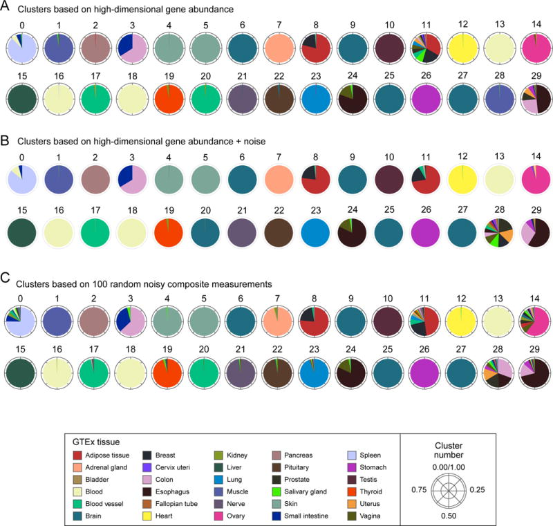
Shown are 30 clusters of GTEx samples (0–29; arbitrary order) based on (A) expression of 14,202 genes, (B) gene expression plus the addition of random noise (SNR=2), or (C) 100 random noisy composite measurements. Clusters in both (B) and (C) match the original clusters, with 91% and 87% mutual information, respectively (cluster numbers were manually reassigned to align with (A)). Each pie chart corresponds to one cluster and shows the composition of samples in the clusters by the individual tissues (colors, legend). Deviations from the original clusters which appear in both (B) and (C) (e.g. cluster 28) likely indicate the effects of noise, rather than loss of information in low dimension.

As a comparator of how far these random composite measurements are from being optimal, we compared them to the top 100 principal components (PCs; the optimal linear embedding). These PCs preserved nearly all of the high dimensional information, both distances and clusters (such that the average correlation between PC and composite measurement distances was 84%, versus 84.5% above).

Finding modular structure in order to recover gene abundances from low-dimensional data: Theory

Next, we wish to “decompress” the measurements, that is, recover the abundance of each of the individual 20,000 genes from random composite measurements. In compressed sensing, this is possible provided that the high dimensional data possess a sparse structure in some representation (Candes et al., 2005; Donoho, 2006). (STAR Methods, Mathematical Details and reviewed in (Eldar and Kutyniok, 2012)). Gene expression data is highly structured (Alter et al., 2000; Bergmann et al., 2003; Prat et al., 2011; Segal et al., 2003); if we can find this latent structure, we could leverage it to decompress the compressed measurements.

The challenge in recovering high-dimensional data from low-dimensional observations centers on the underdetermined system of equations:

$$Y=A\widehat{X}$$

where Y and A are known, and we wish to estimate $\widehat{X}$, the predicted expression levels in 20,000-dimensional space. If gene expression is arbitrarily complex (that is, if the abundance levels of each gene may vary across samples independently from all other genes), it will be impossible to infer the gene expression pattern from a small number of measurements. Conversely, if some genes are co-regulated and thus their abundances covary in sets (“modules”), then we can consider the alternative – and potentially easier – problem of using composite observations to determine the activity level of each module in each sample. The more that gene expression follows a ‘modular’ structure, the better the prospects of recovering the 20,000 abundances from far fewer measurements.

We formalize the notion of modular activity in the following way. Suppose there is a “dictionary” of d modules given by a matrix, U ∈ ℝ^{g × d}, with each column of the matrix describing one module. The activity level of each module in each sample, represented by a matrix W ∈ ℝ^{d × n}, approximates the observed expression profiles as X ≈ UW . Thus, the description of modular activity can be posed as a matrix factorization.

As a toy example, consider a fundamental dictionary of 500 gene modules, where each sample may activate at most 15 at a time. In the terminology of compressed sensing, we would say that samples used gene expression patterns that were “k-sparse”, with k = 15. (For practical purposes, it will be enough that samples’ gene expression patterns can be approximated by such a representation—that is, they are approximately k-sparse.) If expression were truly structured in this way, this could allow us to compress and decompress biological measurements. For instance, if the dictionary had only three fundamental modules, and each cell activated only one of these modules (Figure 1B), then with only two measurements we could infer which of the three modules is active (Figure 1C). Thus, because the dictionary is both small and sparsely used, we can recover gene expression from a number of measurements that is smaller than both the number of genes and the number of modules (that is, 2 vs. 20,000 and 3).

Modular activity in gene expression profiles: Results

We considered three algorithms for matrix factorization in the context of compressed sensing. Two algorithms, Singular Value Decomposition (SVD) (Alter et al., 2000) and sparse nonnegative matrix factorization (sNMF) (Mairal et al., 2010), are commonly used. We also developed a third algorithm, Sparse Module Activity Factorization (SMAF), which is particularly suited to our needs, because it identifies a non-negative, sparse module dictionary, and sparse module activity levels in each sample. Sparsity constraints in the dictionary and the activity levels are designed to facilitate both compressed sensing and biological interpretation. Dictionary sparsity reduces redundancy between modules, making interpretation easier, and also increases dictionary incoherence (a statistical property that captures the suitability for compressed sensing). Further details for each algorithm are in the STAR Methods, Mathematical Details.

We assessed the performance of SVD, sNMF, and SMAF, using each to calculate module dictionaries and module activity levels for each dataset. For each method, we quantified the ability of the model to fit the data, the effective number of genes per module, the number of active modules per sample, as well as the “biological distinction” of the modules (i.e. the degree to which the dictionary modules are enriched in different functional gene sets curated in external databases (Liberzon et al., 2011); STAR- Methods).

While SVD, which is unconstrained, provided the best fit of the data (Table S2), its representations were not sparse (Figure 3A and S2A). Conversely, the sparsityenforcing methods sNMF and SMAF provided good fits as well (Figure 3C and Table S2), while generating sparse solutions (Figure 3A and S2A), which should enhance their performance for compressed sensing. Most importantly, SMAF generated dictionaries that were compact (Table S2), sparsely active (Figure 3A and S2A) and biologically distinctive (Figure 3B), whereas the enriched gene sets for each module in the SVD and sNMF dictionaries were largely redundant (Figure 3B). Finally, because they have reduced redundancy, SMAF dictionaries are more incoherent than those of sNMF (Figure S2C), suggesting that they should generally perform better in compressed sensing.

Figure 3. Sparse Modular Activity Factorization (SMAF) for gene expression.

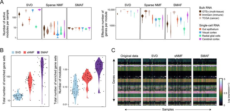
(A, B) Performance of different matrix decomposition algorithms. (A) Violin plots of the distribution of the number of active modules per sample (y-axis, left), and the effective number of genes per module (y-axis, right) for each of three methods, across different datasets (x axis, legend). (B) Violin plots of the total number of enriched gene sets across all modules within a dataset (left), and total number of enriched gene sets divided by the number of modules (right), for each of the three different algorithms. Each dot represents one dataset. (C) Original data, and reconstructed high-dimensional gene expression levels for each algorithm. Heat maps show, for the GTEx dataset the original gene expression profiles (left; 8,555 samples, 14,202 genes) and the profiles reconstructed from SVD, sNMF, and SMAF.

Using sparse modularity to recover gene expression profiles with compressed sensing: Theory

Next, we use the algorithms in a framework that would allow us to recover expression profiles from low-dimensional data generated by random, noisy composite measurements. Suppose that (1) we already know a high-dimensional dictionary U (learning it from initial training data using one of the algorithms), and (2) we have a set of composite measurements, Y = A(X + noise) produced with a known random matrix A. We ask whether it is possible to learn the weighted activity levels W for the modules corresponding to the high-dimensional data—and thereby recover the high-dimensional expression data X ≈ UW (Figure 4A). (We address later the harder problem blind compressed sensing: recovering X without information about U).

Figure 4. Compressed sensing of gene module activity levels.

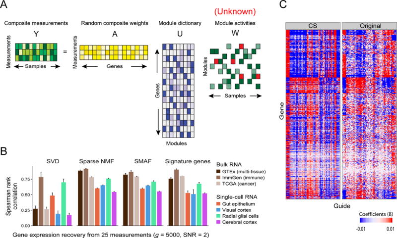
(A) Schematic of the core problem: composite measurements (Y, green) are used with composite weights (A, yellow) and a module dictionary (U, purple) to infer sparse module activities (W, green and red). (B) Performance of compressed sensing in recovery of expression levels. Shown are the Spearman rank correlation (y-axis, mean with error bars indicating standard deviation across 50 random trials) between the original data and 5,000 gene abundance levels recovered from either 25 measurements using module dictionaries found by different algorithms (SVD, sNMF, and SMAF) or by predictions from signature gene measurements based on models built in training data. (C) Performance in gene network inference. Gene networks were inferred from high-dimensional Perturb-Seq data (right) or from data recovered by compressed sensing (left; 50 composite measurements). Heatmap depicts the network coefficients (color bar) of 67 guides (columns) targeting 24 TFs and their 1,000 target genes (rows). The coefficients in both versions (CS and Original) are significantly correlated (50%; p-value < 10⁻²⁰).

To show this, we partition each high-dimensional data set X into a set of training samples, X_training, and a test set, X_testing (STAR-Methods). We apply each of the three algorithms to the training set to calculate a module dictionary via matrix factorization:

$$X_{\mathit{\text{training}}}\approx UW$$

We then simulate random composite measurements on the test samples:

$$Y=A\left(X_{\mathit{\text{testing}}}+\mathit{\text{noise}}\right),$$

where the matrix A defines the random composition of g genes in each of m measurements (as before, with m ≪ g). Next, for a given module dictionary (U_SVD, U_NMF, ^or U_SMAF), we find the module activities, $\widehat{W}$, that best fit our composite observations (Figure 4A), such that:

$$Y\approx AU\widehat{W}$$

This optimization is performed while enforcing k-sparsity in $\widehat{W}$, so that there are no more than k active modules per sample. Finally, we use the module activity coefficients in each test sample to compute predicted gene expression values, $\widehat{X}=U\widehat{W}$, and compare these predicted values with the actual values. The results are three sets of predictions, ${\widehat{X}}_{\mathit{SVD}}$, ${\widehat{X}}_{\mathit{NMF}}$, and ${\widehat{X}}_{\mathit{SMAF}}$.

Compressed sensing: Results

We applied this approach to each dataset, using 5% of the samples in each for training, and 95% for testing. We assessed how well we recover full profiles from composite measurements, and found that sparse dictionaries from sNMF and SMAF performed well, whereas the non-sparse ones from SVD did not (Figure 4B, Figure S3A). For example, in the GTEx data set with 25 random, noisy composite measurements of 5,000 genes, the predicted profiles showed an average Spearman rank correlation with the original values (calculated across all genes and testing samples) of 88% for sNMF and 82% for SMAF, but only 26% for SVD (averaged over 50 trials with different random training samples, testing samples, composite weights, and genes; Figure 4B). With only 10 composite measurements we obtained surprisingly good accuracies of 83% for sNMF and 79% for SMAF (Figure S4A). Thus, consistent with theory, successful recovery of gene expression from compressed measurements rests on samples having a sparse representation in the given dictionary—that is, on there being not too many active modules in each sample. Notably, SMAF – which represents each sample with 15 active modules chosen from a dictionary U of several hundred – also has substantially better performance than k-SVD – which represents all samples with different activity levels of the same 15 modules (corresponding to the top k eigenvectors, k = 15) (Figure S4).

Some features of gene expression variation were not captured as well as others. On average, the approach more accurately estimated the relative abundance of genes within an individual sample than the relative abundance of an individual gene across many samples (Figure S4B). The performance was also generally worse for expression datasets from single-cells than from bulk tissue (average Spearman correlation of 62% vs. 87%, for 25 composite measurements). This can be partially explained by the effect of the skewed distributions in single cell expression profiles (Kharchenko et al., 2014; Shalek et al., 2014): the observed abundances are generated by a zero-inflated Poisson process, whereas our optimization methods model the data as normally distributed. Indeed, the difference between Spearman and Pearson correlation is most drastic in single cell datasets (Figure S4C). Two additional sources of noise could affect performance: intrinsic noise (e.g., transcriptional bursting (Deng et al., 2014)), which is not shared across genes in a module; and technical variability, if not shared across cells.

One potential limitation is the degree to which a dictionary learned on one dataset can be successfully applied to new datasets that are biologically distinct. To test this, we partitioned each of the 33 individual tumor types in the TCGA catalog to a 5% training and 95% testing set, learned a dictionary from each of the 33 training sets, simulated composite measurements in each of the testing sets (m=25, g=5,000, SNR=2), and used each of the 33 dictionaries to decompress measurements from each of the 33 test sets (same tumor type and the other 32 types). In general, using a dictionary derived from a different tumor type resulted in reduced performance (from 87% to 68% on average with SMAF; Figure S3B,C). Using a SMAF dictionary from a related tumor type often resulted in better performance (Figure S3B). SMAF performed considerably better than SVD and sNMF in this analysis (Figure S3C).

Decompressed profiles perform well in downstream network inference

We also tested the utility of data recovered by compressed sensing in downstream analysis, focusing on gene network inference from genetic perturbations. We used a published Perturb-Seq screen (Dixit et al., 2016) in LPS-stimulated dendritic cells, where 24 TFs were perturbed in a pool by 67 sgRNAs followed by single-cell RNA-Seq, profiling 11,738 genes in 49,234 cells. We randomly selected 5% of the data for training, used these to learn a module dictionary with SMAF, simulated 117 composite measurements on the testing data (100-fold under-sampled; SNR=10, with lower added noise because the data are inherently very noisy), recovered the module activities, and predicted gene expression profiles. The recovered expression profiles had a 46% Spearman correlation (92% Pearson) with the original data. For comparable undersampling, this was the worst performance among the tested datasets, reflecting both technical variation in single cell RNA-Seq, and the fact that the samples were all the same cell type with subtle differences between them.

Nonetheless, using the decompressed data $\left(\widehat{X}\right)$ for network inference (as in (Dixit et al., 2016)) showed good agreement with a network model learned on the original (full) dataset (X) (Figure 4C). The inference algorithm uses the TFs targeted for perturbation in each cell (encoded in sgRNAs barcodes) to learn a matrix, β, of coefficients describing positive and negative association between each of 24 perturbed TFs and the 11,738 target genes. (In our simulations, sgRNA barcodes were not part of the composite measurements.) The correlation between the two sets of coefficients (β and $\widehat{\beta }$) was 35% (p-value < 10⁻²⁰), averaged across simulation trials. When we restrict the network inference problem to a subset of ~1,000 variable genes (e.g. those that are significantly up- or down-regulated after stimulus; m=50 measurements), performance was further improved. The recovered variable gene levels were 72% Spearman correlated (93% Pearson) with the original levels, and the inferred networks (using only variable genes as targets) were 49% correlated (Figure 4C). Finally, we used unperturbed data to calculate variable genes and a module dictionary (training set), and performed compressed sensing and network inference on perturbed data (testing set), again obtaining networks that were significantly correlated with those obtained from the original data (39%).

Recovering gene modules and activity levels from random compositional measurements without knowledge of expression patterns: Theory

Suppose we have neither a high-dimensional dictionary nor training data; can we still learn a dictionary U from only the low-dimensional composite measurements? In other words, in the equation:

$$Y\approx A\widehat{X}\approx A\widehat{U}\widehat{W}$$

can we learn the module dictionary $\widehat{U}$ based only on knowledge of the low-dimensional data Y and projection matrix A ? Once we have the dictionary $\widehat{U}$, we can apply the methods of compressed sensing described above to recover the module activity levels, $\widehat{W}$, and the original gene abundances, $\widehat{X}$. In the compressed sensing field, this problem is called “blind compressed sensing” (BCS).

Remarkably, the blind compressed sensing problem can be solved under certain conditions (Aghagolzadeh and Radha, 2015; Gleichman and Eldar, 2011; Pourkamali-anaraki et al., 2015). Early work (Gleichman and Eldar, 2011) showed that if the dictionary is one of a known, finite set, or if it obeys certain structural constraints, it can be recovered solely from compressed observations, but these constraints are not relevant for gene expression. Subsequent empirical (Pourkamali-anaraki et al., 2015) and theoretical (Aghagolzadeh and Radha, 2015) studies have shown that using variable measurements (e.g. a different random Gaussian matrix A_i for each sample) allows one to recover the dictionary without restrictive constraints (but still assuming dictionary incoherence and sparse module activity; STAR Methods, Mathematical Details). Unfortunately, the practical value of existing algorithms such as CK-SVD (Pourkamali-anaraki et al., 2015), is limited for the gene expression domain, since they practically require large number of samples (e.g. 50,000) with very low noise (e.g., SNR of 25) to learn small dictionaries (e.g. 15 modules).

We thus developed BCS-SMAF (Figure 5A), a new algorithm for blind compressed sensing in the context of gene expression. BCS-SMAF uses fixed and variable measurements, while also leveraging dictionary constraints (as in SMAF) that are appropriate for analyzing gene expression, especially the observation that similar samples activate similar dictionary modules (Figure S2D). In a nutshell (for details and theoretical underpinnings see STAR Methods, Mathematical Details), BCS-SMAF first clusters samples based on the subset of composite observations; within each cluster, it searches for a relatively small dictionary (e.g. with 15 modules) to explain the samples in that cluster; it then concatenates the small dictionaries into a large dictionary. This provides initial values for U and W, upon which it iterates, using for each step of the update all available measurements for each sample, until termination.

Figure 5. Blind compressed sensing (BCS) of gene modules.

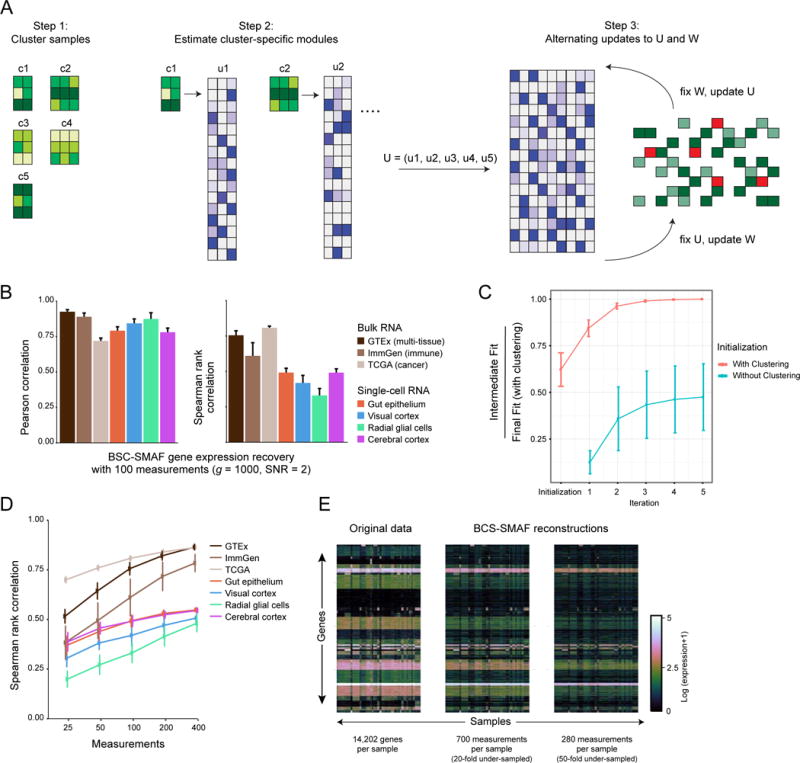
(A) BCS-SMAF steps. (1) Samples are clustered based on composite observations; (2) Small module dictionaries are estimated separately for each cluster, and concatenated into a large dictionary; (3) Procedure alternates over updates to the module dictionary and activity levels. (B–E) Performance of BCS-SMAF. (B) Bar plots of the Pearson (left) and Spearman (right) correlation coefficients (Y axis) between predicted and actual gene abundances. (C) Convergence of BCS-SMAF. The intermediate fit at each iteration as a fraction of the final fit (with clustering initialization) (Y axis), averaged across all datasets and random trials, when the algorithm can be initialized via clustering (red line), or randomly (teal line). (D) Spearman correlation coefficients (Y axis), as in (B), for varying numbers of composite measurements (X axis). Error bars in (B–D) represent one standard deviation across 50 random trials. (E) Original (left) expression levels for all 14,202 genes in GTEx and their corresponding predictions by applying BCS-SMAF to 700 (middle) and 280 (right) composite measurements.

Blind Compressed Sensing for recovering gene expression profiles: Results

We first applied BCS-SMAF to simulated data in random trials (STAR- Methods). We found that (1) the algorithm converged quickly (in ~5–10 iterations) (Figure S4D); (2) blind recovery was more difficult when samples had a denser representation (i.e. for larger k) (Figure S4E); and, (3) it is more difficult to reconstruct modules that are activated by fewer samples (Figure S4F). BCS-SMAF did not always converge to the same dictionary given different starting samples, suggesting an area for future improvements.

We next tested BCS-SMAF on our expression datasets. We simulated noisy composite measurements, y_i = A_i(x_i + noise), across a randomly selected subset of genes (g = 1000, signal-to-noise ratio: 2), and varied the number m of composite measurements (from 2.5- to 40-fold fewer than the number of genes). We compared the expression levels recovered from BCS-SMAF with the original values. (Because BCS-SMAF takes longer to run, we decreased the number of genes to efficiently run many random simulations.)

Although performance was expectedly worse than results with a known dictionary, the recovered abundance levels were substantially correlated with the original values (Figure 5B). For the GTEx data with g = 1000 genes and m = 100 composite measurements (10-fold under-sampling), the expression profiles recovered by BCS-SMAF had on average a Pearson correlation of 92% and Spearman correlation of 76% with the true values (compared with 93% and 88% for compressed sensing with a known dictionary). Performance dramatically improved as the number of composite measurements increased; for instance, increasing from 25 to 400 measurements, Spearman correlations increased from 52% to 86% for GTEx (Figure 5D). BCS-SMAF converged quickly (~5 iterations), and initialization by clustering yielded considerably better results (Figure 5C).

Tested on all 14,202 genes in the GTEx dataset (SNR 2) with 20-fold (m = 700) to 50-fold (m = 280) fewer composite measurements than genes, BCS-SMAF produced effective results based on overall correlation, sample clustering and even biological distinctiveness. We obtained acceptable Spearman correlations of 71% and 56% with the original values, respectively (93% and 88% Pearson) (Figure 5E). Sample clusters generated from the BCS-SMAF reconstructed data agreed well with the original clusters (Figure S1E, 81% and 75% mutual information, respectively). Even when reconstructed clusters deviate from the originals, they were still often useful in the sense that they correctly grouped samples by tissue (e.g. clusters 0, 17, 18, and 26; Figure S1E). BCS-SMAF also produced dictionaries with less redundancy and greater biological distinctiveness of modules than those found by applying SVD or sNMF to the original data (0.29 unique gene sets enriched per module with BCS-SMAF versus 0.15 and 0.06 with SVD and sNMF). Finally, BCS-SMAF modules and their activities can produce meaningful biological insight. For instance, all ten samples with highest activity in BCS-SMAF (20-fold under-sampled) module 169 are derived from skeletal muscle and the module is enriched in genes involved in respiration, generation of metabolites, muscle contraction and housekeeping genes.

Differences between composite measurements and signature gene analysis

A simple alternative to performing random composite measurements is using the training phase to select a set of individual “signature genes” for measurements (Biswas et al., 2016; Donner et al., 2012; Peck et al., 2006; Subramanian et al., 2017), along with learning a model to predict the remaining genes from this measured set.

The two strategies have distinct advantages and drawbacks. Signature gene measurements are straightforward to understand and to implement in practice, but the measurement design may change as the biological context shifts. In contrast, random composite measurements—because they are random—are broadly suitable for different contexts. Thus, while signature gene methods require some similarity of the measured samples to those used to train the model, composite measurements can be used to recover expression levels blindly in new samples with BCS-SMAF. Although signature gene measurements can be used without imputation for pairwise comparison (and clustering) of samples (e.g., (Duan et al., 2014)), our empirical results show that 100 signature genes do not preserve sample-to-sample distances as well as 100 composite measurements (59% vs. 81% Pearson correlation over all pairwise distances, averaged across all datasets, Figure S5A). For recovery of unobserved expression levels in testing data after model building in training data, at moderate levels of noise, the two methods have similar performance, but the performance of signature genes deteriorated more quickly as noise increased (Figure S5B). This reflects the fact that composite measurements tend to cancel out the (uncorrelated) noise in each gene, while signature measurements are highly sensitive to noise in individual genes. This feature could be particularly relevant in noisy single-cell RNA-Seq data (Wagner et al., 2016).

Making composite measurements in the laboratory: Theory

We next consider the challenge of implementing compressed sensing with a lab protocol that measures a linear combination of the expression levels of a set of genes, S, without having to determine the levels of the individual genes,

$$y={\displaystyle \sum a_i{x}_i;\mathit{where}i\in }S$$

If all weights are equal, probes for the genes could be combined in equal proportions on the same “channel”.

For RNA abundance (Figure S5C), probes might consist of oligonucleotides targeting each gene in the set, a measurement channel could be encoded in a sequence barcode attached to the oligonucleotides, and a measurement would consist of the net abundance of the (hybridized) barcode of the channel. To extend to unequal weights, the relative abundance of probes targeting each gene in a set is adjusted proportionally, if the weights a_i are all positive (we extend below for negative weights). One implementation would create a pair of a single-stranded DNA probes, L_i and R_i, that hybridize to adjacent locations on the mRNA of gene i, so that they may be ligated with an enzyme that selects for RNA-DNA hybrids (such as in (Lohman et al., 2014)). The left and right probes L_i and R_i contain a left and right barcode sequence, respectively, which are each the same for all the genes measured. To perform a composite measurement, we: (1) create a weighted pool consisting of all of the probe pairs; (2) hybridize the mixture to mRNA in a fixed sample; (3) perform ligation; (4) wash away the un-hybridized and un-ligated products; and (5) measure the total amount of the barcode (Figure S5C). To extend to negative weights, we can make two separate composite measurements, y₊ and y₋, corresponding to the positive and negative coefficients, and subtract the second from the first. We can also perform m composite measures simultaneously by hybridizing 2m pools corresponding to the positive and negative coefficients of each linear combination and measuring barcode abundance. Notably, probe hybridization needs to be linear in the amount of mRNA, and in the concentration of probes. Furthermore, because hybridization efficiency will not be identical across probes, we should learn it by performing the procedure on diverse mRNA samples for which the ground truth is known from a hybridization-independent assay, such as RNA-Seq. We can also use multiple probe pairs per gene. While it is natural to perform the final readout by qPCR, barcode sequencing is also a possibility. The library of sequenced molecules is very complex, but it should be possible to estimate the relative abundances of the barcodes with shallow sequencing.

Composite measurements could also be performed with proteins. One approach could leverage methods in mass cytometry in single cells (CyTOF) (Bendall et al., 2011) or in situ (MIBI (Angelo et al., 2014) and IMC (Giesen et al., 2014)), where multiple antibodies, barcoded with heavy metals, are bound in multiplex. Readout currently has a fixed number of channels corresponding to ~100 heavy metal ions. Applying compressed sensing – by generating weighted antibody pools with the same barcode – could expand the panel of targets by an order of magnitude or more.

To scale these methods to thousands or tens of thousands of genes, we will need to address practical concerns of building large composite libraries. More practical compositions with random subsets of genes and equal (i.e. binary) weights are also suitable for compressed sensing. For example, using random subsets of 100 equally-weighted genes in GTEx gives nearly the same correlation as random Gaussian measurements (82% vs. 81%; g=5000, m=25). Our methods are robust to noise in the compositional weights, which might be introduced during probe library preparation (82% vs. 80% correlation with an SNR of 2 in the composite weights; GTEx, g=5000, m=25). Finally, it may be advantageous to bias the weights towards a set of “key” genes, such as transcription factors, which tend to be lowly expressed. We can increase sensitivity to these genes by their giving them stronger weights or by biasing the inference task towards minimizing the error on these genes.

Making composite measurements in the laboratory: Results

We tested our strategy by performing a modest proof-of-concept experiment. We measured by a composite approach the levels of 23 transcripts in K562 cells (selected to capture a range from highly abundant housekeeping genes to very lowly expressed ones). First, we established our procedures by measuring individual genes by our assay (comparing our protocol to standard qPCR), and showed that correlations improved when we used four pairs of probes targeting different positions within each gene, all using the same barcode (ranging from 39% to 88%; Table S3). Next, we compared the single gene results to using composite measurements. We designed 20 arbitrary sets of composite measurements by taking random linear combinations of the 23 genes (with weights randomly selected from four concentrations spanning four orders of magnitude; Table S4) and created the corresponding probe libraries. With two replicates using different measurement barcodes, we observed 85% and 90% correlation between the observed results and the expected values calculated directly from the linear combinations of individual gene abundances (Figure S5D).

Discussion

Building on established mathematical frameworks, we have demonstrated several results that may be initially unintuitive in biology. Below, we provide guidance for applying these ideas in the development of future experiments.

Several important limitations arise from information loss during compression and decompression. Information loss during compression can lead to a distortion of sample similarity, making it difficult to distinguish similar samples. We observed this in the analysis of datasets consisting of very similar samples (e.g., individual TCGA tumor types, single-cell RNA-Seq of cells stimulated with LPS). Further information loss during decompression can lead to errors in the estimation of high-dimensional gene expression. This can occur if expression levels cannot be accounted for by modular activity (e.g. single-cell “bursting”), or if the dictionary modules are biased or inaccurate. In the setting with training data, a biased dictionary could arise if the training data are not representative of testing data. In the blind setting, if very few samples share a module, then it will be difficult to infer. Even if the modules are correctly specified, the core premise of compressed sensing (using composite measurements to infer module activity) may not be appropriate for some applications. For instance, cis-eQTLs typically affect the expression of one gene, not an entire module.

With these limitations in mind, we can envision various applications of composite measurements. For instance, in methods like Perturb-Seq (Adamson et al., 2016; Dixit et al., 2016) pooled CRISPR screens are combined with single cell RNA-Seq. However, these methods do not allow for the a priori selection of cells with specific expression patterns; the number of perturbations that can be studied is thus limited by costs. Even though such data can only be partially recovered by compressed sensing, it suffices to infer gene network models. Compressed sensing could also allow selection based on expression patterns. For example, one might (i) learn to recognize a complex expression pattern based on a handful of composite measurements; (ii) create probe sets for each composite measurement carrying a different fluorescent label; (iii) perform composite measurements on fixed, permeabilized cells; (iv) select cells carrying the signature by multi-dimensional FACS sorting; and (v) examine the proportion of barcodes in selected and unselected cells.

Molecular compressed sensing can also be applied to the measurement of proteins. Compressive proteomics could be possible with mass cytometry, especially imaging mass cytometry (Giesen et al., 2014), where protein abundance information is spatially resolved to produce an “image” of a fixed sample. With composite measurements, these images could potentially be expanded to include information on thousands of proteins (for reference, above we demonstrate 85% Spearman correlation, average across datasets, in recovering 5,000 mRNA abundance levels from 50 composite measurements).

Compressive measurement may be useful for other biological systems that may possess a sparse modular structure. Chromatin landscapes, for example, are also patterned into subsets of the genome that co-vary in chromatin state across subsets of conditions (Consortium et al., 2015). Other high-dimensional signals such as the spliceosome or metabolome might be similarly structured.

With any of these applications, we wish to make efficient measurements of a high-dimensional signal. Given that co-regulation (and thus, modularity) of high-dimensional variables is a relatively ubiquitous phenomenon across biological systems, we anticipate that the ideas presented here will have broad applicability.

STAR Methods

Contact for Reagent and Resource Sharing

Further information and requests for resources and reagents should be directed to the Lead Contact Aviv Regev at aregev@broadinstitute.org.

Experimental Model and Subject Details

K562 cell cultures

Human chronic myelogenous leukemia (CML) K562 cells were cultured as recommended by ATCC. Briefly, cells were maintained in Iscove’s Modified Dulbecco’s Medium (IMEM) supplemented with 10% FBS (HyClone), 2 mM GlutaMAX (Life Technologies), 100 U/ml penicillin, and 100 μg/ml streptomycin at 37°C with 5% CO₂ incubation. Cells were seeded at a density of 1 million cells per mL for each subculture and a minimum of 2 million cells were used for each RNA extraction.

Method Details

Mathematical Details

Compressed sensing (CS) encompasses algorithms and a formalism for analyzing the necessary and sufficient conditions for high-dimensional signal recovery from noisy, incomplete measurements. For a thorough mathematical review of the theory and applications of compressed sensing we point the reader to (Eldar and Kutyniok, 2012). Here, we briefly review the critical aspects of CS, note their particular applicability to gene expression profiling, and provide a more detailed account of our BCS-SMAF algorithm.

Random projection into low-dimensional space and the Johnson-Lindenstrauss lemma

Though not directly invoked in CS, the Johnson-Lindenstrauss lemma (Johnson and Lindenstrauss, 1984) provides a good foothold for understanding bounds on distortion in low dimension. We will be concerned with distortion of distances between (1) pairs of gene expression profiles (for the purpose of calculating sample similarity), and (2) pairs of gene modules (for compressed sensing). We will begin by stating the lemma and showing how an intermediate step in a proof of the lemma allows us to understand sample similarity, before moving to compressed sensing in the next section.

Lemma (Johnson-Lindenstrauss): There exists a Lipschitz mapping from high to low dimension, f : ℝ^g → ℝ^m, for any set of n points, such that for any two points, u, v, if $m\ge 0\left(\frac{\log n}{{\epsilon }^2}\right)$, then

$$\left(1-\epsilon \right){\Vert u-v\Vert }^2\le {\Vert f(u)-f(v)\Vert }^2\le {\Vert u-v\Vert }^2(1+\epsilon ).$$

For our purposes, the function f will correspond to a measurement matrix A so that $f(x)=\frac{1}{\sqrt{g}}Ax$ for a vector x with g entries, with A consisting of Gaussian i.i.d. entries with mean 0 and standard deviation 1. We will refer to A as a composite measurement matrix, with m measurements composed of g genes.

Our analytical understanding of the preservation of distances with composite measurements comes from a proof of the JL-lemma (Dasgupta and Gupta, 2003). This proof begins by demonstrating (via lemma 2.2) that the probability of distance preservation within 1 ± ε is

$$\mathrm{Pr}\left((1-\epsilon ){\Vert u-v\Vert }^2\le {\Vert \frac{1}{\sqrt{g}}A(u-v)\Vert }^2\le {\Vert u-v\Vert }^2(1-\epsilon )\right)\ge 1-2e^{-\frac{\left(\frac{{\epsilon }^2}{2}-\frac{{\epsilon }^3}{3}\right)m}{4}}.$$

Thus, the probability that the distance between a pair of gene expression profiles is distorted beyond 1 ± ε decreases exponentially as the number of composite measurements grows. This is reflected empirically with noisy composite measurements of gene expression in Figure S1A–B, in which the correlations between high- and low-dimensional distances in each data set are shown for different values of m, and in Figure S1C, in which the frequency of distortion (below a correlation of 90%) is shown to decrease exponentially with increasing m.

While the correlation between high- and low-dimensional distances does not depend on the number of samples (n), in order to guarantee that all pairwise distances among the n points are preserved with high probability, the number of measurements must increase as the number of samples increases. The remainder of the proof of the JL-lemma demonstrates the surprising result that m only needs to grow as $O\left(\frac{\log n}{{\epsilon }^2}\right)$. To see how this relates to the recovery of gene expression profiles from composite measurements, we next introduce some basics of compressed sensing.

Compressed sensing and null space conditions for sparse signals

Suppose that a gene expression matrix, X ∈ ℝ^gxn, can be factorized into a module dictionary and module activity levels, X = UW, such that, for each column of W ∈ ℝ^dxn there are exactly k nonzero values (we say that W is column-wise k-sparse). Each column of U ∈ ℝ^gxd is a description of a module. Given composite measurements, y, of a sample, x, we wish to recover the module activity levels so that

$$y=Ax=\mathit{AUw}.$$

This is the core problem of compressed sensing.

Suppose that we have the true sparse activity levels, w, and a distinct k-sparse vector w′, such that x = Uw ≠ Uw′. If AUw = AUw′ then we will not be able to distinguish w from w′ based solely on y. The vector (w − w′) is in the null space of the matrix AU.

What conditions can we place on AU (and its null space) such that all such vectors w and w′ can be distinguished? Suppose that w and w′ are supported on disjoint modules, so that (w – w′) is 2k-sparse. If there are no 2k-sparse vectors in the null space of AU, then we are guaranteed to be able to distinguish the vectors based on y. This can be equivalently characterized by the spark of AU: The spark of a matrix is the smallest number of columns of the matrix that are linearly dependent. Then we have that for any set of composite observations y, there exists at most one k-sparse signal w such that y = AUw if and only if spark (AU) > 2k.

These null space conditions are useful for developing intuition about the separability of sparse solutions. Next, we review the core property of CS that tells us how many measurements we need for robust recovery.

The Restricted Isometry Property (RIP)

The matrix AU satisfies the RIP (Candes and Tao, 2004) of order 2k if there exists a δ such that, for all 2k-sparse vectors z

$$\left(1-\delta \right){\Vert z\Vert }^2\le {\Vert \mathit{AUz}\Vert }^2\le {\Vert z\Vert }^2\left(1+\delta \right).$$

We can interpret this as saying that AU approximately preserves the distance between any pair of k-sparse vectors. This is relevant for distinguishing solutions based on composite observations (suppose z = (w − w′); if ||z||² > 0 then we also want ||AUz||² bounded away from zero). The total possible number of k-sparse vectors that we want to be able to distinguish with composite measurements is 0(d^k). If the matrix AU is a random Gaussian matrix, then we can combine this result with the JL-lemma to say that the number of composite measurements should be at least

$$m\ge 0\left(\frac{k\log \left(d\right)}{{\delta }^2}\right)$$

for robust signal recovery with d modules in the dictionary U.

Another property, coherence, is commonly used to analyze the suitability of an arbitrary (i.e. not necessarily Gaussian) matrix AU. The coherence, μ(AU), is the largest absolute inner product between any pair of columns with unit norm. This is inversely related to the spark:

$$\mathit{spark}\left(AU\right)\ge 1+\frac{1}{\mu \left(AU\right)}.$$

If a matrix AU has unit-norm columns and coherence μ, then it satisfies the RIP of order k with δ = (k − 1) μ for all sparsity levels $k<\frac{1}{\mu }$.

To summarize: (1) as discussed in the main text and seen through the discussion above, sparsity is a key requirement for compressed signal recovery; (2) we can use the RIP to establish a lower bound on the number of measurements needed for robust recovery; and (3) incoherent matrices (AU) perform better. Thus, in order to recover gene expression profiles from a small number of random Gaussian measurements, we should seek to learn a dictionary that is sparsely activated and has distinguishable (non-redundant) modules.

Algorithms for learning a dictionary: SVD, sNMF, and SMAF

Several methods of matrix factorization are already commonly used for gene expression analysis. Two of the best-known algorithms are Singular Value Decomposition (SVD) (Alter et al., 2000) and nonnegative matrix factorization (NMF) (Mairal et al., 2010). For the purpose of compression, we desire an algorithm that can accurately represent gene expression with a small number of active modules (i.e. very few nonzero w_i,l coefficients). The general versions of SVD and NMF are not guaranteed to accomplish this, but modified versions, such as sparse NMF (sNMF, (Mairal et al., 2010)), incorporate sparsity constraints to enforce such behavior. However, methods like sNMF enforce sparsity in general in W but not specifically per sample. As a result, while the overall matrix may be sparse, some samples may activate very few modules and others very many modules, such that the model is less suited to the needs of compressed sensing and less compatible with our current understanding of gene expression. Moreover, the dictionaries found by sNMF can be dense with coefficients, which results in partially correlated, redundant modules (since every pair of modules will have some overlap in coefficients). Module redundancy can compromise compressed sensing by increasing the coherence of the dictionary.

We thus developed a third algorithm that is particularly suited to our needs. Our method, Sparse Modular Activity Factorization (SMAF), identifies a non-negative, sparse module dictionary, and sparse module activity levels per sample. SMAF introduces two changes compared to sNMF and similar methods. First, for the activity levels, it enforces k-sparsity; that is, each sample may activate no more than k modules (with k = 10 unless otherwise specified). Enforcing k-sparsity per sample, rather than only sparsity in general in W (as in sNMF), is appropriate for compressed sensing. Second, SMAF also enforces sparsity (via an l₁-relaxation) in the module dictionary, in order to reduce redundancy between the modules. With a fixed number of nonnegative modules, if each is sparse, then they are likely to have less overlap.

Formally, the optimization problem for SMAF is as follows: Given a gene expression matrix X ∈ ℝ^gxn find a module dictionary U ∈ ℝ^gxd and a module activity matrix W ∈ ℝ^dxn that minimizes:

$$\underset{U,W}{min}{\Vert X-UW\Vert }^2+\lambda {\Vert U\Vert }_1;$$

$$\text{such that }{u}_{i,j}\ge 0,\Vert u_{;,l}\Vert =1,\text{and}{\Vert w_i\Vert }_0\le k\forall i\in \{1,\dots ,n\}.$$

Our algorithm to solve this optimization problem proceeds with alternating updates to U and W.

Algorithm.

Sparse Module Activity Factorization.

1. SMAF(X, d, λ, k)

2. Initialize U ∈ ℝg × d and W ∈ ℝd × n randomly.

3. For 10 iterations:

a. Update the module dictionary as U = Lasso Nonnegative (X, W,λ).

b. Normalize each module so that ||ui||2=1.

c. Update the activity levels as W = OMP (X, U, k).

4. Return U, W.

In practice, we find the algorithm converges quickly, and, hence, 10 iterations in step 3 are sufficient. The subroutine OMP() corresponds to Orthogonal Matching Pursuit. It finds a solution to x_i = Uw_i, such that ||w_i||₀ ≤ k.

Blind Compressed Sensing with SMAF (BCS-SMAF)

The problem of blind compressed sensing is to recover a module dictionary and module activity levels given only composite observations. Formally, given:

$$Y=\mathit{AUW}$$

we use observations Y and composite weights A to recover both U and W. BCS is reducible to the problem of learning a good dictionary; once U is fixed, the methods of CS can be applied to learn the module activities. In the work that originally described the problem of BCS (Gleichman and Eldar, 2011), it was shown that, in addition to sparsity and coherence assumptions, structural constraints on U (e.g. the assumption that U consists of orthogonal block diagonal bases, or is chosen from a finite set of known bases) are needed to make the problem tractable. Constraining U according to structural assumptions on gene modules is intuitively appropriate, but the original constraints and accompanying algorithms are not relevant for our problem.

Subsequent empirical (Pourkamali-anaraki et al., 2015) and theoretical (Aghagolzadeh and Radha, 2015) work has shown that using variable measurements (e.g. a different random Gaussian matrix A_i for each sample) allows one to recover the dictionary without restrictive constraints. Below, we will briefly review these results, and then state the optimization problem for blind compressed sensing of gene expression and our algorithm to solve it.

Fixed vs. variable measurements

Recent work has shown that the use of variable measurements makes it possible to estimate modules from compressed observations (Aghagolzadeh and Radha, 2015; Pourkamali-anaraki et al., 2015). To see how, first suppose for simplicity that there is only one module in the dictionary (i.e. U ∈ ℝ^gx1 and W ∈ ℝ^1xn; this assumption is not required, but is used to illustrate the role of variable measurements). We wish to estimate U and W given our observations and the measurement compositions. If we only have access to measurements with constant weights, then we have,

$$A^{T}Y=A^T\mathit{AUW}.$$

If A^TA = I_(gxg), then the problem is reduced to A^TY = UW with a single module in the dictionary – this problem can be solved. However, with A ∈ ℝ^{m × g} as a random Gaussian matrix and m ≪ g, A^TA ≠ I_(gxg). Moreover, since A^TA has rank at most m, it is not invertible, and the problem is ill-posed.

Now consider the same problem with variable measurements, A_i, for each sample i. Assume that W is fixed, and that w_i ≠ 0. In order to minimize the loss ${\displaystyle {\sum }_i^n}{\Vert y_i-A_{i}U{w}_i\Vert }^2$, we take the derivative, set it equal to zero, and find a U such that

$${\displaystyle \sum _i{A}_i^T}\frac{y_i{w}_i}{{\Vert w\Vert }^2}={\displaystyle \sum _i{A}_i^T{A}_{i}U}.$$

If the number of samples is sufficiently large, then, with all the A_i drawn i.i.d., ${\displaystyle {\sum }_i{A}_i^T{A}_i}\approx {\mathbf{I}}_{(\mathit{gxg})}$, and we can get a good estimate for U.

This can be generalized by allowing for more than one module in the dictionary, U ∈ ℝ^{g × d}, and for k-sparsity in the module activity matrix, W ∈ ℝ^dxn. Using only variable measurements, this scenario was analyzed in (Pourkamali-anaraki et al., 2015), including elaborations to alternative zero-mean non-Gaussian measurements. Subsequently, it was shown that while the (Gaussian) variable measurement scheme succeeds with probability 1 − β if $n\ge \frac{2k(g-2k)+1}{\beta (m-2k)}{\left(\genfrac{}{}{0ex}{}{d}{k}\right)}^2$, far fewer samples are required if both fixed and variable measurements are used (Aghagolzadeh and Radha, 2015). Specifically, one can initialize the algorithm by (1) clustering samples based on fixed measurements, and (2) identifying cluster-specific modules. With this initialization, the authors show that BCS succeeds in recovering the original data perfectly with

$$n\ge \frac{2k(g-2k)+1}{\beta (m-3k-1)}\left(\genfrac{}{}{0ex}{}{d}{k}\right).$$

This is the theoretical basis for initialization via clustering, used in our algorithm (described below). Importantly, while many of our datasets will not satisfy the number of samples required by this result, the result is for perfect recovery, whereas we aim for approximate recovery, and our analysis justifies the use of clustering versus a random initialization (Figure 5C and S5A).

BCS-SMAF

We thus developed BCS-SMAF to use fixed and variable measurements, while also incorporating the biologically-motivated structural constraints provided by SMAF.

The optimization problem that BCS-SMAF attempts to solve is as follows: Given fixed composite weights, $A_f\in {ℝ}^{m_{f}xg}$, and composite weights that vary in each sample, $A_{v_i}\in {ℝ}^{m_{v}xg}$, define A_i ∈ ℝ^{m × g} as the concatenation $\left[\genfrac{}{}{0ex}{}{A_f}{A_{v_i}}\right]$, with m = m_f + m_v. We will use the notation [A] to denote the list [A₁ … A_n]. With composite observations, y_i = A_ix_i, find the module dictionary, U, and module activity levels, W, that optimize:

$$\underset{U,W}{min}{\displaystyle \sum _i^n{\Vert y_i-A_{i}U{w}_i\Vert }^2}+\lambda {\Vert U\Vert }_1;$$

$$\text{such that}{u}_{j,l}\ge 0,\Vert u_{:,l}\Vert =1,\text{and}{\Vert w_i\Vert }_0\le k\mathit{\text{for all}}i\in 1\dots n.$$

Algorithm.

Blind compressed sensing of gene expression profiles.

1. BCS-SMAF(Y, [A], k, λ):

2. Use Spectral Clustering of fixed measurements, Yf = Af X, to find $L=max(5,min\left(20,\frac{n}{50}\right))$ clusters.

3. For each cluster, c, find an initial module dictionary, Uc, and module activity levels, Wc, by the following procedure:

a. Initialize Uc randomly, with uj,l ≥ 0, ||u:,l|| = 1, and the number of modules $d_c=max(5,\frac{\left|c\right|}{20})$, where |c| denotes the number of samples in the cluster.

b. For 5 iterations:

i. Update the module activity levels in each sample as wi = OMP(yi,AiUc,k) if sample i is in the cluster, otherwise set wi = 0.

ii. Update the module dictionary as Uc = ProxGrad(Y, [A], Wc,λ).

4. Concatenate $U=\left[\begin{array}{ccc}{U}_1& \dots & U_L\end{array}\right]\text{and}W=\left[\begin{array}{c}{W}_1\\ \dots \\ W_L\end{array}\right]$.

5. Refine the module dictionary and activity levels by the following procedure:

a. For 5 iterations:

i. Update the module activity levels in each sample as wi = OMP(yi,AiU,k).

ii. Update the module dictionary as Uc = ProxGrad (Y, [A], W, λ).

6. Return U, W.

In steps 3b and 5a the algorithm proceeds through alternating updates to U and W. The subroutine OMP() corresponds to Orthogonal Matching Pursuit. It finds a solution to y_i = A_iUw_i, such that ||w_i||₀ ≤ k. The subroutine ProxGrad() corresponds to a proximal gradient descent algorithm (Yang et al., 2016) that we adapted to accommodate variable measurements in each sample. It finds a sparse solution to min_U ${\displaystyle {\sum }_i^n{\Vert y_i-A_{i}U{w}_i\Vert }^2}+\lambda {\Vert U\Vert }_1$;.such that u_j,l ≥ 0, ||u_:,l||=1.

There are several parameter choices that need to be made in BCS-SMAF. We fixed three parameters without an attempt to optimize their values: the fraction of fixed measurements, the number of clusters in step 2, and the number of modules in step 3a were set to $m_f=\frac{m}{5},L=max(5,min\left(20,\frac{n}{50}\right))$, and $d_c=max(5,\frac{\left|c\right|}{20})$, respectively. The free parameters set the level of k-sparsity (enforced during OMP), and a hyperparameter, λ, on the sparsity of U. We used the same values of k and λ for all of our computational simulations with subsampled data (across all random trials, datasets, and values of m, with g = 1,000). Empirically we found that k = 20 worked slightly better than k = 15, which was the value used for all of our (not blind) compressed sensing results. After trial and error, we found that λ = 50 produced dictionaries with about the same sparsity pattern as in SMAF, and generally produced good results on several subsampled datasets. On the full GTEx dataset (g = 14,202) we found that a larger value, λ = 5,000, produced sparsity patterns similar to SMAF, and so we used this value for the results presented in Figure 5E. In general, using parameters that resulted in very dense dictionaries gave worse performance, just as using parameters that resulted in overly sparse dictionaries gave poor performance. As a matter of guidance, we suggest selecting λ so that the average density of the modules (calculated as the Shannon Diversity/number of genes) is ~10–30%. Future improvements to the algorithm could attempt to automatically adjust λ to account for differently sized datasets.

Datasets

We analyzed 41 published gene expression data sets (table S1). Datasets that were collected from bulk tissues samples include: the GTEx collection of human tissues (8,555 profiles (Consortium, 2013)); the ImmGen dataset of mouse hematopoietic and immune cell types (214 profiles (Heng and Painter, 2008)), and The Cancer Genome Atlas (TCGA, 33 datasets from 33 cancer types analyzed separately, as well as a “combined” TCGA dataset containing all 10,554 profiles from all cancer types (Weinstein et al., 2013)). The remaining five datasets are from single-cell mRNA expression profiles (scRNA-Seq); they consist of datasets from studies of mouse cerebral cortex (3,005 cells) (Zeisel et al., 2015); adult mouse primary visual cortex (1,809 cells) (Tasic et al., 2016); intestinal epithelial cells (192 cells) (Grün et al., 2015); a rare population of human radial glial cells (45 cells) (Thomsen et al., 2016); and, dendritic cells stimulated with LPS and targeted with a number of genetic perturbations (49,234 cells) (Dixit et al., 2016).

For each dataset, we generated an expression matrix X (genes by samples), and performed minimal normalization. Specifically, we put a ceiling on abundance at the 99.5^th percentile in each dataset to avoid performance statistics that are skewed by few genes with extremely high expression.

Simulating compositional measurements

For each measurement vector (i.e. one row of matrix A), we randomly sampled g i.i.d. Gaussian variables, where g depended on the number of genes in a data set. These vectors were scaled to have a unit norm (i.e. the weights are chosen as i.i.d. Gaussian random variables with mean 0 and standard deviation $\frac{1}{\sqrt{g}}$).

We generated multiple measurement vectors sequentially, discarding any that had a modest correlation (>20%) with any already existing vector, to reduce linear dependency between the measurements. The matrix A is a vertical concatenation of m such measurement vectors, so that A has dimensions m × g.

In order to simulate m noisy compositional observations for each of s samples, we took the matrix product:

$$Y=A\left(X+\mathit{\text{noise}}\right)$$

with i.i.d. random Gaussian noise added to each element of X (i.e., noise is a random matrix of the same size as X). Thus, each element in a column of Y represents a linear combination of noisy expression levels in X according to the weights given in a row of A. The magnitude of the noisy components was set by a signal-to-noise ratio $\left(\text{e.g.}\frac{\Vert X\Vert }{\Vert \mathit{\text{noise}}\Vert }=2\right)$.

Sample-to-sample distances in low-dimensional embeddings

We projected gene expression profiles onto a random embedding defined by the matrix A. We then calculated the Spearman rank and Pearson correlation coefficients between pairwise Euclidean distances for columns in Y and the corresponding distances for columns in X. (Note: in order for distances in Y to be on the same scale as those in X we need to multiply by a constant factor. However, since we will be concerned with the correlation – which adjusts for scale – between pairwise distances in Y and X, we ignore this scaling without loss of generality.) The reported results (table S2) reflect the average of 50 random trials for each data set and a given number of measurements. For each trial, a new random measurement matrix was generated, and all pairwise distances were calculated for a maximum of 200 randomly chosen samples.

To determine if clusters of samples generated from the low dimensional embedding resembled clusters generated from the original data, we performed spectral clustering (n=30 clusters) on the low dimensional and the original data, and then calculated cluster similarity by the adjusted mutual information score—that is, the reduction in uncertainty about the high-dimensional clustering, given the low-dimensional clustering. Both spectral clustering and similarity measures were implemented with scikit-learn (Pedregosa et al., 2012) in Python 2.7.

High-dimensional clusters were also compared with clusters derived from high-dimensional gene expression, with the addition of noise (Figure S1D). The same clustering parameters were used, with the noisy input of (X + noise) and an SNR=2. In datasets with clusters that were robust to noise (i.e. well separated), these clusters were highly similar to noiseless clusters (as quantified by mutual information).

Module activity by matrix factorization: SVD, sNMF and SMAF

Our implementations of SVD, sNMF and SMAF algorithms can be found in GitHub (https://github.com/brian-cleary/CS-SMAF), and make particular use of Sparse Modeling Software (SPAMS) for Python (Mairal et al., 2010). The SMAF algorithm consists of alternating updates to U and W (steps 3a and 3c; STAR Methods, Mathematical Details). During the update to U, we use the SPAMS Lasso function with an option to enforce non-negativity (recall that we wish to find a sparse, non-negative dictionary). In order to find a k-sparse module activity matrix, we use the SPAMS implementation of Orthogonal Matching Pursuit (OMP) to update W.

With each algorithm, we can specify the number of dictionary elements. For SVD and sparse NMF, we used a truncated decomposition, keeping the vectors corresponding to the largest singular values. We used the minimally sized dictionary with at least a 99% fit to the original data:

$$\mathit{fit}=1-\frac{{\Vert X-UW\Vert }_2^2}{{\Vert X\Vert }_2^2}$$

Since each of the sNMF modules consists of many more genes than a SMAF module, we set the SMAF dictionary size to be 4 times the size of the sNMF dictionary, without being larger than min (1000, 1.5 x #samples).

To quantify the effective module sizes and activity levels for each matrix factorization, we calculated the Shannon diversity of the absolute values in each column of U or W:

$${\mathit{\text{effective diversity}}}_l=e^{\mathit{entropy}\left(\left|u_l\right|\right)}$$

where |u_l| denotes the absolute value of coefficients in column l.

Comparison and assessment of matrix factorization algorithms

To reflect our current understanding of the functional and regulatory underpinnings of gene modules and to increase the biological interpretability of the resulting dictionary for each method, we define four desirable features: (1) Sparse usage of modules; (2) Restricted modularity: the number of genes in any module should be relatively small, and, correspondingly, genes should not participate in too many modules; (3) Biological distinction: different modules should represent distinct pathways or programs, and should not overlap too much; and (4) Compactness: the total number of modules should not be too large. This list provides criteria for evaluating the results of different algorithms for finding modules and modular activity.

To assess the performance of each algorithm by our criteria, we used each method to calculate module dictionaries and module activity levels for each of 40 datasets (all datasets except Perturb-Seq).

To quantify restricted modularity, we define the total module ‘weight’ the squared sum of coefficients in a module:

$$m{w}_l={\displaystyle {\sum }_i^g{u}_{i,l}^2}.$$

Considering the genes with largest (absolute value) coefficients, with SVD we needed 7,417 genes on average to capture 99% of the module ‘weight’, and with sNMF we needed 6,564 genes (Figure 3A, Figure S2B). In addition, each gene was represented in hundreds of modules (SVD: 224 modules per gene on average; sparse NMF: 215 modules per gene).

To assess biological distinction, we tested the modules for enrichment in functional gene sets (Heinz et al., 2010; Liberzon et al., 2011) (below) (with FDR q-value < 0.05). We next define the number of ‘unique’ enriched gene sets in a dictionary to be the set of terms enriched in at least one module, and the number of unique gene sets per module as the total number of unique enrichments in a dictionary divided by the total number of modules. If we truncate the list of genes for each module by considering only those genes comprising 50% of the total ‘weight’ (as opposed to 99% above), the number of unique sets per module increases (e.g., from 0.13 and 0.41 to 1.04 and 1.26 unique gene sets per module, in SVD and sNMF, respectively; Figure 3B). However, these truncated modules do a significantly worse job of quantitatively accounting for the original data (for instance, in GTEx, the fit is reduced from 99% to 49%).

Gene set enrichments

We analyzed the overlap between dictionary modules and curated gene sets from and external database. Gene set enrichments in each module were calculated using hypergeometric statistics, as implemented by the software Homer (Heinz et al., 2010). For each module, the module genes were determined by keeping the top genes, sorted by absolute value, up to 99% of the total module ‘weight’ $(m{w}_l={\displaystyle {\sum }_i^g{u}_{i,l}^2})$. Significantly enriched gene sets in the Molecular Signatures Database (MSigDB) (Liberzon et al., 2011) were calculated using the list of all genes that participated in at least one module as a background set. Cutoff levels were based on an FDR q-value of 0.05, and only the top 5 gene sets per module were considered.

Compressed sensing for gene expression profiles

For each dataset, we simulated 50 random trials of gene expression recovery using noisy composite measurements and a dictionary learned from training data. In a given trial, we randomly selected 5,000 genes (for both computational efficiency and to check for robustness to random subsets of genes), and then learned a module dictionary from a set of training samples (5% of all available samples, selected uniformly at random without replacement). The module dictionary, U, was given by SVD, sNMF, or SMAF. Observations in testing samples (i.e., 95% of all available) were calculated as:

$$Y=A\left(X_{\mathit{test}}+\mathit{noise}\right)$$

Then, using the training dictionary we search for k-sparse module activities such that:

$$Y\approx AU\widehat{W},$$

where $\widehat{W}$ is an unknown set of sparsely-populated module activity coefficients. After optimizing $\widehat{W}$ by OMP, and enforcing that each column has only k nonzero values, we recover the predicted gene abundances for each sample as $\widehat{X}=U\widehat{W}$. The sparsity level, k, was set to 15. Increasing the sparsity to k = 5 did not dramatically alter the results (data not shown).

In the STAR Methods, Mathematical Details, we review the core concepts of compressed sensing, including the theoretical bounds on the success of this approach.

Gene network inference

We applied compressed sensing to the problem of gene network inference using data and algorithms from our recently published Perturb-Seq study (Dixit et al., 2016). These data consist of single-cell RNA-Seq profiles in unstimulated (0h) and LPS-stimulated (3h) immune dendritic cells. Genetic perturbations (targeting 24 TFs) were performed using CRISPR, and sgRNA barcodes were used to link perturbations with gene expression, in the same cell. The algorithms developed in that study learn a model that associates sgRNAs (and the TFs they perturb) with the up- or down-regulation of ~11,000 target genes at the 3h time point.

In our analysis, we run the algorithms for gene network inference using the original data, X, as well as data recovered from compressed sensing, $\widehat{X}$. The output of the algorithms in a matrix of network coefficients, β, that describes the association of each guide with each of the target genes. We computed the correlation between β, generated using X, and $\widehat{\beta }$, generated using $\widehat{X}$.

We tested three cases of network inference. First, we built networks using all 49,234 perturbed cells and 11,738 target genes (downloaded from https://portals.broadinstitute.org/single_cell/study/perturb-seq). In each of 100 random trials, we randomly selected 5% of the cells (including both 0h and 3h) to use as the training set for learning a module dictionary. In the remaining testing set, we restricted our analysis to cells at 3h (since these were the focus in the original study). We simulated compressed sensing (with m=117 and SNR=10), and used the estimated expression profiles to learn gene networks. In the second case, we use the training set to learn ~1,000 variable genes (again, using algorithms from the original study), and then simulate compressed sensing (m=50, SNR=10) and run network inference using only these genes in the testing (3h) cells. Finally, in the third case, we used an additional dataset of unperturbed cells (0h and 3h, published in the same study) as the training set (learning both variable genes and a module dictionary), and then used all 3h perturbed cells as the testing set.

Blind compressed sensing with SMAF (BCS-SMAF)

Our BCS-SMAF algorithm follows the conceptual steps of Aghagolzadeh and Radha (Aghagolzadeh and Radha, 2015). A description is provided in the STAR Methods, Mathematical Details, and code is available at https://github.com/brian-cleary/CS-SMAF.

At several points the algorithm proceeds through alternating updates to U and W. When we update W, we use OMP (as in SMAF) in order to find k-sparse module activities. The SPAMS Lasso implementation was not appropriate for updating U, however, because the existing implementation could not handle the variable measurement matrices in each sample. We therefore developed our own implementation of a sparse, proximal gradient descent algorithm (Yang et al., 2016) that accounts for the unique nature of the problem. The objective function optimized during this step is:

$$\underset{U}{min}{\displaystyle \sum _i^n{\Vert y_i-A_{i}U{w}_i\Vert }^2}+\lambda {\Vert U\Vert }_1;\mathit{\text{such that}}{u}_{j,l}\ge 0,\Vert u_{:,l}\Vert =1.$$

Composite measurements by hybridization and ligation-mediated amplification

Probe library generation

Each probe library has two groups of probes, upstream probes and downstream probes. Each of the probes will bind a short sequence on the target transcript, in this specific case the RNA (mRNA) molecule within a cell or sample. The two binding sites are juxtaposed so that once bound to target they can be ligated to yield a single ligation product, the abundance of which will then be measured. To ensure efficient ligation, we used T4 Polynucleotide Kinase (New England Biolabs) to phosphorylate the 5′ end of downstream probe by incubation the probes under 37°C with T4 PNK enzyme, T4 ligase buffer, and ATP solution for 2 hours, and heat-inactivated the enzyme at 95°C for 10 minutes. The phosphorylated probes were then diluted to 5 uM and combined with upstream probes to form the probe pair mix for each individual gene at a final concentration of 2.5 uM per probe. The probe pairs for each target gene were then mixed as the designs specified by measurement matrix to yield the final detection probe library. For large-scale library generation, Echo 550 Liquid Handler (Labcyte Inc.) was used to generate probe library mix from a source plate containing all gene-specific probe pairs.

RNA sample preparation

Total RNA from cells was extracted using the RNeasy Mini Plus Kit (Qiagen) and normalized to 50ng per microliter concentration prior to downstream processing. For detection of background binding, genomic DNA was extracted with DNeasy Blood & Tissue Kit (Qiagen).

To establish independent references for gene expression levels of all targets in the cell, we separately prepared a cDNA library from the same pool of extracted total RNA using qScript cDNA SuperMix (QuantaBio). The expression profile of each target gene used in our study was quantified individually by qRT-PCR, with gene specific primers and the PowerUp™ SYBR Green Master Mix (Thermo Fisher Scientific) in 384-well plates with at least four replicates per reaction in the LightCycler 480 Instrument (Roche Life Science). The final set of references was then calculated after second derivative maximum analysis as relative expression values.

Probe library hybridization and detection

A probe library corresponding to the measurement matrix was added to the extracted RNA sample to a ladder of different concentrations to detect the optimal level of probe mix under each experimental condition. For the final sets of experiment, 10ng of total RNA were used for each reaction, and a final concentration of 25pM or 0.25nM probe mix were added to the RNA sample to a final reaction volume of 20uL along with SplintR ligase buffer (New England Biolabs) (Lohman et al., 2014) and RNase Inhibitor. To hybridize the probe library to the RNA sample, a slow ramping protocol was applied by incubating the mixture first at 75°C for 5 minutes for denaturing of any possible RNA/DNA secondary structure, then slowly ramping down to 37°C at a ramping rate of 0.1°C per second with one minute incubation for every degree drop in temperature in a cycling manner over ~ 4 hours in Mastercycler Pro thermocycler (Eppendorf).

The hybridized mixture containing probe pairs bound to the RNA samples was then subjected to two different downstream processing workflows. For the first pipeline, hybridized samples were purified with poly-T conjugated magnetic beads (New England Biolabs) or the Poly-T mRNA purification Dynabeads (Thermo Fisher Scientific), according to the manufacturer’s recommended protocol with slight modification to adapt to the small volume and large number of samples used in our experimental set-up. The purified samples were then ligated according to the protocol detailed below. For the second pipeline, the samples were processed in reverse order, where ligation reactions were first carried out followed by bead purification of ligated samples. For the ligation step, the hybridized library-RNA mix was ligated using SplintR ligase (New England Biolabs) or Taq DNA ligase (New England Biolabs) with additional RNase Inhibitor to generate the ligated products at 37°C and 42°C (for SplintR ligase) or 45°C (for Taq ligase) for a period of 4 hours (Splint ligase) or 6 hours (Taq ligase). The enzymatic activity was then heat-inactivated at 65°C for 20 minutes. For control experiments, negative control reactions without the addition of extracted RNA samples were also hybridized and ligated at the same time under the same experimental conditions.

All samples were then subjected to the same detection protocol at the same time to minimize variability between experiments. Briefly, 2uL of the ligation product were added to reaction mix for amplification using the library-amplification primer, designed based on the measurement-specific adapter sequence of the probe library. To measure the abundance of ligated products in each condition we performed qRT-PCR with PowerUp™ SYBR Green Master Mix (Thermo Fisher Scientific) in 384-well plates with at least four replicates per reaction in the LightCycler 480 Instrument (Roche Life Science). Data analysis was carried out with the second derivative maximum method followed by normalization of probe abundance values with reference to the total amount of probes detected in each experiment.

Quantification and Statistical Analysis

Measures of correlation between predicted and observed data

We used several measures to compare predicted and observed expression levels.

We first computed “overall” correlations. For these measures, we considered all genes from all samples together by flattening the predicted and observed expression matrices into vectors, and then computing the correlation between the two vectors. We computed both the Pearson and Spearman rank correlation. Pearson correlation can be more sensitive to accuracy in the dynamic range of predicted values, but can also be dominated by very large values. When the data are not normally distributed, the Spearman rank correlation is often a better overall indicator of performance.

We also considered the average Pearson correlation in gene- and sample-centric views. For the average gene correlation, we calculated the correlations across all samples for a given gene, and then averaged these correlations across all genes. Similarly, the average sample correlation was calculated from the correlation across all genes within a sample.

Performance of BCS-SMAF with simulated data

To assess the performance of our BCS-SMAF algorithm, we tested it on simulated data of gene expression profiles. For our simulations, we created gene expression profiles, X, for 1,000 genes by multiplying randomly generated dictionaries U and module activity level matrices W. For each sample, the composite measurement Y_i was generated by Y_i = A_iUW, where 20% of the measurements in A_i were fixed (shared across all samples). The entries of A_i were drawn from iid standard Gaussian random variables and scaled so that each column had unit length. The dictionaries each had 100 modules, and sparsity was enforced by assuming that only 20% of the entries in each column of U were non-zero (i.e., only 20% of genes are in each module). Each non-zero entry of the dictionary was non-negative and thus selected uniformly from 0 to 1 and normalized so that each column had norm 1. Moreover, columns were selected so that the unsigned pairwise correlation between any two columns was less than 0.2, to reduce linear dependence between modules. Different levels of sparsity in W were also compared, with sparsity levels of k = 1,2,5, and 8 for each column. Non-zero entries of W were selected from iid standard Gaussian random variables and scaled so that each column had norm 1.

We performed BCS-SMAF on the simulated composite measurements Y and measurement matrices A_i to obtain estimated dictionaries and module activity levels, $\widehat{U},\widehat{W}$. The algorithm was run using the same parameters that were used on empirical data. At each iteration, we report the fit between predicted and actual gene expression, defined as $1-\frac{{\Vert X-\widehat{X}\Vert }_2^2}{{\Vert X\Vert }_2^2}$.

Tests on the simulated data showed that the performance of BCS-SMAF depended on many parameters of the generated data, such as the sparsity k of the (true) module activities levels, the number of samples n, and the number of composite measurements per sample m. On the whole, the sparsity level k was one of the parameters with the greatest effect on the final fit of $\widehat{X}$. For example, fixing the number of measurements m = 200 and number of samples n = 1,000, trials for k = 1 had an average fit of 0.99, while trials for k = 8 produced an average fit of 0.78 (Figure S4E). We also compared the fit of results $\widehat{X}$ using BCS-SMAF to results ${\widehat{X}}^{\prime }$ from running just the refinement step on randomly initialized $\widehat{U},\widehat{W}$ (i.e. without performing the initial clustering). Results from our simulated data showed that the fit of estimated gene expressions converges faster when initialization is done through clustering of the fixed measurements compared to random initialization. Moreover, the final fit of $\widehat{X}$ was often better than the final fit of ${\widehat{X}}^{\prime }$ even after the improvements have plateaued (Figure S4D).

In addition to recovering the gene expression profiles, we also examined how similar the predicted dictionary $\widehat{U}$ was to the true dictionary U. Since BCS-SMAF does not assume knowledge of the number of modules present, we fixed the number of modules for each cluster as $d_c=max(5,\frac{\left|c\right|}{20})$, where |c| is the size of the cluster. Thus, the predicted dictionary may have a different number of modules from the true dictionary and cannot be directly compared. We therefore calculated the mean of the maximum correlation between each column in $\widehat{U}$ and the columns of U. This produces a measure of how well-correlated modules of the predicted dictionary were to modules of the true dictionary. For a given sparsity level in W, we found that we were able to get more accurate estimates of the modules in a dictionary when more samples that activate those modules were available (Figure S4F).

Data and Software Availability

Software

Further description of the methods is provided in the STAR Methods, Mathematical Details, and code is publically available at https://github.com/brian-cleary/CS-SMAF.

Supplementary Material

1

Figure S1. Related to Figure 2: Preservation of distances and clusters in low-dimension.

(A) Impact of the number of measurements. The Pearson correlation between high- and low-dimensional distances (Y axis) increases as more measurements are made (SNR=2; m=25, 50, 100, 200, 400 in vertical panels; red line = 90%). Individual dots show results in each dataset (p-values for all data points shown <10⁻²⁰). Left: major datasets; Right: for each of the 33 tumor types in TCGA separately. (B) Impact of the number of samples. For a given number of measurements, the correlation (Y-axis) does not change as the size of the dataset increases (X axis). All datasets shown. (C) An increased number of measurements improves performance. Shown is the fraction of datasets with r<90% (Y axis; log-scale) at each number of composite measurements (X axis; log-scale). (D) Effect of noise on clusters. For each dataset (red: individual TCGA tumor types; green: GTEx; grey: TCGA “combined” dataset; blue: all other datasets) clusters were created from high-dimensional gene expression, gene expression plus random noise (SNR=2), and low-dimensional noisy projections (100 projections, SNR=2). Scatter plot shows the mutual information between high-dimensional clusters and high-dimensional plus noise clusters (x axis) compared to the mutual information between high-dimensional clusters and noisy low-dimensional clusters (y axis). We found similar levels of mutual information with an alternative clustering method that does not specify the number of clusters (data not shown). (E) Clustering on blindly decompressed data. 30 clusters of GTEx samples (as in Figure 2) generated from the original data (top, as in Figure 2A), or from BCS-SMAF recovered expression profiles (bottom).

Figure S2. Related to Figure 3: Performance of SVD, sNMF and SMAF.

(A, B) Performance across TCGA tumor types. For each of three algorithms, SVD (left), sNMF (middle), and SMAF (right), violin plots indicate the distribution of number of active modules per sample (A, y axis) and the effective number of genes per module (B, y axis) for each TCGA tumor type (columns). (C) Dictionary coherence. Top: Violin plots show the distribution of coherence values of the module dictionaries of each dataset (dots) under random Gaussian measurements (left: 50^th percentile coherence, middle: 99^th percentile coherence, right: maximum coherence). Bottom: Scatter plots of the difference between performance of compressed sensing with sNMF and SMAF (Spearman correlation; x-axis) versus the difference in coherence between sNMF and SMAF dictionaries for each data set (y-axis). (D) Samples with similar expression profiles activate similar SMAF modules. High-dimensional GTEx gene expression profiles were clustered with a hierarchical clustering algorithm (vertical dendrogram, rows in heatmap). Based on coefficients in the SMAF dictionary (U) of the same data, modules were hierarchically clustered (horizontal dendrogram, columns in heatmap). Using the SMAF module activity levels (W), colors in the heatmap indicate positive module activity in a sample (blue), negative activity (red), or no activity (white). Colors in the vertical color bar indicate the tissue of origin for each sample. Colors in the horizontal color bar indicate module clusters.

Figure S3. Related to Figure 4: Compressed sensing across TCGA tumor types.

(A) Performance in each TCGA tumor type using compressed sensing (with dictionaries from SVD, sNMF, or SMAF) or signature genes. Bar heights indicate the Spearman correlation coefficient between predicted and actual values. Error bars indicate one standard deviation across 50 random trials. (B,C) Compressed sensing results when the training and testing samples come from different datasets (m=25, g=5,000, SNR=2). Training samples in each dataset (“source”) were used to learn a dictionary and perform compressed sensing on testing samples (“target”) in every dataset. (B) Heatmap depicts Spearman correlation for each pair of source and target datasets when using SMAF for learning a dictionary. (C) Violin plots of the distribution of compressed sensing results (Spearman rank correlation, Y axis) when the source and target are different, using each of three different dictionary finding algorithms. The mean of the results with SMAF is significantly higher than results with sNMF or SVD (t-test p-values < 2.2×10⁻¹⁶).

Figure S4. Related to Figure 4: Compressed sensing with a variable number of measurements and as assessed by correlations averaged overs genes or over samples.

(A,B) Impact of number of measurements on performance of compressed sensing. Compressed sensing (with either of four approaches to learn dictionaries; from left: SVD, k-SVD, sNMF, and SMAF) and signature gene (right) models were used to predict 5,000 gene expression values from 10–100 measurements (SNR=2, × axis) on each of the major datasets. For each dataset (colors) and model (panels), the plotted data indicate the Spearman correlation (y axis) between predicted and actual values. For signature genes, different models (built on training data) and measurements (simulated in testing) are used for each number of measurements, while for compressed sensing the same module dictionary and measurement design (random composite) can be used in each experiment. (A) Spearman rank correlation for each data set and model across different measurement numbers. (B) The average Pearson correlation coefficients (y axis) across samples, averaged over all genes (top), or across genes, averaged over all samples (bottom) for each dataset (color code, legend). (C) Performance with 25 measurements on each of the major datasets, comparing the overall Spearman (top), or Pearson (bottom) correlation coefficient (y axis) between predicted and observed values. Error bars indicate one standard deviation across 50 random trials. (D,E,F) Analysis of BCS-SMAF on simulated data. Gene expression profiles for, g=1,000 were simulated by generating a random module dictionary, U, and random module activity levels, W. Plots show the performance of BCS-SMAF applied to m=200 composite measurements of these data, at each refinement step (x axis). Each step consists one set of updates to both U and W. At each iteration, plots depict the mean fit over 20 randomized trials, with error bars given by the standard deviation. (D) Clustering improves performance. Fit between actual and predicted expression using initialization from clusters of composite measurements (blue) versus using random initialization (orange). k-sparsity of the simulated W was fixed at k=5. (E) Better performance with greater sparsity (lower k). Fit between actual and predicted expression with varying levels of k-sparsity (from k=1 to k=8). (F) Increased number of samples per module improves performance. Fit between the estimated and true dictionary (Y axis), as a function of the number of samples available per module. The average fit for each estimated module is shown, where the fit per module is the maximum correlation with any module in the true dictionary (STAR Methods).

Figure S5. Related to Figure 1: Comparison of composite measurements and signature genes, and composite measurements in practice.

(A,B) Comparison between composite measurements and signature genes. (A) For each dataset, 100 noisy composite observations and 100 signature measurements were simulated for each sample. Bar plots depict the correlation between pairwise distances calculated in high and low dimension. Error bars indicate one standard deviation across 50 random trials. Left: major datasets; Right: for each of the 33 tumor types in TCGA separately. (B) Comparison of compressed sensing (with SMAF) and signature gene models in predicting high-dimensional gene expression (m=25, g=5,000) under moderate (left) and high (right) noise. (C,D) Composite measurements in practice. (C) Overview of procedure. From top left: (Step 1) For each target gene, paired probes were designed to hybridize immediately adjacent to each other. Probes for all genes in a given measurement ((1) or (2)) share a common barcode. (Step 2) The probe library is hybridized to an RNA sample, and probe pairs are ligated using splintR ligase. (Step 3) Hybridized and ligated probe pairs are purified and then (Step 4) each measurement is performed by qPCR of the common barcodes (green and purple curves). (D) Proof-of-concept with composite measurements of 23 genes. Scatter plots show the expected composite measurement value (log-transformed, × axis) compared to the observed composite measurements (log-transformed, y axis). Each panel is one replicate performed with the same compositions, but using probe libraries with different measurement barcodes.

Excel table legends

Table S1 Related to Figure 4: Datasets used in this study.

List of publically-available datasets used in this study, including number of genes per dataset, number of samples per dataset, and the source (title of original study) for each.

Table S2 Related to Figure 4: Matrix factorization statistics.

Statistics of different matrix factorization algorithms (SVD, sNMF, SMAF) applied to each dataset.

Table S3 Related to Figure 1 : Correlation of RNA-Seq and composite qPCR Correlation between qPCR and RNA-Seq measurements in K562 cells for individual probes (top panel), average of four probes per gene (middle), and composite measurements of 23 genes (bottom).

Table S4 Related to Figure 1 : Weights in random composite measurements Randomly-generated relative abundance of probes for 23 genes in each of 20 composite measurements.

Highlights.

• Random composite measurements reflect random weighted sums of gene abundances.

• Whole transcriptome similarity can be approximated from 100 composite measurements.

• High-dimensional gene expression can be learned from random composite measurements.

• A new algorithm, BCS-SMAF, blindly recovers gene expression without training data.

References

- Adamson B, Norman TM, Jost M, Cho MY, Nuñez JK, Chen Y, Villalta JE, Gilbert LA, Horlbeck MA, Hein MY, et al. A Multiplexed Single-Cell CRISPR Screening Platform Enables Systematic Dissection of the Unfolded Protein Response. Cell. 2016;167:1867–1882.e21. doi: 10.1016/j.cell.2016.11.048. [DOI] [PMC free article] [PubMed] [Google Scholar]
- Aghagolzadeh M, Radha H. New Guarantees for Blind Compressed Sensing. 2015:1227–1234. [Google Scholar]
- Alter O, Brown PO, Botstein D. Singular value decomposition for genome-wide expression data processing and modeling. Proc Natl Acad Sci USA. 2000;97:10101–10106. doi: 10.1073/pnas.97.18.10101. [DOI] [PMC free article] [PubMed] [Google Scholar]
- Angelo M, Bendall SC, Finck R, Hale MB, Hitzman C, Borowsky AD, Levenson RM, Lowe JB, Liu SD, Zhao S, et al. Multiplexed ion beam imaging of human breast tumors. Nat Med. 2014;20:436–442. doi: 10.1038/nm.3488. [DOI] [PMC free article] [PubMed] [Google Scholar]
- Bendali SC, Simonds EF, Qiu P, Amir ED, Krutzik PO, Finck R, Bruggner RV, Melamed R, Trejo A, Ornatsky OI, et al. Single-cell mass cytometry of differential immune and drug responses across a human hematopoietic continuum. Science. 2011;332:687–696. doi: 10.1126/science.1198704. [DOI] [PMC free article] [PubMed] [Google Scholar]
- Bergmann S, Ihmels J, Barkai N. Iterative signature algorithm for the analysis of large-scale gene expression data. Phys Rev E Stat Nonlin Soft Matter Phys. 2003;67:31902. doi: 10.1103/PhysRevE.67.031902. [DOI] [PubMed] [Google Scholar]
- Biswas S, Kerner K, Teixeira PJPL, Dangl JL, Jojic V, Wigge PA. Tradict enables high fidelity reconstruction of the eukaryotic transcriptome from 100 marker genes. bioRxiv. 2016:60111. [Google Scholar]
- Borg I, Groenen P. Modern Multidimensional Scaling - Theory and Applications 2005 [Google Scholar]
- Brown MP, Grundy WN, Lin D, Cristianini N, Sugnet CW, Furey TS, Ares M, Haussler D. Knowledge-based analysis of microarray gene expression data by using support vector machines. Proc Natl Acad Sci U S A. 2000;97:262–267. doi: 10.1073/pnas.97.1.262. [DOI] [PMC free article] [PubMed] [Google Scholar]
- Candes E, Tao T. Decoding by Linear Programming. 2004;40698:1–22. [Google Scholar]
- Candes EJ, Wakin MB. An Introduction To Compressive Sampling. IEEE Signal Process Mag. 2008;25:21–30. [Google Scholar]
- Candes E, Romberg J, Tao T. Robust Uncertainty Principles : Exact Signal Reconstruction from Highly Incomplete Frequency Information. 2005:1–41. [Google Scholar]
- Cheng Y, Church G. Biclustering of expression data. Int Conf Intell Syst Mol Biol ISMB Int Conf Intell Syst Mol Biol Dep Genet Harvard Med Sch Boston, MA 02115, USA. 1999;8:93–103. [PubMed] [Google Scholar]
- Consortium, G.Te. The Genotype-Tissue Expression (GTEx) project. Nat Genet. 2013;45:580–585. doi: 10.1038/ng.2653. [DOI] [PMC free article] [PubMed] [Google Scholar]
- Consortium, R.E. Kundaje A, Meuleman W, Ernst J, Bilenky M, Yen A, Heravi-Moussavi A, Kheradpour P, Zhang Z, Wang J, et al. Integrative analysis of 111 reference human epigenomes. Nature. 2015;518:317–330. doi: 10.1038/nature14248. [DOI] [PMC free article] [PubMed] [Google Scholar]
- Dasgupta S, Gupta A. An Elementary Proof of a Theorem of Johnson and Lindenstrauss. Random Struct Algorithms. 2003;22:60–65. [Google Scholar]
- Deng Q, Ramsköld D, Reinius B, Sandberg R. Single-cell RNA-seq reveals dynamic, random monoallelic gene expression in mammalian cells. Science. 2014;343:193–196. doi: 10.1126/science.1245316. [DOI] [PubMed] [Google Scholar]
- Dixit A, Parnas O, Li B, Chen J, Fulco CP, Jerby-Arnon L, Marjanovic ND, Dionne D, Burks T, Raychowdhury R, et al. Perturb-Seq: Dissecting Molecular Circuits with Scalable Single-Cell RNA Profiling of Pooled Genetic Screens. Cell. 2016;167:1853–1866.e17. doi: 10.1016/j.cell.2016.11.038. [DOI] [PMC free article] [PubMed] [Google Scholar]
- Donner Y, Feng T, Benoist C, Koller D. Imputing gene expression from selectively reduced probe sets. Nat Methods. 2012;9:1120–1125. doi: 10.1038/nmeth.2207. [DOI] [PMC free article] [PubMed] [Google Scholar]
- Donoho DL. Compressed sensing. IEEE Trans Inf Theory. 2006;52:1289–1306. [Google Scholar]
- Duan Q, Flynn C, Niepel M, Hafner M, Muhlich JL, Fernandez NF, Rouillard AD, Tan CM, Chen EY, Golub TR, et al. LINCS Canvas Browser: Interactive web app to query, browse and interrogate LINCS L1000 gene expression signatures. Nucleic Acids Res. 2014;42 doi: 10.1093/nar/gku476. [DOI] [PMC free article] [PubMed] [Google Scholar]
- Eldar YC, Kutyniok G. Compressed sensing: theory and applications 2012 [Google Scholar]
- Giesen C, Wang HAO, Schapiro D, Zivanovic N, Jacobs A, Hattendorf B, Schüffler PJ, Grolimund D, Buhmann JM, Brandt S, et al. Highly multiplexed imaging of tumor tissues with subcellular resolution by mass cytometry. Nat Methods. 2014;11:417–422. doi: 10.1038/nmeth.2869. [DOI] [PubMed] [Google Scholar]
- Gleichman S, Eldar YC. Blind compressed sensing. IEEE Trans Inf Theory. 2011;57:6958–6975. [Google Scholar]
- Grün D, Lyubimova A, Kester L, Wiebrands K, Basak O, Sasaki N, Clevers H, van Oudenaarden A. Single-cell messenger RNA sequencing reveals rare intestinal cell types. Nature. 2015;525:251–255. doi: 10.1038/nature14966. [DOI] [PubMed] [Google Scholar]
- Heimberg G, Bhatnagar R, El-Samad H, Thomson M. Low Dimensionality in Gene Expression Data Enables the Accurate Extraction of Transcriptional Programs from Shallow Sequencing. Cell Syst. 2016;2:239–250. doi: 10.1016/j.cels.2016.04.001. [DOI] [PMC free article] [PubMed] [Google Scholar]
- Heinz S, Benner C, Spann N, Bertolino E, Lin YC, Laslo P, Cheng JX, Murre C, Singh H, Glass CK. Simple Combinations of Lineage-Determining Transcription Factors Prime cis-Regulatory Elements Required for Macrophage and B Cell Identities. Mol Cell. 2010;38:576–589. doi: 10.1016/j.molcel.2010.05.004. [DOI] [PMC free article] [PubMed] [Google Scholar]
- Heng TSP, Painter MW. The Immunological Genome Project: networks of gene expression in immune cells. Nat Immunol. 2008;9:1091–1094. doi: 10.1038/ni1008-1091. [DOI] [PubMed] [Google Scholar]
- Jaitin DA, Kenigsberg E, Keren-Shaul H, Elefant N, Paul F, Zaretsky I, Mildner A, Cohen N, Jung S, Tanay A, et al. Massively parallel single-cell RNA-seq for marker-free decomposition of tissues into cell types. Science. 2014;343:776–779. doi: 10.1126/science.1247651. [DOI] [PMC free article] [PubMed] [Google Scholar]
- Johnson WB, Lindenstrauss J. Extensions of Lipschitz mappings into a Hilbert space. Contemp Math. 1984;26:189–206. [Google Scholar]
- Kharchenko PV, Silberstein L, Scadden DT. Bayesian approach to single-cell differential expression analysis. Nat Methods. 2014;11:740–742. doi: 10.1038/nmeth.2967. [DOI] [PMC free article] [PubMed] [Google Scholar]
- Liberzon A, Subramanian A, Pinchback R, Thorvaldsdóttir H, Tamayo P, Mesirov JP. Molecular signatures database (MSigDB) 3.0. Bioinformatics. 2011;27:1739–1740. doi: 10.1093/bioinformatics/btr260. [DOI] [PMC free article] [PubMed] [Google Scholar]
- Lohman GJS, Zhang Y, Zhelkovsky AM, Cantor EJ, Evans TC. Efficient DNA ligation in DNA-RNA hybrid helices by Chlorella virus DNA ligase. Nucleic Acids Res. 2014;42:1831–1844. doi: 10.1093/nar/gkt1032. [DOI] [PMC free article] [PubMed] [Google Scholar]
- Lustig M, Donoho DL, Santos JM, Pauly JM. Compressed sensing MRI. IEEE Signal Process Mag. 2008;25:72–82. [Google Scholar]
- Mairal J, Bach F, Ponce J, Sapiro G. Online Learning for Matrix Factorization and Sparse Coding. J Mach Learn Res. 2010;11:19–60. [Google Scholar]
- Paul F, Arkin Y, Giladi A, Jaitin DA, Kenigsberg E, Keren-Shaul H, Winter D, Lara-Astiaso D, Gury M, Weiner A, et al. Transcriptional Heterogeneity and Lineage Commitment in Myeloid Progenitors. Cell. 2015;163:1663–1677. doi: 10.1016/j.cell.2015.11.013. [DOI] [PubMed] [Google Scholar]
- Peck D, Crawford ED, Ross KN, Stegmaier K, Golub TR, Lamb J. A method for high-throughput gene expression signature analysis. Genome Biol. 2006;7:R61. doi: 10.1186/gb-2006-7-7-r61. [DOI] [PMC free article] [PubMed] [Google Scholar]
- Pedregosa F, Varoquaux G, Gramfort A, Michel V, Thirion B, Grisel O, Blondel M, Prettenhofer P, Weiss R, Dubourg V, et al. Scikit-learn: Machine Learning in Python. Mach Learn. 2012;12:2825–2830. [Google Scholar]
- Pourkamali-anaraki F, Becker S, Hughes SM. Efficient Dictionary Learning via Very Sparse Random Projections. arXiv:1504.01169. 2015:5. [Google Scholar]
- Prat Y, Fromer M, Linial N, Linial M. Recovering key biological constituents through sparse representation of gene expression. Bioinformatics. 2011;27:655661. doi: 10.1093/bioinformatics/btr002. [DOI] [PubMed] [Google Scholar]
- Segal E, Shapira M, Regev A, Pe’er D, Botstein D, Koller D, Friedman N. Module networks: identifying regulatory modules and their condition-specific regulators from gene expression data. Nat Genet. 2003;34:166–176. doi: 10.1038/ng1165. [DOI] [PubMed] [Google Scholar]
- Shalek AK, Satija R, Adiconis X, Gertner RS, Gaublomme JT, Raychowdhury R, Schwartz S, Yosef N, Malboeuf C, Lu D, et al. Single-cell transcriptomics reveals bimodality in expression and splicing in immune cells. Nature. 2013;498:236–240. doi: 10.1038/nature12172. [DOI] [PMC free article] [PubMed] [Google Scholar]
- Shalek AK, Satija R, Shuga J, Trombetta JJ, Gennert D, Lu D, Chen P, Gertner RS, Gaublomme JT, Yosef N, et al. Single-cell RNA-seq reveals dynamic paracrine control of cellular variation. Nature. 2014;510:363–369. doi: 10.1038/nature13437. [DOI] [PMC free article] [PubMed] [Google Scholar]
- Shekhar K, Lapan SW, Whitney IE, Tran NM, Macosko EZ, Kowalczyk M, Adiconis X, Levin JZ, Nemesh J, Goldman M, et al. Comprehensive Classification of Retinal Bipolar Neurons by Single-Cell Transcriptomics. Cell. 2016;166:1308–1323.e30. doi: 10.1016/j.cell.2016.07.054. [DOI] [PMC free article] [PubMed] [Google Scholar]
- Subramanian A, Narayan R, Corsello SM, Peck DD, Natoli TE, Lu X, Gould J, Davis JF, Tubelli AA, Asiedu JK, et al. A Next Generation Connectivity Map: L1000 Platform And The First 1,000,000 Profiles. bioRxiv. 2017 doi: 10.1016/j.cell.2017.10.049. [DOI] [PMC free article] [PubMed] [Google Scholar]
- Tanay A, Sharan R, Shamir R. Discovering statistically significant biclusters in gene expression data. Bioinformatics. 2002;18(Suppl 1):S136–S144. doi: 10.1093/bioinformatics/18.suppl_1.s136. [DOI] [PubMed] [Google Scholar]
- Tasic B, Menon V, Nguyen TNT, Kim TTK, Jarsky T, Yao Z, Levi BB, Gray LT, Sorensen SA, Dolbeare T, et al. Adult mouse cortical cell taxonomy revealed by single cell transcriptomics. Nat Neurosci. 2016 doi: 10.1038/nn.4216. advance on, 1–37. [DOI] [PMC free article] [PubMed] [Google Scholar]
- Tenenbaum JB, de Silva V, Langford JC. A global geometric framework for nonlinear dimensionality reduction. Science. 2000;290:2319–2323. doi: 10.1126/science.290.5500.2319. [DOI] [PubMed] [Google Scholar]
- Thomsen ER, Mich JK, Yao Z, Hodge RD, Doyle AM, Jang S, Shehata SI, Nelson AM, Shapovalova NV, Levi BP, et al. Fixed single-cell transcriptomic characterization of human radial glial diversity. Nat Methods. 2016;13:87–93. doi: 10.1038/nmeth.3629. [DOI] [PMC free article] [PubMed] [Google Scholar]
- Tirosh I, Izar B, Prakadan SM, Wadsworth MH, Treacy D, Trombetta JJ, Rotem A, Rodman C, Lian C, Murphy G, et al. Dissecting the multicellular ecosystem of metastatic melanoma by single-cell RNA-seq. Science (80-) 2016;352:189–196. doi: 10.1126/science.aad0501. [DOI] [PMC free article] [PubMed] [Google Scholar]
- Wagner A, Regev A, Yosef N. Uncovering the vectors of cellular states with single cell genomics. Nat Publ Gr. 2016;34:1–53. doi: 10.1038/nbt.3711. [DOI] [PMC free article] [PubMed] [Google Scholar]
- Weinstein JN, Collisson EA, Mills GB, Shaw KRM, Ozenberger BA, Ellrott K, Shmulevich I, Sander C, Stuart JM. The Cancer Genome Atlas Pan-Cancer analysis project. Nat Genet. 2013;45:1113–1120. doi: 10.1038/ng.2764. [DOI] [PMC free article] [PubMed] [Google Scholar]
- Yang Z, Wang Z, Liu H, Eldar YC, Zhang T. Sparse Nonlinear Regression: Parameter Estimation and Asymptotic Inference. ICML. 2016:1–32. [Google Scholar]
- Zeisel A, Manchado ABM, Codeluppi S, Lonnerberg P, La Manno G, Jureus A, Marques S, Munguba H, He L, Betsholtz C, et al. Cell types in the mouse cortex and hippocampus revealed by single-cell RNA-seq. Science (80-) 2015;347:1138–1142. doi: 10.1126/science.aaa1934. [DOI] [PubMed] [Google Scholar]
Associated Data
This section collects any data citations, data availability statements, or supplementary materials included in this article.
Supplementary Materials