Differential Covariance: A New Class of Methods to Estimate Sparse Connectivity from Neural Recordings

Abstract

With our ability to record more neurons simultaneously, making sense of these data is a challenge. Functional connectivity is one popular way to study the relationship of multiple neural signals. Correlation-based methods are a set of currently well-used techniques for functional connectivity estimation. However, due to explaining away and unobserved common inputs (Stevenson, Rebesco, Miller, & Körding, 2008), they produce spurious connections. The general linear model (GLM), which models spike trains as Poisson processes (Okatan, Wilson, & Brown, 2005; Truccolo, Eden, Fellows, Donoghue, & Brown, 2005; Pillow et al., 2008), avoids these confounds. We develop here a new class of methods by using differential signals based on simulated intracellular voltage recordings. It is equivalent to a regularized AR(2) model. We also expand the method to simulated local field potential recordings and calcium imaging. In all of our simulated data, the differential covariance-based methods achieved performance better than or similar to the GLM method and required fewer data samples. This new class of methods provides alternative ways to analyze neural signals.

1 Introduction

Simultaneous recording of large populations of neurons is an inexorable trend in current neuroscience research (Kandel, Markram, Matthews, Yuste, & Koch, 2013). Over the last five decades, the number of simultaneously recorded neurons has doubled approximately every seven years (Stevenson & Kording, 2011). One way to make sense of these big data is to measure the functional connectivity between neurons (Friston, 2011) and link the function of the neural circuit to behavior. As previously reviewed (Stevenson, Rebesco, Miller, & Körding, 2008), correlation-based methods have been used to estimate functional connectivity for a long time. However, they are suffering from the problem of explaining away unobserved common inputs (Stevenson et al., 2008), which makes it difficult to interpret the link between the estimated correlation and the physiological network. More recently, Okatan, Wilson, and Brown (2005), Truccolo et al. (2005), and Pillow et al. (2008) applied the generalized linear model to spike train data and showed good probabilistic modeling of the data.

To overcome these issues, we developed a new class of methods that use not only the spike trains but the voltages of the neurons. They achieve better performance than the GLM method but are free from the Poisson process model and require fewer data samples. They provide directionality information about sources and sinks in a network, which is important to determine the hierarchical structure of a neural circuit.

In this article, we further show that our differential covariance method is equivalent to a regularized second-order multivariate autoregressive model. The multivariate autoregressive (MAR) model has been used to analyze neuroscience data (Friston, 2011; McIntosh & Gonzalez-Lima, 1991). In particular, this model with an arbitrary order has been discussed previously (Harrison, Penny, & Friston, 2003). Continuous AR process, which is known as the Ornstein-Uhlenbeck (OU) process (Uhlenbeck & Ornstein, 1930), has also been applied to model neuronal activity (Burkitt, 2006; Ricciardi & Sacerdote, 1979; Lánsky` & Rospars, 1995). However, the modified AR(2) model in this has not been used previously.

All of the data that we analyze in this article are simulated data so that we can compare different methods with ground truth. We first generated data using a simple passive neuron model and provided theoretical proof for why the new methods perform better. Then we used a more realistic Hodgkin-Huxley (HH)–based thalamocortical model to simulate intracellular recordings and local field potential data. This model can successfully generate sleep patterns such as spindles and slow waves (Bazhenov, Timofeev, Steriade, & Sejnowski, 2002; Chen, Chauvette, Skorheim, Timofeev, & Bazhenov, 2012; Bonjean et al., 2011). Since the model has a cortical layer and a thalamic layer, we further assume that the neural signals in the cortical layer are visible by the recording instruments, while those from the thalamic layer are not. This is a reasonable assumption for many experiments. Since the thalamus is a deep brain structure, most experiments involve only measurements from the cortex.

Next, we simulated 1000 Hodgkin-Huxley neurons networks with 80% excitatory neurons and 20% inhibitory neurons sparsely connected. As in real experiments, we recorded simulated calcium signals from only a small percentage of the network (50 neurons) and compared the performance of different methods. In all simulations, our differential covariance-based methods achieve performance better than or similar to the GLM method, and in the LFP and calcium imaging data sets, they achieve the same performance with fewer data samples.

The article is organized as follow. In section 2, we introduce our new methods. In section 3, we show the performance of all methods and explain why our methods perform better. In section 4, we discuss the advantage and generalizability of our methods. We also propose a few improvements for the future.

2 Methods

2.1 Simulation Models Used to Benchmark the Methods

2.1.1 Passive Neuron Model

To validate and test our new methods, we first developed a passive neuron model. Because of its simplicity, we can provide some theoretical proof for why our new class of methods is better. Every neuron in this model has a passive cell body with capacitance C and a leakage channel with conductance g_l. Neurons are connected with a directional synaptic conductance g_syn; for example, neuron i receives inputs from neurons i − 4 and i − 3:

$$C\frac{d{V}_i}{dt}=g_{\mathit{syn}}{V}_{i-4}+g_{\mathit{syn}}{V}_{i-3}+g_l{V}_i+{\mathcal{N}}_i.$$ (2.1)

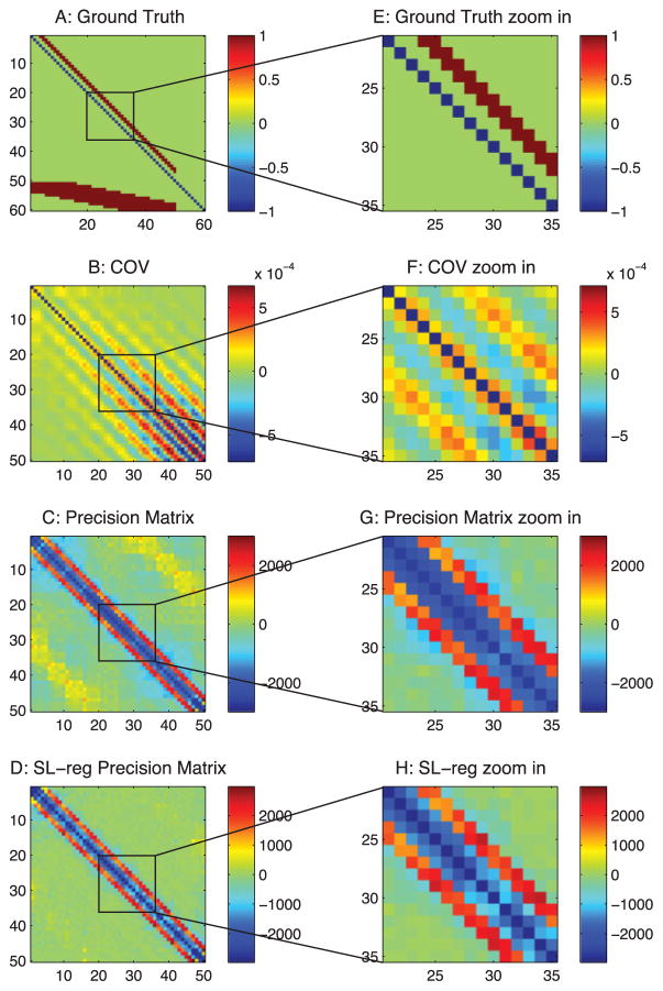
Here, we let C = 1, g_syn = 3, g_l = −5, and 𝒩_i is gaussian noise with a standard deviation of 1. The connection pattern is shown in Figure 3A. There are 60 neurons in this circuit. The first 50 neurons are connected with a pattern in which neuron i projects to neurons i + 3 and i + 4. To make the case more realistic, aside from these 50 neurons that are visible, we added 10 more neurons (neuron 51 to 60 in Figure 3A) that are invisible during our estimations (only the membrane voltages of the first 50 neurons are used to estimate connectivity). These 10 neurons send latent inputs to the visible neurons and introduce external correlations into the system. Therefore, we update our passive neuron’s model as

Figure 3.

Ground-truth connections from a passive neuron model and estimations from correlation-based methods. (A) Ground-truth connection matrix. Neurons 1 to 50 are observed neurons. Neurons 51 to 60 are unobserved neurons that introduce common inputs. (B) Estimation from the correlation method. (C) Estimation from the precision matrix. (D) Estimation from the sparse + latent regularized precision matrix. (E) Zoom-in of panel A. (F) Zoom-in of panel B. (G) Zoom-in of panel C. (H) Zoom-in of panel D.

$$C\frac{d{V}_i}{dt}=g_{\mathit{syn}}{V}_{i-4}+g_{\mathit{syn}}{V}_{i-3}+g_{\mathit{latent}}{V}_{\mathit{latent}1}+g_l{V}_i+{\mathcal{N}}_i,$$ (2.2)

where g_latent = 10. We choose the latent input’s strength in the same scale as other connections in the network. We tested multiple values between [0, 10]; higher value generates more interference and therefore makes the case more difficult.

We added the latent inputs to the system because unobserved common inputs exist in real-world problems (Stevenson et al., 2008). For example, one could be using two-photon imaging to record calcium signals from the cortical circuit. The cortical circuit might receive synaptic inputs from deeper layers in the brain, such as the thalamus, which is not visible to the microscope. Each invisible neuron projects to many visible neurons, leading to common synaptic currents to the cortical circuit, and causes neurons in the cortical circuit to be highly correlated. We will discuss how to remove interference from the latent inputs.

2.1.2 Thalamocortical Model

To test and benchmark the differential covariance-based methods in a more realistic model, we simulated neural signals from a Hodgkin-Huxley–based spiking neural network. The thalamocortical model used in this study was based on several previous studies, which were used to model spindle and slow wave activity (Bazhenov et al., 2002; Chen et al., 2012; Bonjean et al., 2011). Aschematic of the thalamocortical model in this work is shown in Figure 1. As shown, the thalamocortical model was structured as a one-dimensional, multilayer array of cells. The thalamocortical network consisted of 50 cortical pyramidal (PY) neurons, 10 cortical inhibitory (IN) neurons, 10 thalamic relay (TC) neurons, and 10 reticular (RE) neurons. The connections between the 50 PY neurons follow the pattern in the passive neuron model and are shown in Figure 7A. For the rest of the connection types, a neuron connects to all target neurons within the radius listed in Table 1 (Bazhenov et al., 2002). The network is driven by spontaneous oscillations. Details of the model are explained in appendix C.

Figure 1.

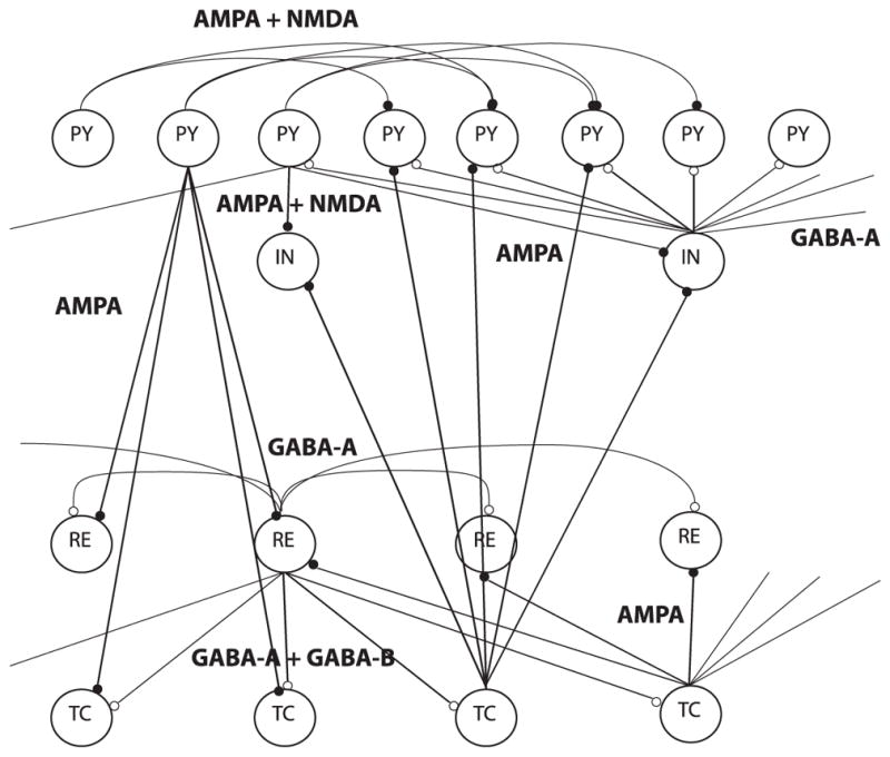
Network model for the thalamocortical interactions, with four layers of neurons: thalamocortical (TC), reticular nucleus (RE) of the thalamus, cortical pyramidal (PY), and inhibitory (IN) neurons. Filled circles indicate excitatory synapses; open circles indicate inhibitory synapses.

Figure 7.

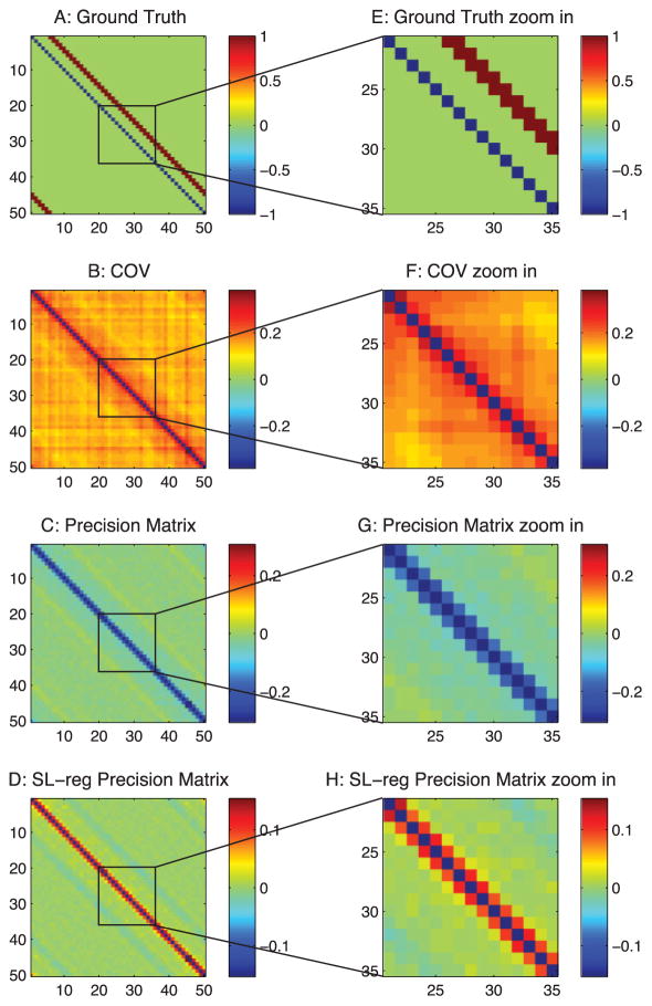
Analysis of the thalamocortical model with correlation-based methods. (A) Ground-truth connections of the PY neurons in the thalamocortical model. (B) Estimation from the correlation method. (C) Estimation from the precision matrix method. (D) Estimation from the sparse + latent regularized precision matrix method. (E) Zoom-in of panel A. (F) Zoom-in of panel B. (G) Zoom-in of panel C. (H) Zoom-in of panel D.

Table 1.

Connectivity Properties.

	PY→TC	PY→RE	TC→PY	TC→IN	PY→IN	IN→PY	RE→RE	TC→RE	RE→TC
Radius	8	6	15	3	1	5	5	8	8

For each simulation, we simulated the network for 600 secs. The data were sampled at 1000 Hz.

2.1.3 Local Field Potential (LFP) Model

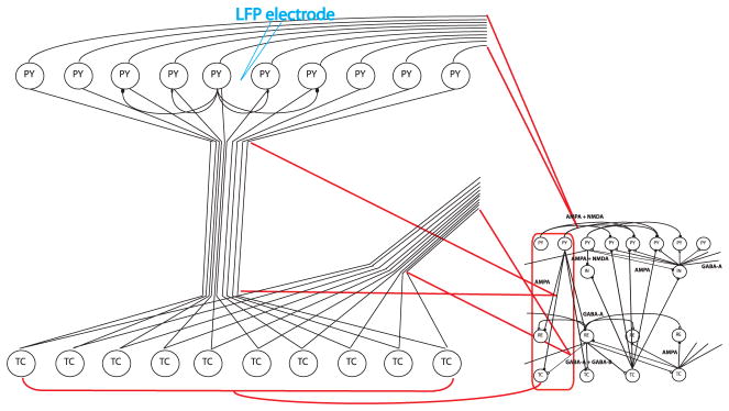
To simulate local field potential (LFP) data, we expanded the previous thalamocortical model by 10 times (see Figure 2). Each connection in the previous network (see Figure 1) is transformed into a fiber bundle connecting 10 pairs of neurons in a subnetwork. For cortical pyramidal neurons (PY), we connect each neuron to its four neighboring neurons inside the subnetwork. Other settings for the neurons and the synapses are the same as the previous thalamocortical model. We simulated the network for 600 secs. The data were sampled at 1000 Hz.

Figure 2.

The LFP model was transformed from the thalamocortical model. In this figure, we used the TC→PY connection in the red box as an example. Each neuron in the original thalamocortical model was expanded into a subnetwork of 10 neurons. Each connection in the original thalamocortical model was transformed into 10 parallel connections between two subnetworks. Moreover, subnetworks transformed from PY neurons have local connections. Each PY neuron in this subnetwork connects to its two nearest neighbors on each side. We put an LFP electrode at the center of each PY subnetwork. The electrode received neurons’ signals inversely proportional to the distance.

We plant an LFP electrode at the center of each of the 50 PY neuron local circuits. The distance between the 10 local neurons is 100 μm, and the distance between the PY subnetworks is 1 cm. The LFP is calculated according to the standard model in Bonjean et al. (2011), Destexhe (1998), and Nunez and Srinivasan (2005). The LFPs are mainly contributed by elongated dendrites of the cortical pyramidal neurons. In our model, each cortical pyramidal neuron has a 2 mm long dendrite.

For each LFP S_i,

$$S_i=\sum _j{\left(\frac{I_{\mathit{syn}}}{r_d^i}-\frac{I_{\mathit{syn}}}{r_s^i}\right)}_j,$$ (2.3)

where the sum is taken over all excitatory cortical neurons. I_syn is the postsynaptic current of neuron j, r_d is the distance from the electrode to the center of the dendrite of neuron j, and r_s is the distance from the electrode to the soma of neuron j.

2.1.4 Calcium Imaging Model

Vogelstein et al. (2009) proposed a transfer function between spike trains and calcium fluorescence signals,

$$\begin{gathered} {[Ca]}_t-{[Ca]}_{t-1}=-\frac{\mathrm{\Delta }t}{{\tau }_{Ca}}{[Ca]}_{t-1}+A_{Ca}{n}_t \\ F=\frac{[Ca]}{[Ca]+K_d}+{\eta }_t, \end{gathered}$$ (2.4)

where A_Ca = 50 μM is a step influx of calcium molecules at each action potential. n_t is the number of spikes at each time step, K_d = 300 μM is the saturation concentration of calcium, and η_t is a gaussian noise with a standard deviation of 0.000003. Since our data are sampled at 1000 Hz, we can resolve every single action potential. So in our data, there are no multiple spikes at one time step. τ_Ca = 1 s is the decay constant for calcium molecules. To maintain the information in the differential signal, instead of setting a hard cutoff value and transforming the intracellular voltages to binary spike trains, we use a sigmoid function to transform the voltages to the calcium influx activation parameter (n_t ),

$$n_t=\frac{1}{1+e^{-(V(t)-V_{\mathit{thre}})}},$$ (2.5)

where V_thre = −50 mV is the threshold potential.

In real experiments, we can image only a small percentage of neurons in the brain. Therefore, we simulated HH-based networks of 1000 neurons and record from only 50 neurons. We used the four connection patterns (normal-1 ~ normal-4) provided online (https://www.kaggle.com/c/connectomics) (Stetter, Battaglia, Soriano, & Geisel, 2012). Briefly, the networks have 80% excitatory neurons and 20% inhibitory neurons. The connection probability is 0.01—one neuron connects to about 10 neurons— so it is a sparsely connected network.

Similar to our thalamocortical model, we used AMPA and NMDA synapses for the excitatory synapses and GABA synapses for the inhibitory synapses. The simulations ran 600 sec and were sampled at 1000 Hz. The intracellular voltages obtained from the simulations were then transferred to calcium fluorescence signals and downsampled to 50 Hz. For each of the four networks, we conducted 25 recordings. Each recording contains calcium signals from 50 randomly selected neurons.

For accurate estimations, the differential covariance-based methods require the reconstructed action potentials from the calcium imaging. While this is an active research area and many methods have been proposed (Quan, Liu, Lv, Chen, & Zeng, 2010; Rahmati, Kirmse, Marković, Holthoff, & Kiebel, 2016), in this study, we simply reversed the transfer function. By assuming the transfer function from action potentials to calcium fluorescence signals is known, we can reconstruct the action potentials. Given F̂ as the observed fluorescence signal,

$$\begin{gathered} [\widehat{C}a]=\widehat{F}\ast K_d/(1-\widehat{F}) \\ {\widehat{n}}_t=(d[\widehat{C}a]+1/{\tau }_{Ca}{[Ca]}_t)/(A/\mathrm{\Delta }t) \\ \widehat{V}=log(1/n_t-1). \end{gathered}$$ (2.6)

2.2 Differential Covariance-Based Methods

In this section, we introduce a new class of methods to estimate the functional connectivity of neurons (code is provided online at https://github.com/tigerwlin/diffCov).

2.2.1 Step 1: Differential Covariance

The input to the method, V(t), is an N × T neural recording data set. N is the number of neurons or channels recorded, and T is the number of data samples during recordings. We compute the derivative of each time series with dV(t) = (V(t + 1) −V(t − 1))/(2dt). Then the covariance between V(t) and dV(t) is computed and denoted as Δ_C, which is an N × N matrix defined as

$${\mathrm{\Delta }}_{C_{i,j}}=cov(d{V}_i(t),V_j(t)),$$ (2.7)

where dV_i(t) is the differential signal of neuron/channel i, V_j (t) is the signal of neuron/channel j, and cov() is the sample covariance function for two time series. In appendix A, we provide a theoretical proof about why the differential covariance estimator generates fewer false connections than the covariance-based methods do.

2.2.2 Step 2: Applying Partial Covariance Method

As Stevenson et al. (2008) previously mentioned, one problem of the correlation method is the propagation of correlation. Here we designed a customized partial covariance algorithm to reduce this type of error in our methods. We use Δ_{Pi, j} to denote the differential covariance estimation after applying the partial covariance method.

Using the derivation from section B.2, we have

$${\mathrm{\Delta }}_{P_{i,j}}={\mathrm{\Delta }}_{C_{i,j}}-{\text{COV}}_{j,z}·{\text{COV}}_{Z,Z}^{-1}·{\mathrm{\Delta }}_{C_{i,Z}}^T,$$ (2.8)

where Z is a set of all neurons/channels except {i, j}:

$$Z=\{1,2,\dots ,i-1,i+1,\dots ,j-1,j+1,\dots N\}.$$

Δ_{Ci, j} and Δ_Ci,Z were computed from section 2.2.1, and COV_Z,Z is the covariance matrix of set Z. COV_j,Z is a flat matrix denoting the covariance of neuron j and neurons in set Z. · is the matrix dot product.

As we explain in section B.2, the partial covariance of the differential covariance is not equivalent to the inverse of the differential covariance estimation. The two are equivalent only for the covariance matrix and when the partial correlation is controlling on all variables in the observed set. In our case, the differential covariance matrix is nonsymmetric because it is the covariance between recorded signals and their differential signals. We have signals and differential signals in our observed set; however, we are controlling only on the original signals for the partial covariance algorithm. Due to these differences, we developed this customized partial covariance algorithm, equation 2.8, which performs well for neural signals in the form of equation 2.2.

2.2.3 Step 3: Sparse Latent Regularization

Finally, we applied the sparse latent regularization method to partial covariance version of the differential covariance (Chandrasekaran, Sanghavi, Parrilo, & Willsky, 2011; Yatsenko et al., 2015). As explained in section B.3, in the sparse latent regularization method, we made the assumption that there are observed neurons and unobserved common inputs in a network. If the connections between the observed neurons are sparse and the number of unobserved common inputs is small, this method can separate the covariance into two parts and the sparse matrix is the intrinsic connections between the observed neurons.

Here we define Δ_S as the sparse result from the method and L as the low-rank result from the method. Then we solve arg min

$$\underset{{\mathrm{\Delta }}_S,L}{argmin}{\left|\right|{\mathrm{\Delta }}_S\left|\right|}_1+\alpha \ast tr(L)$$ (2.9)

under the constraint that

$${\mathrm{\Delta }}_P={\mathrm{\Delta }}_S+L,$$ (2.10)

where || ||₁ is the L1-norm of a matrix and tr() is the trace of a matrix. α is the penalty ratio between the L1-norm of Δ_S and the trace of L. It was set to $1/\sqrt{N}$ for all our estimations. Δ_P is the partial differential covariance computed from section 2.2.2. We receive a sparse estimation, Δ_S, of the connectivity.

2.2.4 Computing Derivative

In differential covariance, computing the derivative using dV(t) = (V(t + 1) −V(t − 1))/(2dt) provides better estimation results than using dV(t + 1) = (V(t + 1) −V(t))/dt. To elaborate this point, we first explain our method’s connection to the autoregressive (AR) method.

Detailed discussion of the multivariate autoregressive model and its estimators has been discussed in Harrison et al. (2003). In discrete space, our differential covariance estimator is similar to the mean squared error (MSE) estimator of the AR model. Following the definition in equation 2.2, we have

$$C\frac{dV(t)}{dt}=G·V(t)+\mathcal{N},$$ (2.11)

where V(t) are neurons’ membrane voltages. G is the connection matrix that describes the conductance between each pair of neurons. 𝒩 is the gaussian noise.

For dV(t) = (V(t + 1) −V(t − 1))/(2dt), we note here:

$$\begin{gathered} C\frac{dV(t)}{dt}=C\frac{V(t+1)-V(t-1)}{2\mathrm{\Delta }t}=G·V(t)+\mathcal{N}, \\ V(t+1)=\frac{2\mathrm{\Delta }t}{C}G·V(t)+V(t-1)+\frac{2\mathrm{\Delta }t}{C}\mathcal{N}. \end{gathered}$$ (2.12)

As Harrison et al. (2003) explained, in the AR model, the MSE estimator of G is $\frac{(V(t+1)-V(t-1))V{(t)}^T}{V(t)V{(t)}^T}$. We note that the numerator of this MSE estimator is our differential covariance estimator. Therefore, in this case, the model we proposed is equivalent to a regularized AR(2) model, where the transition matrix of the second order is restricted to be an identity matrix.

In the dV(t) = (V(t + 1) −V(t))/dt case, we note that the differential covariance estimator is similar to an AR(1) estimator,

$$\begin{gathered} C\frac{dV(t)}{dt}=C\frac{V(t+1)-V(t)}{\mathrm{\Delta }t}=G·V(t)+\mathcal{N}, \\ V(t+1)=\left(\frac{\mathrm{\Delta }t}{C}G+I\right)·V(t)+\frac{\mathrm{\Delta }t}{C}\mathcal{N}, \end{gathered}$$ (2.13)

and the MSE estimator of $\left(\frac{\mathrm{\Delta }t}{C}G+I\right)$ is $\frac{V(t+1)V{(t)}^T}{V(t)V{(t)}^T}$. Therefore:

$$\begin{gathered} \frac{\mathrm{\Delta }t}{C}G=\frac{V(t+1)V{(t)}^T}{V(t)V{(t)}^T}-I \\ =\frac{(V(t+1)-V(t))V{(t)}^T}{V(t)V{(t)}^T}, \end{gathered}$$ (2.14)

where the numerator of this MSE estimator is our differential covariance estimator.

As explained above, using different methods to compute the derivative will produce different differential covariance estimators, and they are equivalent to estimators from different AR models for the connection matrix. In section 3, we show that the performances of these two estimators are significantly different.

2.3 Performance Quantification

The performance of each method is judged by four quantified values. The first three values indicate the method’s abilities to reduce the three types of false connections (see Figure 4). The last one indicates the method’s ability to correctly estimate the true positive connections against all possible interference.

Figure 4.

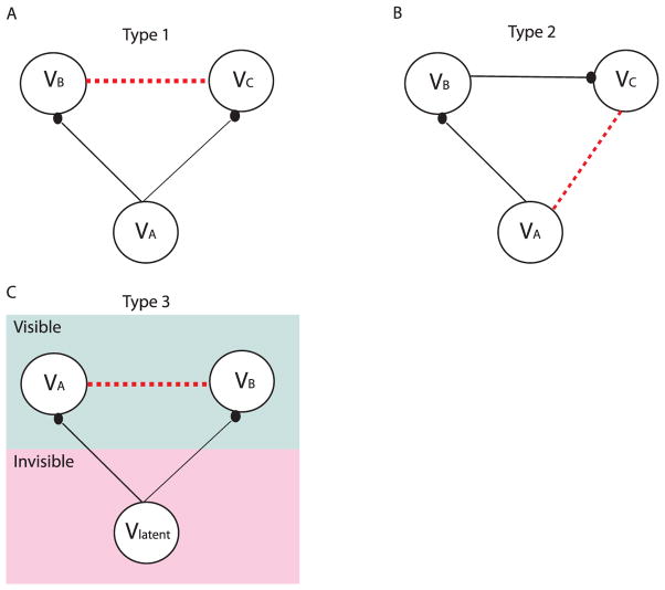
Illustrations of the three types of false connections in the correlation-based methods. Solid lines indicate the physical wiring between neurons, and the filled circles at the end indicate the synaptic contacts (i.e., the direction of the connections). The dotted lines are the false connections introduced by the correlation-based methods. (A) Type 1 false connections, which are due to two neurons receiving the same synaptic inputs. (B) Type 2 false connections, which are due to the propagation of correlation. (C) Type 3 false connections, which are due to unobserved common inputs.

We define G as the ground-truth connectivity matrix, where:

$$G_{i,j}=\{\begin{array}{ll}1,\hfill & \text{if}\text{neuron}i\text{projects}\text{to}\text{neuron}j\text{with}\text{excitatory}\text{synapse}\hfill \\ -1,\hfill & \text{if}\text{neuron}i\text{projects}\text{to}\text{neuron}j\text{with}\text{inhibitory}\text{synapse}.\hfill \\ 0,\hfill & \text{otherwise}\hfill \end{array}$$ (2.15)

Then we can use a three-dimensional tensor to represent the false connections caused by common inputs. For example, neurons j and k receive common input from neuron i:

$$M_{i,j,k}=\{\begin{array}{ll}1,\hfill & \text{iff}{G}_{i,j}=1\text{and}{G}_{i,k}=1\hfill \\ 0,\hfill & \text{otherwise}\hfill \end{array}.$$ (2.16)

Therefore, we can compute a mask that labels all of the type 1 false connections:

$${\mathit{mask}}_{1_{j,k}}=\sum _{i\in \left\{\text{observed}\text{neurons}\right\}}{M}_{i,j,k}.$$ (2.17)

For the type 2 false connections (e.g., neuron i projects to neuron k; then neuron k projects to neuron j), the mask is defined as

$${\mathit{mask}}_{2_{i,j}}=\sum _{k\in \left\{\text{observed}\text{neurons}\right\}}{G}_{i,k}{G}_{k,j}$$ (2.18)

or, in simple matrix notation,

$${\mathit{mask}}_2=G·G.$$ (2.19)

Similar to mask₁, the false connections caused by unobserved common inputs are

$${\mathit{mask}}_{3_{j,k}}=\sum _{i\in \left\{\text{unobserved}\text{neurons}\right\}}{M}_{i,j,k}.$$ (2.20)

Finally, mask₄ is defined as

$${\mathit{mask}}_{4_{i,j}}=\{\begin{array}{ll}1,\hfill & \text{if}{G}_{i,j}=0\hfill \\ 0,\hfill & \text{otherwise}\hfill \end{array}.$$ (2.21)

Given a connectivity matrix estimation result, Est, the four values for the performance quantification are computed as the area under the ROC curve for two sets: the true positive set and the false positive set:

$$\begin{gathered} \mid {\mathit{Est}}_{i,j}\mid \in {\left\{\text{true}\text{positive}\text{set}\right\}}_k,\text{if}{G}_{i,j}\ne 0\text{and}{\mathit{mask}}_{k_{i,j}}=0, \\ \mid {\mathit{Est}}_{i,j}\mid \in {\left\{\text{false}\text{positive}\text{set}\right\}}_k,\text{if}{\mathit{mask}}_{k_{i,j}}\ne 0\text{and}{G}_{i,j}=0. \end{gathered}$$ (2.22)

3 Results

3.1 False Connections in Correlation-Based Methods

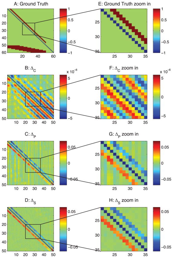
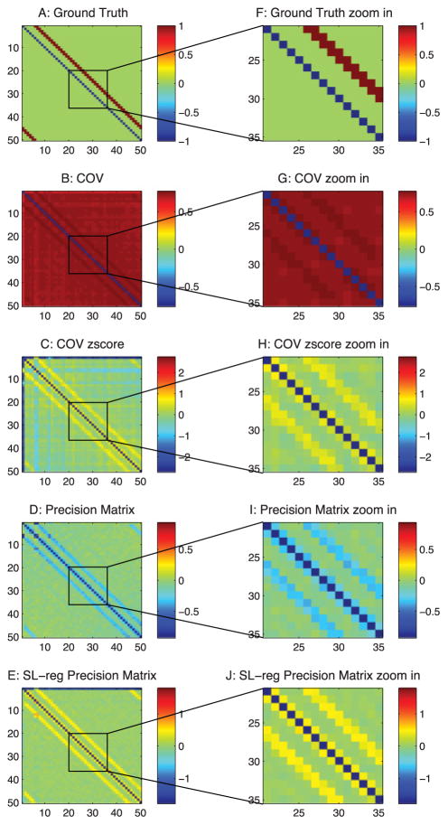
When applied to neural circuits, the commonly used correlation-based methods produce systematic false connections. As shown, Figure 3A is the ground truth of the connections in our passive neuron model (neurons 1 to 50 are the observed neurons). Figure 3B is from the correlation method, Figure 3C is the precision matrix, and Figure 3D is the sparse + latent regularized precision matrix. As shown, all of these methods produce extra false connections.

For convenience of explanation, we define the diagonal strip of connections in the ground truth (the first 50 neurons in Figure 3A) as the −3 and −4 diagonal lines, because they are three and four steps away from the diagonal line of the matrix. As shown in Figure 3, all of these methods produce false connections on the ±1 diagonal lines. The precision matrix method (see Figure 3C) also has square box shape of false connections in the background.

3.1.1 Type 1 False Connections

The type 1 false connections shown in Figure 4A are produced because two neurons receive the same input from another neuron. The same synaptic current that passes into the two neurons generates a positive correlation between the two neurons. However, there is no physiological connection between these two neurons. In our connection pattern (see Figure 3A), we notice that two neurons next to each other receive common synaptic inputs; therefore, there are false connections on the ±1 diagonal lines of the correlation-based estimations.

3.1.2 Type 2 False Connections

The type 2 false connections shown in Figure 4B are due to the propagation of correlation. Because one neuron V_A connects to another neuron V_B and neuron V_B connects to another neuron V_C, the correlation method presents the correlation between V_A and V_C, which do not have a physical connection. This phenomenon is shown in Figure 3B as the extra diagonal strips. This problem, shown in Figure 3C can be greatly reduced by the precision matrix/partial covariance method.

3.1.3 Type 3 False Connections

The type 3 false connections shown in Figure 4C are also due to the common currents that pass into two neurons. However, in this case, they are from the unobserved neurons. For this particular passive neuron model, it is due to the inputs from the 10 unobserved neurons (neurons 51–60) as shown in Figure 3A. Because the latent neurons have broad connections to the observed neurons, they introduce a square box shape correlation pattern into the estimations. (See Figure 3C. Figure 3B also contains this error, but it is hard to see.) Since the latent neurons are not observable, the partial covariance method cannot be used to regress out this type of correlation. The sparse latent regularization can be applied if the sparse and low-rank assumption is valid, and the sparse + latent regularized result is shown in Figure 3D. However, even after using this regularization, the correlation-based methods still leave false connections in Figure 3D.

3.2 Estimations from Differential Covariance-Based Methods

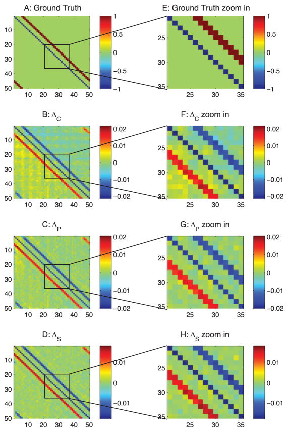
Comparing the ground-truth connections in Figure 5A with our final estimation in Figure 5D, we see that our methods essentially transformed the connections in the ground truth into a map of sources and sinks in a network. An excitatory connection, i → j, in our estimations has a negative value for Δ_{Si j} and a positive value for Δ_Sji, which means the current is coming out of the source i and goes into the sink j. We note that there is another ambiguous case, an inhibitory connection j → i, which produces the same results in our estimations. Our methods cannot differentiate these two cases; instead, they indicate sources and sinks in a network.

Figure 5.

Differential covariance analysis of the passive neuron model. The color in panels B, C, D, F, G, and H indicate the direction of the connections. For element A_{i j}, a warm color indicates i is the sink and j is the source—that is, i ← j—and the cool color indicates j is the sink and i is the source—that is, i → j. (A) Ground-truth connection matrix. (B) Estimation from the differential covariance method. (C) Estimation from the partial differential covariance method. (D) Estimation from the sparse + latent regularized partial differential covariance method. (E) Zoom-in of panel A. (F) Zoom-in of panel B. (G) Zoom-in of panel C. (H) Zoom-in of panel D.

3.2.1 The Differential Covariance Method Reduces Type 1 False Connections

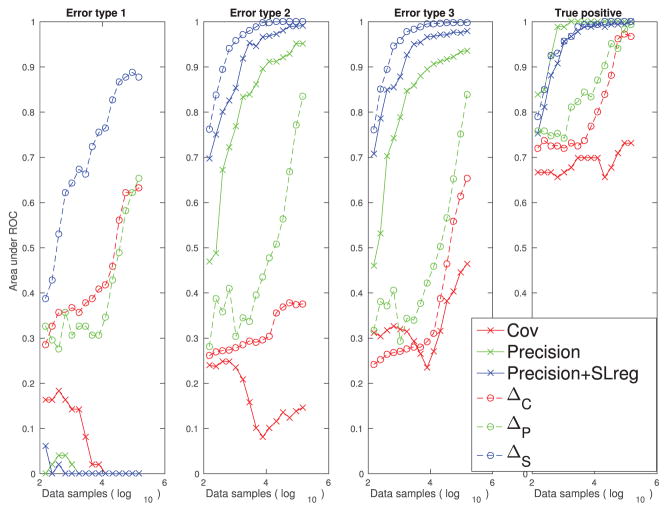
By comparing Figure 3B with Figure 5B, we see that the type 1 false connections on the ±1 diagonal lines of Figure 3B are reduced in Figure 5B. This is reflecting the theorems we prove in appendix A, in particular theorem 5, which shows that the strength of the type 1 false connections is reduced in the differential covariance method by a factor of g_l/g_syn. Moreover, the performance of the differential covariance method on reducing type 1 false connections is quantified in Figure 6.

Figure 6.

Performance quantification (area under the ROC curve) of different methods with respect to their abilities to reduce the three types of false connections and their abilities to estimate the true positive connections using the passive neuron data set.

3.2.2 The Partial Covariance Method Reduces Type 2 False Connections

Second, we see that due to the propagation of correlation, there are extra diagonal strips in Figure 5B. These are removed in Figure 5C by applying the partial covariance method. Each estimator’s performance for reducing type 2 false connections is quantified in Figure 6.

3.2.3 The Sparse + Latent Regularization Reduces Type 3 False Connections

Third, the sparse + latent regularization to remove the correlation is introduced by the latent inputs. When the observed neurons’ connections are sparse and the number of unobserved common inputs is small, the covariance introduced by the unobserved common inputs can be removed. As shown in Figure 5D, the external covariance in the background of Figure 5C is removed, while the true diagonal connections and the directionality of the connections are maintained. This regularization is also effective for correlation-based methods, but type 1 false connections are maintained in the estimation even after applying this regularization (see Figure 3D). Each estimator’s performance for reducing type 3 false connections is quantified in Figure 6.

3.2.4 The Differential Covariance-Based Methods Provide Directionality Information of the Connections

Using this passive neuron model, in section A.3, we provide a mathematical explanation for why the differential covariance-based methods provide directional information for the connections. Given an excitatory connection g_i→j (neuron i projects to neuron j), from theorem 6 in section A.3, we have

$$\begin{gathered} {\mathrm{\Delta }}_{C_{j,i}}>0, \\ {\mathrm{\Delta }}_{C_{i,j}}<0. \end{gathered}$$ (3.1)

We note here that there is another ambiguous setting that provides the same result, which is an inhibitory connection g_j→i. Conceptually, the differential covariance indicates the current sources and sinks in a neural circuit, but the exact type of synapse is unknown.

3.2.5 Performance Quantification for the Passive Neuron Data Set

In Figure 6, we quantified the performance of the estimators for one example data set. We see that with the increase in the sample size, our differential covariance-based methods reduce the three types of false connections, while maintaining high true positive rates. Also, as we apply more advanced techniques (Δ_C → Δ_P → Δ_S), the estimator’s performance increases in all four panels of the quantification indices. Although the precision matrix and the sparse + latent regularization help the correlation method reduce type 2 and type 3 errors, all correlation-based methods handle the type 1 false connections poorly. We also note that the masks we used to quantify each type of false connections are not mutually exclusive (i.e., there are false connections that belong to more than one type of false connections). Therefore, in Figure 6, it seems that a regularization is reducing the multiple types of false connections. For example, the sparse + latent regularization is reducing both type 2 and type 3 false connections.

In Table 2, we provide quantified results (area under the ROC curve) for two connection patterns (cxcx34, and cxcx56789) and three conductance settings (g5, g30, and g50). We see that the key results in Figure 6 are also generalized here. By applying more advanced techniques to the original differential covariance estimator (Δ_C → Δ_P → Δ_S), the performance increases with respect to the three types of error, while the true positive rate is not sacrificed. We also note that although the precision matrix and the sparse + latent regularization help the correlation method reduce type 2 and type 3 errors, all correlation-based methods handle the type 1 error poorly.

Table 2.

Performance Quantification (Area under the ROC Curve) of Different Methods with Respect to Their Abilities to Reduce the Three Types of False Connections and Their Abilities to Estimate the True Positive Connections under Five Different Passive Neuron Model Settings.

	Cov	Precision	Precision+SL-reg	ΔC	ΔP	ΔS
cxcx34 g5
Error 1	0	0	0	0.6327	0.3469	0.8776
Error 2	0.1469	0.9520	0.9915	0.3757	0.8347	1.0000
Error 3	0.4638	0.9362	0.9797	0.6541	0.8391	0.9986
True positive	0.7312	1.0000	1.0000	0.9677	0.9946	1.0000
cxcx34 g30
Error 1	0	0	0	0.0510	0.5816	0.9490
Error 2	0.0056	0.8927	0.9972	0.2881	0.9548	1.0000
Error 3	0.2164	0.9188	0.9942	0.5430	0.9662	1.0000
True positive	0.5591	1.0000	0.9892	0.6559	1.0000	1.0000
cxcx34 g50
Error 1	0	0	0	0	0.2041	0.6531
Error 2	0	0.7034	0.9944	0.0523	0.9054	1.0000
Error 3	0.3179	0.8000	0.9894	0.4145	0.9309	1.0000
True positive	0.9140	1.0000	0.9946	0.9516	0.9785	1.0000
cxcx56789 g5
Error 1	0	0.0053	0.0053	0.6895	0.6263	0.8526
Error 2	0.1896	0.6229	0.7896	0.5240	0.7896	0.9938
Error 3	0.3573	0.6085	0.7659	0.6957	0.7591	0.9817
True positive	0.6884	0.9442	0.6674	0.9930	0.9605	0.9837
cxcx56789 g50
Error 1	0	0	0	0.0263	0.2816	0.6842
Error 2	0.1083	0.5312	0.8240	0.2844	0.6990	0.9979
Error 3	0.4256	0.4927	0.7762	0.5091	0.7116	0.9835
True positive	0.9256	0.9116	0.6698	0.9395	0.9279	0.9419

3.3 Thalamocortical Model Results

We tested the methods further in a more realistic Hodgkin-Huxley–based model. Because the synaptic conductances in the model are no longer constants but become nonlinear dynamic functions, which depend on the presynaptic voltages, the previous derivations can be considered only a first-order approximation.

The ground-truth connections between the cortical neurons are shown in Figure 7. These neurons also receive latent inputs from and send feedback currents to inhibitory neurons in the cortex (IN) and thalamic neurons (TC). For clarity of representation, these latent connections are not shown here; the detailed connections are described in section 2.

Similar to the passive neuron model, in Figure 7B, the correlation method still suffers from those three types of false connections. As shown, the latent inputs generate false correlations in the background, and the ±1 diagonal line false connections, which are due to the common currents, exist in all correlation-based methods (see Figures 7B–7D). Comparing Figures 7C and 7D because the type 1 false connections are strong in the Hodgkin- Huxley–based model, the sparse + latent regularization removed the true connections but kept these false connections in its final estimation.

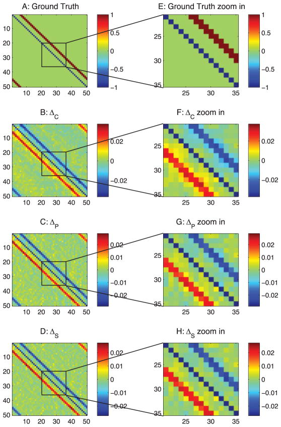
As shown in Figure 8B, differential covariance method reduces the type 1 false connections. In Figure 8C, the partial differential covariance method reduces type 2 false connections in Figure 8B (the yellow connections around the red strip in Figure 8B). Finally, in Figure 8D, the sparse latent regularization removes the external covariance in the background of Figure 8C. The current sources (positive value, red) and current sinks (negative value, blue) in the network are also indicated on our estimators.

Figure 8.

Analysis of the thalamocortical model with differential covariance-based methods. The color in panels B, C, D, F, G, and H indicates the direction of the connections. For element A_{i j}, a warm color indicates i is the sink and j is the source—i ← j. A cool color indicates j is the sink and i is the source—i → j. (A) Ground-truth connection matrix. (B) Estimation from the differential covariance method. (C) Estimation from the partial differential covariance method. (D) Estimation from the sparse + latent regularized partial differential covariance method. (E) Zoom-in of panel A. (F) Zoom-in of panel B. (G) Zoom-in of panel C. (H) Zoom-in of panel D.

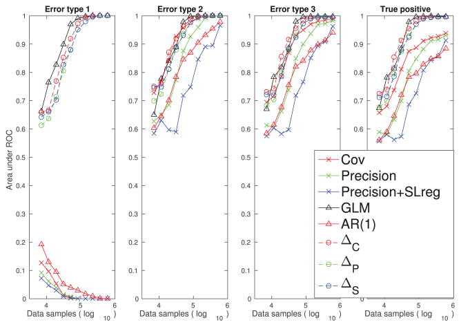
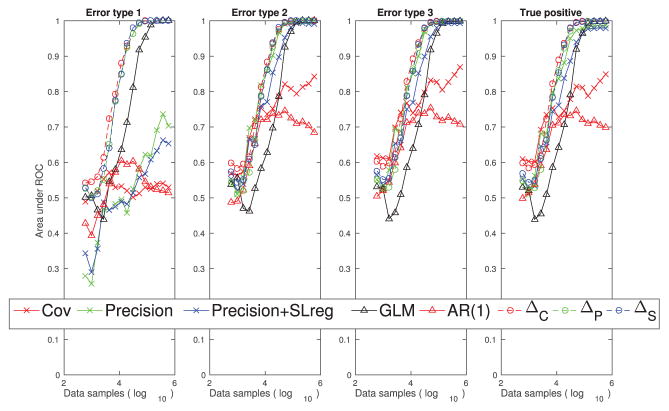
In Figure 9, each estimator’s performance on each type of false connections is quantified. In this example, our differential covariance-based methods achieve similar performance to the GLM method.

Figure 9.

Performance quantification (area under the ROC curve) of different methods with respect to their abilities to reduce the three types of false connections and their abilities to estimate the true positive connections using the thalamocortical data set.

3.4 Simulated LFP Results

For population recordings, our methods have similar performance to the thalamocortical model example. While the correlation-based methods are still suffering from the problem of type 1 false connections (see Figure 10), our differential covariance-based methods can reduce all three types of false connections (see Figure 11). In Figure 12, each estimator’s performance on LFP data is quantified. In this example, with sufficient data samples, our differential covariance-based methods achieve performance similar to that of the GLM method. For smaller sample sizes, our new methods perform better than the GLM method.

Figure 10.

Analysis of the simulated LFP data with correlation-based methods. (A) Ground-truth connection matrix. (B) Estimation from the correlation method. (C) z-score of the correlation matrix. (D) Estimation from the precision matrix method. (E) Estimation from the sparse + latent regularized precision matrix method. (F) Zoom-in of panel A. (G) Zoom-in of panel B. (H) Zoom-in of panel C. (I) Zoom-in of panel D. (J) Zoom-in of panel E.

Figure 11.

Analysis of the simulated LFP data with differential covariance-based methods. The color in panels B, C, D, F, G, and H indicates the direction of the connections. For element A_{i j}, a warm color indicates i is the sink and j is the source—i ← j. A cool color indicates j is the sink and i is the source—i → j. (A) Ground-truth connection matrix. (B) Estimation from the differential covariance method. (C) Estimation from the partial differential covariance method. (D) Estimation from the sparse + latent regularized partial differential covariance method. (E) Zoom-in of panel A. (F) Zoom-in of panel B. (G) Zoom-in of panel C. (H) Zoom-in of panel D.

Figure 12.

Performance quantification (area under the ROC curve) of different methods with respect to their abilities to reduce the three types of false connections and their abilities to estimate the true positive connections using the simulated LFP data set.

3.5 Simulated Calcium Imaging Results

Because current techniques allow recording of only a small percentage of neurons in the brain, we tested our methods on a calcium imaging data set of 50 neurons recorded from networks of 1000 neurons. In this example, our differential covariance-based methods (see Figure 14) match better with the ground truth than the correlation-based methods (see Figure 13).

Figure 14.

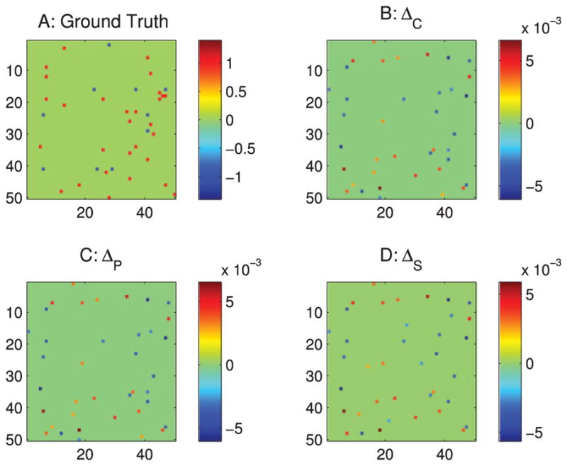
Analysis of the simulated calcium imaging data set with differential covariance-based methods. The color in panels B–D indicates the direction of the connections. For element A_{i j}, a warm color indicates i is the sink and j is the source—i ← j. A cool color indicates j is the sink and i is the source—i → j. (A) Ground truth connection matrix. (B) Estimation from the differential covariance method. (C) Estimation from the partial differential covariance method. (D) Estimation from the sparse + latent regularized partial differential covariance method. For clarity, panels B, C, and D are thresholded to show only the strongest connections, so one can compare it with the ground truth.

Figure 13.

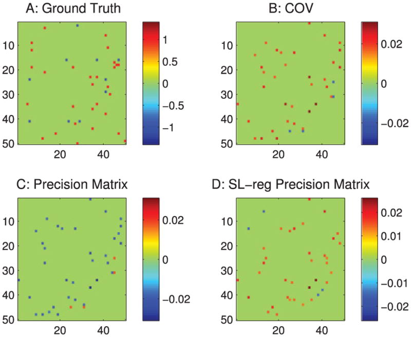
Analysis of the simulated calcium imaging data set with correlation-based methods. (A) Ground-truth connection matrix. (B) Estimation from the correlation method. (C) Estimation from the precision matrix method. (D) Estimation from the sparse + latent regularized precision matrix method. For clarity, panels B, C, and D are thresholded to show only the strongest connections, so one can compare it with the ground truth.

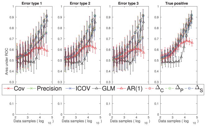
We performed 25 sets of recordings with 50 neurons randomly selected in each of the four large networks and quantified the results. The markers on the plots in Figure 15 are the average area under the ROC curve values across the 100 sets, and the error bars indicate the standard deviations across these 100 sets of recordings. Our differential covariance-based methods perform better than the GLM method, and the performance differences seem to be greater in situations with fewer data samples.

4 Discussion

4.1 Generalizability and Applicability of the Differential Covariance-Based Methods to Real Experimental Data

Many methods have been proposed to solve the problem of reconstructing the connectivity of a neural network. Winterhalder et al. (2005) reviewed the nonparametric methods and Granger causality–based methods. Much progress has been made recently using the kinetic Ising model and Hopfield network (Huang, 2013; Dunn & Roudi, 2013; Battistin, Hertz, Tyrcha, & Roudi, 2015; Capone, Filosa, Gigante, Ricci-Tersenghi, & Del Giudice, 2015; Roudi & Hertz, 2011) with sparsity regularization (Pernice & Rotter, 2013). The GLM method (Okatan et al., 2005; Truccolo et al., 2005; Pillow et al., 2008) and the maximum entropy method (Schneidman, Berry, Segev, & Bialek, 2006) are two popular classes of methods and the main modern approaches for modeling multiunit recordings (Roudi, Dunn, & Hertz, 2015).

In current research, people are recording more and more neurons and looking for new data analysis techniques to handle bigger data with higher dimensionality. The field is in favor of algorithms that require fewer samples and scale well with dimensionality, but without sacrificing accuracy. Also, an algorithm that is model free or makes minimum assumptions about the hidden structure of the data has the potential to be applied to multiple types of neural recordings.

The key difference between our methods and other ones is that we use the relationship between a neuron’s differential voltage and its voltage rather than finding the relationship between voltages. This provides better performance because the differential voltage is a proxy for a neuron’s synaptic current. Also, the relationship between a neuron’s synaptic current and its input voltages is more linear, which is suitable for data analysis techniques like the covariance method. While this linear relationship holds only for our passive neuron model, we still see similar or better performance of our methods in our examples based on the Hodgkin-Huxley model, where we relaxed this assumption and allowed loops in the networks. This implies that this class of methods is still applicable even when the ion channels’ conductances vary nonlinearly with the voltages, which makes the linear relationship hold only weakly.

4.2 Caveats and Future Directions

One open question for the differential covariance-based methods is how to improve the way they handle neural signals that are nonlinearly transformed from the intracellular voltages. Currently, to achieve good performance in the calcium imaging example, we need to assume we know the exact transfer function and reversely reconstruct the action potentials. We find this reverse transform method to be prone to additive gaussian noise. Further study is needed to find a better way to preprocess calcium imaging data for the differential covariance–based methods.

Throughout our simulations, the differential covariance method has better performance and needs fewer data samples in some simulations but not in others. Further investigation is needed to understand where the improvement comes from.

Our Hodgkin-Huxley simulations did not include axonal or synaptic delays, a critical feature of a real neural circuit. Unfortunately, it is nontrivial to add this feature to our Hodgkin-Huxley model. Nevertheless, we tested our methods with the passive neuron model using the same connection patterns but with random synaptic delays between neurons. In appendix D, we show that for up to a 10 ms uniformly distributed synaptic delay pattern, our methods still outperform the correlation-based methods.

Appendix A: Differential Covariance Derivations

In this appendix we first build a simple three-neuron network to demonstrate that our differential covariance–based methods can reduce type 1 false connections. Then we develop a generalized theory showing that the type 1 false connections’ strength is always lower in our differential covariance–based methods than the original correlation-based methods.

Figure 15.

Performance quantification (area under the ROC curve) of different methods with respect to their abilities to reduce the three types of false connections and their abilities to estimate the true positive connections using the simulated calcium imaging data set. The error bar is the standard deviation across 100 sets of experiments. Each experiment randomly recorded 50 neurons in a large network. The markers on the plots indicate the average area under the ROC curve values across the 100 sets of experiments.

A.1 A Three-Neuron Network

Let us assume a network of three neurons, where neuron A projects to neurons B and C:

$$\begin{gathered} I_A=d{V}_A/dt=g_l{V}_A+{\mathcal{N}}_A, \\ {I}_B=d{V}_B/dt=g_1{V}_A+g_l{V}_B+{\mathcal{N}}_B, \\ {I}_C=d{V}_C/dt=g_2{V}_A+g_l{V}_C+{\mathcal{N}}_C. \end{gathered}$$ (A.1)

Here, the cell conductance is g_l, neuron A’s synaptic connection strength to neuron B is g₁, and neuron A’s synaptic connection strength to neuron C is g₂. 𝒩_A, 𝒩_B, 𝒩_C are independent white gaussian noises.

From equation 18 of Fan, Shan, Yuan, and Ren (2011), we can derive the covariance matrix of this network:

$$\mathit{vec}(\text{COV})=-{(G\otimes I_n+I_n\otimes G)}^{-1}(D\otimes D)\mathit{vec}(I_m),$$ (A.2)

where

$$G={\left[\begin{array}{ccc}{g}_l& g_1& g_2\\ 0& g_l& 0\\ 0& 0& g_l\end{array}\right]}^T$$ (A.3)

is the transpose of the ground-truth connection of the network. And

$$D=\left[\begin{array}{ccc}1& 0& 0\\ 0& 1& 0\\ 0& 0& 1\end{array}\right]$$ (A.4)

since each neuron receives independent noise. I_n is an identity matrix of the size of G, and I_m is an identity matrix of the size of D. ⊗ is the Kronecker product, and vec() is the column vectorization function.

Therefore, we have the covariance matrix of the network as:

$$\text{COV}=\left[\begin{array}{ccc}-1/(2\ast g_l)& g_1/(4\ast g_l^2)& g_2/(4\ast g_l^2)\\ g_1/(4\ast g_l^2)& -(g_1^2+2\ast g_l^2)/(4\ast g_l^3)& -(g_1\ast g_2)/(4\ast g_l^3)\\ g_2/(4\ast g_l^2)& -(g_1\ast g_2)/(4\ast g_l^3)& -(g_2^2+2\ast g_l^2)/(4\ast g_l^3)\end{array}\right].$$ (A.5)

When computing the differential covariance, we plug in equation A.1—for example:

$$\text{COV}(I_C,V_B)=g_2\text{COV}(V_A,V_B)+g_l\text{COV}(V_C,V_B).$$ (A.6)

Therefore, from equation A.5, we can compute the differential covariance as

$${\mathrm{\Delta }}_P=\left[\begin{array}{ccc}-1/2& g_1/(4\ast g_l)& g_2/(4\ast g_l)\\ -g_1/(4\ast g_l)& -1/2& 0\\ -g_2/(4\ast g_l)& 0& -1/2\end{array}\right].$$ (A.7)

Notice that because the ratio between COV(V_A, V_B) and COV(V_C, V_B) is –g_l/g₂, in differential covariance, the type 1 false connection COV(I_C, V_B) has value 0.

A.2 Type 1 False Connection’s Strength Is Reduced in Differential Covariance

In this section, we propose a theory. A network consists of passive neurons in the following form,

$$I_i(t)=C\frac{d{V}_i(t)}{dt}=\sum _{k\in \{{\mathit{pre}}_i\}}{g}_{k\to i}{V}_k(t)+g_l{V}_i(t)+d{B}_i(t),$$ (A.8)

where {pre_i} is the set of neurons that project to neuron i, g_k→i is the synaptic conductance for the projection from neuron k to neuron i, and B_i(t) is a Brownian motion. Further assume that:

• All neurons’ leakage conductance g_l and membrane capacitance C are constants and the same.

• There is no loop in the network.

• g_syn ≪ g_l, where g_syn is the maximum of |g_i→j|, for ∀i, j

Then we prove below that:

• For two neurons that have physical connection, their covariance is $O\left(\frac{g_{\mathit{syn}}}{g_l^2}\right)$.

• For two neurons that do not have physical connection, their covariance is $O\left(\frac{g_{\mathit{syn}}^2}{g_l^3}\right)$.

• For two neurons that have physical connection, their differential covariance is $O\left(\frac{g_{\mathit{syn}}}{g_l}\right)$.

• For two neurons that do not have physical connection, their differential covariance is $O\left(\frac{g_{\mathit{syn}}^3}{g_l^3}\right)$.

• The type 1 false connection’s strength is reduced in differential covariance.

Lemma 1

The asymptotic autocovariance of a neuron is

$$\mathit{Cov}[V_i,V_i]=-\left(1+2\sum _{k\in \{{\mathit{pre}}_i\}}{g}_{k\to i}\mathit{Cov}[V_k,V_i]\right)/2g_l.$$ (A.9)

Proof

From equation 9 of Fan et al. (2011), we have

$$d(V_i-E[V_i])=\sum _{k\in \{{\mathit{pre}}_i\}}{g}_{k\to i}(V_k-E[V_k])dt+g_l(V_i-E[V_i])+d{B}_i(t),$$ (A.10)

where E[] is the expectation operation. (t) is dropped from V_i(t) when the meaning is unambiguous.

From theorem 2 of Fan et al. (2011), integrating by parts using Itô calculus gives

$$d((V_i-E[V_i])(V_i-E[V_i]))=d(V_i-E[V_i])·(V_i-E[V_i])+(V_i-E[V_i])·d(V_i-E[V_i])+d[V_i-E[V_i],V_i-E[V_i]].$$ (A.11)

Taking the expectation of both sides with equation A.10 gives

$$d\text{Cov}[V_i,V_i]=2\left(\sum _{k\in \{{\mathit{pre}}_i\}}{g}_{k\to i}\text{Cov}[V_k,V_i]+g_l\text{Cov}[V_i,V_i]\right)dt+dE[[B_i(t),B_i(t)]].$$ (A.12)

When t → +∞, equation A.12 becomes

$$\begin{gathered} 0=2\left(\sum _{k\in \{{\mathit{pre}}_i\}}{g}_{k\to i}\text{Cov}[V_k(+\infty ),V_i(+\infty )]+g_l\text{Cov}[V_i(+\infty ),V_i(+\infty )]\right)+1, \\ \text{Cov}[V_i(+\infty ),V_i(+\infty )]=-\left(1+2\sum _{k\in \{{\mathit{pre}}_i\}}{g}_{k\to i}\text{Cov}[V_k(+\infty ),V_i(+\infty )]\right)/2g_l. \end{gathered}$$ (A.13)

Lemma 2

The asymptotic covariance between two neurons is

$$\text{Cov}[V_i,V_j]=-\left(\sum _{k\in \{{\mathit{pre}}_i\}}{g}_{k\to i}\text{Cov}[V_k,V_j]+\sum _{k\in \{{\mathit{pre}}_j\}}{g}_{k\to j}\mathit{Cov}[V_k,V_i]\right)/2g_l$$ (A.14)

Proof

From equation 9 of Fan et al. (2011), we have

$$d(V_i-E[V_i])=\sum _{k\in \{{\mathit{pre}}_i\}}{g}_{k\to i}(V_k-E[V_k])dt+g_l(V_i-E[V_i])+d{B}_i(t).$$ (A.15)

From theorem 2 of Fan et al. (2011), integrating by parts using Itô calculus gives

$$d((V_i-E[V_i])(V_j-E[V_j]))=d(V_i-E[V_i])·(V_j-E[V_j])+(V_j-E[V_j])·d(V_i-E[V_i])+d[V_i-E[V_i],V_j-E[V_j]].$$ (A.16)

Taking the expectation of both sides with equation A.15 gives

$$\mathit{dCov}[V_i,V_i]=\left(\sum _{k\in \{{\mathit{pre}}_i\}}{g}_{k\to i}\mathit{Cov}[V_k,V_i]+\sum _{k\in \{{\mathit{pre}}_j\}}{g}_{k\to j}\text{Cov}[V_k,V_j]+2g_l\text{Cov}[V_i,V_j]\right)dt+dE[[B_i(t),B_j(t)]].$$ (A.17)

When t → +∞, equation A.17 becomes

$$\begin{gathered} 0=\sum _{k\in \{{\mathit{pre}}_i\}}{g}_{k\to i}\text{Cov}[V_k(+\infty ),V_i(+\infty )]+\sum _{k\in \{{\mathit{pre}}_j\}}{g}_{k\to j}\text{Cov}[V_k(+\infty ),V_j(+\infty )]+2g_l\text{Cov}[V_i(+\infty ),V_j(+\infty )] \\ \text{Cov}[V_i(+\infty ),V_j(+\infty )]=-\left(\sum _{k\in \{{\mathit{pre}}_i\}}{g}_{k\to i}\text{Cov}[V_k(+\infty ),V_i(+\infty )]+\sum _{k\in \{{\mathit{pre}}_j\}}{g}_{k\to j}\text{Cov}[V_k(+\infty ),V_j(+\infty )]\right)/2g_l. \end{gathered}$$ (A.18)

Theorem 1

The autocovariance of a neuron is $O(\frac{1}{g_l})$. The covariance of two different neurons with or without physical connection is $O(\frac{g_{\mathit{syn}}}{g_l^2})$.

Proof

We prove this by induction.

The basis

The base case contains two neurons:

$$\begin{gathered} C\frac{d{V}_1}{dt}=g_l{V}_1+{\mathcal{N}}_1, \\ C\frac{d{V}_2}{dt}=g_{1\to 2}{V}_1+g_l{V}_2+{\mathcal{N}}_2. \end{gathered}$$ (A.19)

From lemma 1, we have

$$\text{Cov}[V_1,V_1]=-1/2g_l.$$ (A.20)

Then, from lemma 2, we have

$$\begin{gathered} \text{Cov}[V_1,V_2]=-g_{1\to 2}\text{Cov}[V_1,V_1]/2g_l, \\ \text{Cov}[V_1,V_2]=g_{1\to 2}/4g_l^2. \end{gathered}$$ (A.21)

From lemma 1, we have

$$\begin{gathered} \text{Cov}[V_2,V_2]=-(1+2g_{1\to 2}\text{Cov}[V_1,V_2])/2g_l, \\ \text{Cov}[V_1,V_2]=-1/2g_l-g_{1\to 2}^2/4g_l^3. \end{gathered}$$ (A.22)

So the statement holds.

The inductive step

If the statement holds for a network of n − 1 neurons, we add one more neuron to it.

Part 1

First, we prove that the covariance of any neuron with n is also $O(\frac{g_{\mathit{syn}}}{g_l^2})$.

From lemma 2, we have:

$$\text{Cov}[V_i,V_n]=-\left(\sum _{k\in \{{\mathit{pre}}_i\}}{g}_{k\to i}\text{Cov}[V_k,V_n]+\sum _{k\in \{{\mathit{pre}}_n\}}{g}_{k\to n}\text{Cov}[V_k,V_i]\right)/2g_l,$$ (A.23)

where {pre_i} are the neurons projecting to neuron i and {pre_n} are the neurons projecting to neuron n.

Note that because {pre_n} are neurons from the old network, Cov[V_k, V_i], k ∈ {pre_n} is at most $O(\frac{1}{g_l})$, and it is $O(\frac{1}{g_l})$ only when k = i.

Now we need to prove that Cov[V_k, V_n], k ∈ {pre_i} is also $O(\frac{1}{g_l})$. We prove this by contradiction. Suppose that Cov[V_k, V_n], k ∈ {pre_i} is larger than $O(\frac{1}{g_l})$. Then similar to equation A.23, we have:

For p ∈ { pre_i}

$$\text{Cov}[V_p,V_n]=-\left(\sum _{k\in \{{\mathit{pre}}_p\}}{g}_{k\to p}\text{Cov}[V_k,V_n]+\sum _{k\in \{{\mathit{pre}}_n\}}{g}_{k\to n}\text{Cov}[V_k,V_p]\right)/2g_l.$$ (A.24)

Here we separate the problem into two situations: cases 1 and 2.

Case 1: Neuron i projects to neuron n

Since there is no loop in the network, n ∉ {pre_i}. Therefore, Cov[V_k, V_p], k ∈ {pre_n}, p ∈ {pre_i} is the covariance of two neurons from the old network and is $O(\frac{1}{g_l})$. Cov[V_k, V_n], k ∈ {pre_p} must be larger than $O(\frac{1}{g_l})$, such that Cov[V_p, V_n], p ∈ {pre_i} is larger than $O(\frac{1}{g_l})$.

Therefore, if a neuron’s covariance with neuron n is larger than $O(\frac{1}{g_l})$, one of its antecedents’ covariance with neuron n is also larger than $O(\frac{1}{g_l})$. Since we assume there is no loop in this network, there must be at least one antecedent (say, neuron m) whose covariance with neuron n is larger than $O(\frac{1}{g_l})$ and it has no antecedent.

However, from lemma 2:

$$\text{Cov}[V_m,V_n]=-\left(\sum _{k\in \{{\mathit{pre}}_n\}}{g}_{k\to n}\text{Cov}[V_k,V_m]\right)/2g_l.$$ (A.25)

Since Cov[V_m, V_k]), k ∈ {pre_n} is $O(\frac{1}{g_l})$, Cov[V_m, V_n] is $O(\frac{g_{\mathit{syn}}}{g_l^2})$, which is smaller than $O(\frac{1}{g_l})$. This is a contradiction. So Cov[V_k, V_n], k ∈ {pre_i} is no larger than $O(\frac{1}{g_l})$. Therefore, Cov[V_i, V_n] is $O(\frac{g_{\mathit{syn}}}{g_l^2})$.

Case 2: Neuron i does not project to neuron n

Now, in equation A.24, it is possible that n ∈ {pre_i}. However, in case 1, we just proved that the covariance of any neuron that projects to neuron n is $O(\frac{g_{\mathit{syn}}}{g_l^2})$. Therefore, Cov[V_k, V_p], k ∈ {pre_n}, p ∈ {pre_i} is $O(\frac{g_{\mathit{syn}}}{g_l^2})$ regardless of whether p = n.

Then, similar to case 1, there must be an antecedent of neuron i (say neuron m), whose covariance with neuron n is larger than $O(\frac{1}{g_l})$ and it has no antecedent. Then from equation A.25, we know this is a contradiction. So Cov[V_i, V_n] is $O(\frac{g_{\mathit{syn}}}{g_l^2})$.

Part 2

Then for the autocovariance of neuron n,

$$\text{Cov}[V_n,V_n]=-\left(1+2\sum _{k\in \{{\mathit{pre}}_n\}}{g}_{k\to n}\text{Cov}[V_k,V_n]\right)/2g_l.$$ (A.26)

As we already proved that any neuron’s covariance with neuron n is $O(\frac{g_{\mathit{syn}}}{g_l^2})$, the dominant term in equation A.26 is −1/2g_l. Therefore, the auto-covariance of neuron n is also $O(\frac{1}{g_l})$.

Theorem 2

The covariance of two neurons that are physically connected is $O(\frac{g_{\mathit{syn}}}{g_l^2})$. The covariance of two neurons that are not physically connected is $O(\frac{g_{\mathit{syn}}^2}{g_l^3})$.

Proof

From lemma 2, we have:

$$\text{Cov}[V_i,V_j]=-\left(\sum _{k\in \{{\mathit{pre}}_i\}}{g}_{k\to i}\text{Cov}[V_k,V_j]+\sum _{k\in \{{\mathit{pre}}_j\}}{g}_{k\to j}\text{Cov}[V_k,V_i]\right)/2g_l.$$ (A.27)

If neuron i and neuron j are physically connected, let’s say i → j; then i ∈ {pre _j}. Thus, one of the V_k for k ∈ {pre _j} is V_i. Therefore, Cov[V_k, V_i] is $O(\frac{1}{g_l})$. Since there is no loop in the network, j ∉ {pre_i}, so Cov[V_k, V_j] is $O(\frac{g_{\mathit{syn}}}{g_l^2})$. Therefore, Cov[V_i, V_j] is $O(\frac{g_{\mathit{syn}}}{g_l^2})$.

If neuron i and neuron j are not physically connected, we have i ∉ {pre _j}, so Cov[V_k, V_i]) is $O(\frac{g_{\mathit{syn}}}{g_l^2})$. And j ∉ {pre_i}, so Cov[V_k, V_j]) is $O(\frac{g_{\mathit{syn}}}{g_l^2})$. Therefore, Cov[V_i, V_j] is $O(\frac{g_{\mathit{syn}}^2}{g_l^3})$.

Lemma 3

The differential covariance of two neurons,

$$\mathit{Cov}\left[\frac{d{V}_i}{dt},V_j\right]+\mathit{Cov}\left[V_i,\frac{d{V}_j}{dt}\right]=0.$$ (A.28)

Proof

From lemma 2, we have

$$\begin{gathered} 2g_l\text{Cov}[V_i,V_j]+\sum _{k\in \{{\mathit{pre}}_i\}}{g}_{k\to i}\text{Cov}[V_k,V_j]+\sum _{k\in \{{\mathit{pre}}_j\}}{g}_{k\to j}\text{Cov}[V_k,V_i]=0, \\ \text{Cov}\left[\sum _{k\in \{{\mathit{pre}}_i\}}{g}_{k\to i}{V}_k+g_l{V}_i,V_j\right]+\text{Cov}\left[\sum _{k\in \{{\mathit{pre}}_j\}}{g}_{k\to j}{V}_k+g_l{V}_j,V_i\right]=0, \\ \text{Cov}\left[\frac{d{V}_i}{dt},V_j\right]+\text{Cov}\left[V_i,\frac{d{V}_j}{dt}\right]=0. \end{gathered}$$ (A.29)

Theorem 3

The differential covariance of two neurons that are physically connected is $O(\frac{g_{\mathit{syn}}}{g_l})$.

Proof

Assume two neurons have physical connection as i → j. The differential covariance of them is

$$\begin{gathered} \text{Cov}\left[\frac{d{V}_i}{dt},V_j\right]=\text{Cov}\left[\sum _{k\in \{{\mathit{pre}}_i\}}{g}_{k\to i}{V}_k+g_l{V}_i,V_j\right] \\ =\sum _{k\in \{{\mathit{pre}}_i\}}{g}_{k\to i}\text{Cov}[V_k,V_j]+g_l\text{Cov}[V_i,V_j] \end{gathered}$$ (A.30)

From theorem 2, we know Cov[V_i, V_j] is $O(\frac{g_{\mathit{syn}}}{g_l^2})$, and

• If V_k is projecting to V_j, Cov[V_k, V_j] is $O(\frac{g_{\mathit{syn}}}{g_l^2})$.

• If V_k is not projecting to V_j, Cov[V_k, V_j] is $O(\frac{g_{\mathit{syn}}^2}{g_l^3})$.

Therefore, the dominant term is Cov[V_i, V_j], and $\text{Cov}[\frac{d{V}_i}{dt},V_j]$ is $O(\frac{g_{\mathit{syn}}}{g_l})$. From lemma 3,

$$\text{Cov}\left[V_i,\frac{d{V}_j}{dt}\right]=-\text{Cov}\left[\frac{d{V}_i}{dt},V_j\right].$$ (A.31)

Therefore, $\text{Cov}[V_i,\frac{d{V}_j}{dt}]$ is $O(\frac{g_{\mathit{syn}}}{g_l})$.

Theorem 4

The differential covariance of two neurons that are not physically connected is $O(\frac{g_{\mathit{syn}}^3}{g_l^3})$.

Proof

First, we define the antecedents of neurons i and j. Shown in Figure 16, {pre} is the set of common antecedents of neuron i and neuron j. {pre_p} is the set of antecedents of p ∈ {pre}. {pre_i} is the set of exclusive antecedents of neuron i. {pre _j} is the set of exclusive antecedents of neuron j.

Figure 16.

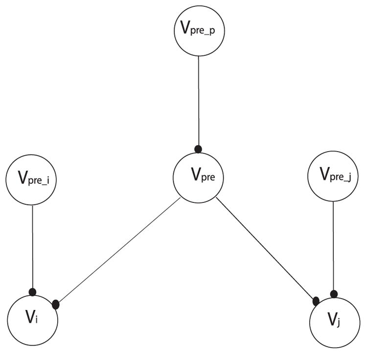
The network used in the proof of theorem 4.

From lemma 2, we have, for any neuron p ∈ {pre},

$$\text{Cov}[V_i,V_p]=-\left(\sum _{k\in \{{\mathit{pre}}_i\}}{g}_{k\to i}\text{Cov}[V_k,V_p]+\sum _{k\in \left\{\mathit{pre}\right\}}{g}_{k\to i}\text{Cov}[V_k,V_p]+\sum _{k\in \{{\mathit{pre}}_p\}}{g}_{k\to p}\text{Cov}[V_k,V_i]\right)/2g_l,$$ (A.32)

$$\begin{gathered} \text{Cov}[V_j,V_p] \\ =-\left(\sum _{k\in \{{\mathit{pre}}_j\}}{g}_{k\to j}\text{Cov}[V_k,V_p]+\sum _{k\in \left\{\mathit{pre}\right\}}{g}_{k\to j}\text{Cov}[V_k,V_p]+\sum _{k\in \{{\mathit{pre}}_p\}}{g}_{k\to p}\text{Cov}[V_k,V_j]\right)/2g_l. \end{gathered}$$ (A.33)

For simplicity, we define

$$\begin{gathered} \sum _{k\in \{{\mathit{pre}}_j\}}{g}_{k\to j}\text{Cov}[V_k,V_p]=C_p, \\ \sum _{k\in \{{\mathit{pre}}_i\}}{g}_{k\to i}\text{Cov}[V_k,V_p]=D_p, \\ \sum _{k\in \{{\mathit{pre}}_p\}}{g}_{k\to p}\text{Cov}[V_k,V_j]=E_p, \\ \sum _{k\in \{{\mathit{pre}}_p\}}{g}_{k\to p}\text{Cov}[V_k,V_i]=F_p. \end{gathered}$$ (A.34)

From lemma 2, we also have

$$\text{Cov}[V_i,V_j]=-\left(\sum _{k\in \{{\mathit{pre}}_i\}}{g}_{k\to i}\text{Cov}[V_k,V_j]+\sum _{k\in \{{\mathit{pre}}_j\}}{g}_{k\to j}\text{Cov}[V_k,V_i]+\sum _{k\in \left\{\mathit{pre}\right\}}{g}_{k\to i}\text{Cov}[V_k,V_j]+\sum _{k\in \left\{\mathit{pre}\right\}}{g}_{k\to j}\text{Cov}[V_k,V_i]\right)/2g_l.$$ (A.35)

For simplicity, we define

$$\begin{gathered} \sum _{k\in \{{\mathit{pre}}_i\}}{g}_{k\to i}\text{Cov}[V_k,V_j]=A, \\ \sum _{k\in \{{\mathit{pre}}_j\}}{g}_{k\to j}\text{Cov}[V_k,V_i]=B. \end{gathered}$$ (A.36)

Plug in equations A.32 and A.33 to A.35, and we have

$$\text{Cov}[V_i,V_j]=\sum _{p\in \left\{\mathit{pre}\right\}}\frac{g_{p\to i}}{4g_l^2}\left(\sum _{k\in \left\{\mathit{pre}\right\}}{g}_{k\to j}\text{Cov}[V_k,V_p]+C_p+E_p\right)+\sum _{p\in \left\{\mathit{pre}\right\}}\frac{g_{p\to j}}{4g_l^2}\left(\sum _{k\in \left\{\mathit{pre}\right\}}{g}_{k\to i}\text{Cov}[V_k,V_p]+D_p+F_p\right)-\frac{A}{2g_l}-\frac{B}{2g_l}.$$ (A.37)

Now we look at the differential covariance between neuron i and neuron j:

$$\text{Cov}[\frac{d{V}_i}{dt},V_j]=\sum _{k\in \{{\mathit{pre}}_i\}}{g}_{k\to i}\text{Cov}[V_k,V_j]+\sum _{k\in \left\{\mathit{pre}\right\}}{g}_{k\to i}\text{Cov}[V_k,V_j]+g_l\mathit{Cov}[V_i,V_j].$$ (A.38)

Plug in equations A.33 and A.37 and we have:

$$\begin{gathered} \text{Cov}\left[\frac{d{V}_i}{dt},V_j\right] \\ =A+\sum _{p\in \left\{\mathit{pre}\right\}}\frac{-g_{p\to i}}{2g_l}\left(\sum _{k\in \left\{\mathit{pre}\right\}}{g}_{k\to j}\text{Cov}[V_k,V_p]+C_p+E_p\right) \\ +g_l[\sum _{p\in \left\{\mathit{pre}\right\}}\frac{g_{p\to i}}{4g_l^2}\left(\sum _{k\in \left\{\mathit{pre}\right\}}{g}_{k\to j}\text{Cov}[V_k,V_p]+C_p+E_p\right) \\ +\sum _{p\in \left\{\mathit{pre}\right\}}\frac{g_{p\to j}}{4g_l^2}\left(\sum _{k\in \left\{\mathit{pre}\right\}}{g}_{k\to i}\text{Cov}[V_k,V_p]+D_p+F_p\right)-\frac{A}{2g_l}-\frac{B}{2g_l}] \\ =\frac{A}{2}-\frac{B}{2}+\sum _{p\in \left\{\mathit{pre}\right\}}\frac{g_{p\to j}}{4g_l}(D_p+F_p)-\sum _{p\in \left\{\mathit{pre}\right\}}\frac{g_{p\to i}}{4g_l}(C_p+E_p). \end{gathered}$$ (A.39)

Note:

• There is no physical connection between a neuron in {pre_i} and neuron j; otherwise, this neuron belongs to {pre}. Therefore, from theorem 2, A is $O(\frac{g_{\mathit{syn}}^2}{g_l^3})\ast g_{k\to i}=O(\frac{g_{\mathit{syn}}^3}{g_l^3})$.

• There is no physical connection between a neuron in {pre_j} and neuron i; otherwise, this neuron belongs to {pre}. Therefore, from theorem 2, B is $O(\frac{g_{\mathit{syn}}^2}{g_l^3})\ast g_{k\to j}=O(\frac{g_{\mathit{syn}}^3}{g_l^3})$.

• There could be physical connections between neurons in {pre_p} and {pre_j}, so C_p is $O(\frac{g_{\mathit{syn}}}{g_l^2})\ast g_{k\to j}=O(\frac{g_{\mathit{syn}}^2}{g_l^2})$.

• There could be physical connections between neurons in {pre_p} and {pre_i}, so D_p is $O(\frac{g_{\mathit{syn}}}{g_l^2})\ast g_{k\to i}=O(\frac{g_{\mathit{syn}}^2}{g_l^2})$.

• There could be physical connections between neurons in {pre_p} and neuron j, so E_p is $O(\frac{g_{\mathit{syn}}}{g_l^2})\ast g_{k\to p}=O(\frac{g_{\mathit{syn}}^2}{g_l^2})$.

• There could be physical connections between neurons in {pre_p} and neuron i, so F_p is $O(\frac{g_{\mathit{syn}}}{g_l^2})\ast g_{k\to p}=O(\frac{g_{\mathit{syn}}^2}{g_l^2})$.

Therefore,

$$\begin{gathered} \text{Cov}\left[\frac{d{V}_i}{dt},V_j\right]=O\left(\frac{g_{\mathit{syn}}^3}{g_l^3}\right)-O\left(\frac{g_{\mathit{syn}}^3}{g_l^3}\right)+\sum _{p\in \left\{\mathit{pre}\right\}}\sum _{k\in \left\{\mathit{pre}\right\}}\frac{g_{p\to j}}{4g_l}\left(O\left(\frac{g_{\mathit{syn}}^2}{g_l^2}\right)+O\left(\frac{g_{\mathit{syn}}^2}{g_l^2}\right)\right)-\sum _{p\in \left\{\mathit{pre}\right\}}\sum _{k\in \left\{\mathit{pre}\right\}}\frac{g_{p\to i}}{4g_l}\left(O\left(\frac{g_{\mathit{syn}}^2}{g_l^2}\right)+O\left(\frac{g_{\mathit{syn}}^2}{g_l^2}\right)\right) \\ =O\left(\frac{g_{\mathit{syn}}^3}{g_l^3}\right). \end{gathered}$$ (A.40)

From lemma 3, we know that $\text{Cov}[V_i,\frac{d{V}_j}{dt}]$ is also $O(\frac{g_{\mathit{syn}}^3}{g_l^3})$.

Theorem 5

Type 1 false connection’s strength is reduced in differential covariance.

Proof

From theorems 1 and 2, we know that in the correlation method, the strength of a nonphysical connection ( $O(\frac{g_{\mathit{syn}}}{g_l^2})$) is $\frac{g_{\mathit{syn}}}{g_l}$ times that of a physical connection ( $O(\frac{g_{\mathit{syn}}^2}{g_l^3})$).

From theorems 3 and 4, we know that in the differential covariance method, the strength of a nonphysical connection ( $O(\frac{g_{\mathit{syn}}}{g_l})$) is $\frac{g_{\mathit{syn}}^2}{g_l^2}$ times that of a physical connection ( $O(\frac{g_{\mathit{syn}}^3}{g_l^3})$).

Because g_syn ≪ g_l, the relative strength of the nonphysical connections is reduced in the differential covariance method.

A.3 Directionality Information in Differential Covariance

Theorem 6

If neuron i projects to neuron j with an excitatory connection, $\text{Cov}[\frac{d{V}_i}{dt},V_j]>0$ and $\text{Cov}[V_i,\frac{d{V}_j}{dt}]<0$.

Proof

Given the model above, similar to theorem 4, from lemma 2, we have, for any neuron p ∈ {pre}:

$$\text{Cov}[V_i,V_p]=-\left(\sum _{k\in \{{\mathit{pre}}_i\}}{g}_{k\to i}\text{Cov}[V_k,V_p]+\sum _{k\in \left\{\mathit{pre}\right\}}{g}_{k\to i}\text{Cov}[V_k,V_p]+\sum _{k\in \{{\mathit{pre}}_p\}}{g}_{k\to p}\text{Cov}[V_k,V_i]\right)/2g_l,$$ (A.41)

$$\text{Cov}[V_j,V_p]=-\left(\sum _{k\in \{{\mathit{pre}}_j\}}{g}_{k\to j}\text{Cov}[V_k,V_p]+\sum _{k\in \left\{\mathit{pre}\right\}}{g}_{k\to j}\text{Cov}[V_k,V_p]+\sum _{k\in \{{\mathit{pre}}_p\}}{g}_{k\to p}\text{Cov}[V_k,V_j]+g_{i\to j}\mathit{Cov}[V_i,V_p]\right)/2g_l.$$ (A.42)

For simplicity, we define

$$\begin{gathered} \sum _{k\in \{{\mathit{pre}}_j\}}{g}_{k\to j}\text{Cov}[V_k,V_p]=C_p, \\ \sum _{k\in \{{\mathit{pre}}_i\}}{g}_{k\to i}\text{Cov}[V_k,V_p]=D_p, \\ \sum _{k\in \{{\mathit{pre}}_p\}}{g}_{k\to p}\text{Cov}[V_k,V_j]=E_p, \\ \sum _{k\in \{{\mathit{pre}}_p\}}{g}_{k\to p}\text{Cov}[V_k,V_i]=F_p. \end{gathered}$$ (A.43)

From lemma 2, we also have

$$\text{Cov}[V_i,V_j]=-(\sum _{k\in \{{\mathit{pre}}_i\}}{g}_{k\to i}\text{Cov}[V_k,V_j]+g_{i\to j}\text{Cov}[V_i,V_i]+\sum _{k\in \{{\mathit{pre}}_j\}}{g}_{k\to j}\text{Cov}[V_k,V_i]+\sum _{k\in \left\{\mathit{pre}\right\}}{g}_{k\to i}\text{Cov}[V_k,V_j]+\sum _{k\in \left\{\mathit{pre}\right\}}{g}_{k\to j}\text{Cov}[V_k,V_i])/2g_l$$ (A.44)

For simplicity, we define

$$\begin{gathered} \sum _{k\in \{{\mathit{pre}}_i\}}{g}_{k\to i}\text{Cov}[V_k,V_j]=A, \\ \sum _{k\in \{{\mathit{pre}}_j\}}{g}_{k\to j}\text{Cov}[V_k,V_i]=B. \end{gathered}$$ (A.45)

Plug in A, B, C_p, D_p, E_p, and F_p:

$$\begin{gathered} \text{Cov}[V_i,V_j] \\ =\sum _{p\in \left\{\mathit{pre}\right\}}\frac{g_{p\to i}}{4g_l^2}\left(\sum _{k\in \left\{\mathit{pre}\right\}}{g}_{k\to j}\text{Cov}[V_k,V_p]+C_p+E_p+g_{i\to j}\text{Cov}[V_i,V_p]\right) \\ +\sum _{p\in \left\{\mathit{pre}\right\}}\frac{g_{p\to j}}{4g_l^2}\left(\sum _{k\in \left\{\mathit{pre}\right\}}{g}_{k\to i}\text{Cov}[V_k,V_p]+D_p+F_p\right) \\ -\frac{A}{2g_l}-\frac{B}{2g_l}-\frac{g_{i\to j}\text{Cov}[V_i,V_i]}{2g_l}. \end{gathered}$$ (A.46)

Now we look at the differential covariance between neuron i and neuron j:

$$\text{Cov}\left[\frac{d{V}_i}{dt},V_j\right]=\frac{A}{2}-\frac{B}{2}+\sum _{p\in \left\{\mathit{pre}\right\}}\frac{g_{p\to j}}{4g_l}(D_p+F_p)-\sum _{p\in \left\{\mathit{pre}\right\}}\frac{g_{p\to i}}{4g_l}(C_p+E_p++g_{i\to j}\text{Cov}[V_i,V_p])-\frac{g_{i\to j}\text{Cov}[V_i,V_i]}{2}.$$ (A.47)

Note that in theorem 4, we already proved the scale of A, B, C_p, D_p, E_p, F_p. Also:

• There are physical connections between neurons in {pre} and neuron i, so g_i­→jCov[V_i, V_p] is $O(\frac{g_{\mathit{syn}}}{g_l^2})\ast g_{k\to p}=O(\frac{g_{\mathit{syn}}^2}{g_l^2})$.

• From lemma 1, the autocovariance of neuron i is $O(\frac{1}{g_l})$. So g_i­→jCov[V_i, V_i] is $O(\frac{1}{g_l})\ast g_{i\to j}=O(\frac{g_{\mathit{syn}}}{g_l})$.

Therefore, g_i→jCov[V_i, V_i] is the dominant term in $\text{Cov}[\frac{d{V}_i}{dt},V_j]$. Since Cov[V_i, V_i] > 0, for excitatory connection g_i→j > 0, $\text{Cov}[\frac{d{V}_i}{dt},V_j]<0$.

From lemma 3,

$$\text{Cov}\left[V_i,\frac{d{V}_j}{dt}\right]=-\text{Cov}\left[\frac{d{V}_i}{dt},V_j\right].$$ (A.48)

Therefore, $\text{Cov}[V_i,\frac{d{V}_j}{dt}]>0$.

Corollary 1

If neuron i projects to neuron j with an inhibitory connection, $\mathit{Cov}[\frac{d{V}_i}{dt},V_j]>0$ and $\mathit{Cov}[V_i,\frac{d{V}_j}{dt}]<0$.

Proof

The proof is similar to theorem 6. Again, we know g_i→jCov[V_i, V_i] is the dominant term in $\text{Cov}[\frac{d{V}_i}{dt},V_j]$. Since Cov[V_i, V_i] > 0, for an inhibitory connection g_i→j < 0, $\text{Cov}[\frac{d{V}_i}{dt},V_j]>0$.

From lemma 3,

$$\text{Cov}\left[V_i,\frac{d{V}_j}{dt}\right]=-\text{Cov}\left[\frac{d{V}_i}{dt},V_j\right].$$ (A.49)

Therefore, $\text{Cov}[V_i,\frac{d{V}_j}{dt}]<0$.

Appendix B: Benchmarked Methods

We compared our methods to a few popular methods.

B.1 Covariance Method

The covariance matrix is defined as

$${\text{COV}}_{x,y}=\frac{1}{N}\sum _{i=1}^N(x_i-{\mu }_x)(y_i-{\mu }_y),$$ (B.1)

where x and y are two variables and μ_x and μ_y are their population mean.

B.2 Precision Matrix

The precision matrix is the inverse of the covariance matrix:

$$P={\text{COV}}^{-1},$$ (B.2)

It can be considered one kind of partial correlation. Here we briefly review this derivation because we use it to develop our new method. The derivation is based on and adapted from Cox and Wermuth (1996).

We begin by considering a pair of variables (x, y) and remove the correlation in them introduced from a control variable z.

First, we define the covariance matrix as

$${\text{COV}}_{\mathit{xyz}}=\left[\begin{array}{ccc}{\sigma }_{xx}& {\sigma }_{xy}& {\sigma }_{xz}\\ {\sigma }_{yx}& {\sigma }_{yy}& {\sigma }_{yz}\\ {\sigma }_{zx}& {\sigma }_{zy}& {\sigma }_{zz}\end{array}\right].$$ (B.3)

By solving the linear regression problem,

$$\begin{gathered} w_x=\underset{w}{argmin}E{(x-w\ast z)}^2, \\ {w}_y=\underset{w}{argmin}E{(y-w\ast z)}^2. \end{gathered}$$ (B.4)

we have

$$\begin{gathered} w_x={\sigma }_{xz}{\sigma }_{zz}^{-1}, \\ {w}_y={\sigma }_{yz}{\sigma }_{zz}^{-1}. \end{gathered}$$ (B.5)

Then we define the residual of x, y as

$$\begin{gathered} r_x=x-w_x\ast z, \\ {r}_y=y-w_y\ast z. \end{gathered}$$ (B.6)

Therefore, the covariance of r_x, r_y is

$${\text{COV}}_{r_x,r_y}={\sigma }_{xy}-{\sigma }_{xz}\ast {\sigma }_{zz}^{-1}\ast {\sigma }_{yz}.$$ (B.7)

If we define the precision matrix as

$$P_{\mathit{xyz}}=\left[\begin{array}{ccc}{p}_{xx}& p_{xy}& p_{xz}\\ p_{yx}& p_{yy}& p_{yz}\\ p_{zx}& p_{zy}& p_{zz}\end{array}\right],$$ (B.8)

using Cramer’s rule, we have

$$p_{xy}=\frac{-\left|\begin{array}{cc}{\sigma }_{xy}& {\sigma }_{xz}\\ {\sigma }_{zy}& {\sigma }_{zz}\end{array}\right|}{\mid {\text{COV}}_{\mathit{xyz}}\mid }.$$ (B.9)

Therefore,

$$p_{xy}=\frac{-{\sigma }_{zz}}{\mid {\text{COV}}_{\mathit{xyz}}\mid }({\sigma }_{\mathit{xyz}}-{\sigma }_{xz}\ast {\sigma }_{zz}^{-1}\ast {\sigma }_{yz}).$$ (B.10)

So p_xy and COV_rx,ry differ by a ratio of $\frac{-{\sigma }_{zz}}{\mid {\mathit{COV}}_{\mathit{xyz}}\mid }$.

B.3 Sparse Latent Regularization

Prior studies (Banerjee, Ghaoui, d’Aspremont, & Natsoulis, 2006; Friedman, Hastie, & Tibshirani, 2008) have shown that regularizations can provide better a estimation if the ground-truth connection matrix has a known structure (e.g., sparse). For all data tested in this letter, the sparse latent regularization (Yatsenko et al., 2015) worked best. For a fair comparison, we applied the sparse latent regularization to both the precision matrix method and our differential covariance method.

In the original sparse latent regularization method, people made the assumption that a larger precision matrix S is the joint distribution of the p observed neurons and d latent neurons (Yatsenko et al., 2015):

$$S=\left(\begin{array}{cc}{S}_{11}& S_{12}\\ S_{21}& S_{22}\end{array}\right),$$

where S₁₁ corresponds to the observable neurons. If we can measure only the observable neurons, the partial correlation computed from the observed neural signals is

$$C_{ob}^{-1}=S_{ob}=S_{11}-S_{12}·S_{22}^{-1}·S_{21}$$ (B.11)

because the invisible latent neurons as shown in equation 2.2 introduce correlations into the measurable system. We denote this correlation introduced from the latent inputs as

$$L=S_{12}·S_{22}^{-1}·S_{21}.$$ (B.12)

If we can make the assumption that the connections between the visible neurons are sparse (S₁₁ is sparse and the number of latent neurons is much smaller than the number of visible neurons, that is, d ≪ p), then prior work (Chandrasekaran et al., 2011) has shown that if S_ob is known, S₁₁ is sparse enough and L’s rank is low enough (within the bound defined in Chandrasekaran et al., 2011); then the solution of

$$S_{11}-L=S_{ob}$$ (B.13)

is uniquely defined and can be solved by the following convex optimization problem,

$$\underset{S_{11},L}{argmin}{\left|\right|S_{11}\left|\right|}_1+\alpha \ast tr(L),$$ (B.14)

under the constraint that

$$S_{ob}=S_{11}-L$$ (B.15)

Here, || ||₁ is the L1-norm of a matrix, and tr() is the trace of a matrix. α is the penalty ratio between the L1-norm of S₁₁ and the trace of L and is set to $1/\sqrt{N}$ for all our estimations.

However, this method is used to regularize precision matrix. For our differential covariance estimation, we need to make small changes to the derivation. Note that if we assume that the neural signals of the latent neurons are known and let l be the indexes of these latent neurons, from section 2.2.2,

$${\mathrm{\Delta }}_{S_{i,j}}={\mathrm{\Delta }}_{P_{i,j}}-{\text{COV}}_{j,l}·{\text{COV}}_{l,l}^{-1}·{\mathrm{\Delta }}_{C_{i,l}}^T$$ (B.16)

removes the V_latent terms in equation 2.2.

Even if l is unknown,

$${\text{COV}}_{j,l}·{\text{COV}}_{l,l}^{-1}·{\mathrm{\Delta }}_{C_{i,l}}^T$$

is low rank because it is bounded by the dimensionality of COV_l,l, which is d. And Δ_S is the internal connection between the visible neurons, which should be a sparse matrix. Therefore, letting

$$\begin{gathered} S_{ob}={\mathrm{\Delta }}_P, \\ {S}_{11}={\mathrm{\Delta }}_S, \\ L=-{\mathit{COV}}_{j,l}·{\mathit{COV}}_{l,l}^{-1}·{\mathrm{\Delta }}_{C_{i,l}}^T, \end{gathered}$$ (B.17)

we can use the original sparse+latent method to solve for Δ_S. In this article, we used the inexact robust PCA algorithm (http://perception.csl.illinois.edu/matrix-rank/sample_code.html) to solve this problem (Lin, Liu, & Su, 2011).

B.4 The Generalized Linear Model Method

As summarized by Roudi et al. (2015), GLMs assume that every neuron spikes at a time-varying rate that depends on earlier spikes (both those of other neurons and its own) and on external covariates (such as a stimulus or other quantities measured in the experiment). As they explained, the influence of earlier spikes on the firing probability at a given time is assumed to depend on the time since they occurred. For each prepostsynaptic pair i, j, it is described by a function J_{i j} (τ) of this time lag (Roudi et al., 2015). In this article, we average this temporal dependent function J_{i j} (τ) over time to obtain the functional connectivity estimation of this method.

The spike trains used for the GLM method were computed using the spike detection algorithm from Quiroga, Nadasdy, and Ben-Shaul (2004) (https://github.com/csn-le/wave_clus). The article’s default parameter set is used except that the maximum detection threshold is increased. The code is provided in our github repository (https://github.com/tigerwlin/diffCov/blob/master/spDetect.m) for reference. The GLM code was obtained from Pillow et al. (2008) (http://pillowlab.princeton.edu/code_GLM.html) and applied on the spike trains.

Appendix C: Details about the Thalamocortical Model

C.1 Intrinsic Currents

For the thalamocortical model, a conductance-based formulation was used for all neurons. The cortical neuron consisted of two compartments, dendritic and axo-somatic compartments, similar to previous studies (Bazhenov et al., 2002; Chen et al., 2012; Bonjean et al., 2011) and is described by the following equations,

$$\begin{gathered} C_m\frac{d{V}_D}{dt}=-I_d^{K-\mathit{leak}}-I_d^{\mathit{leak}}-I_d^{Na}-I_d^{\mathit{Nap}}-I_d^{Ca}-I_d^{Km}-I^{\mathit{syn}}, \\ {g}_c^s(V_S-V_D)=-I_S^{Na}-I_S^K-I_S^{\mathit{Nap}}, \end{gathered}$$ (C.1)

where the subscripts s and d correspond to axo-somatic and dendritic compartment, I^leak is the Cl⁻ leak currents, I^Na is fast Na⁺ channels, I^Nap is persistent sodium current, I^K is fast delayed rectifier K⁺ current, I^Km is slow voltage-dependent noninactivating K⁺ current, I^KCa is slow Ca²⁺-dependent K⁺ current, I^Ca is high-threshold Ca²⁺ current, I^h is hyperpolarization-activated depolarizing current, and I^syn is the sum of synaptic currents to the neuron. All intrinsic currents were of the form g(V − E), where g is the conductance, V is the voltage of the corresponding compartment, and E is the reversal potential. The detailed descriptions of individual currents are provided in previous publications (Bazhenov et al., 2002; Chen et al., 2012). The conductances of the leak currents were 0.007 mS/cm² for $I_d^{K-\mathit{leak}}$ and 0.023 mS/cm² for $I_d^{\mathit{leak}}$. The maximal conductances for different currents were ${\mathrm{I}}_d^{\mathit{Nap}}:2.0\text{mS}/{\text{cm}}^2;{\mathrm{I}}_d^{Na}:0.8\text{mS}/{\text{cm}}^2;{\mathrm{I}}_d^{Km}:0.012\text{mS}/{\text{cm}}^2;{\mathrm{I}}_d^{\mathit{KCa}}:0.015\text{mS}/{\text{cm}}^2;{\mathrm{I}}_d^{Km}:0.012\text{mS}/{\text{cm}}^2;{\mathrm{I}}_s^{Na}:3000\text{mS}/{\text{cm}}^2;{\mathrm{I}}_s^K:200\text{mS}/{\text{cm}}^2$; and ${\mathrm{I}}_s^{\mathit{Nap}}:15\text{mS}/{\text{cm}}^2$. C_m was 0.075μF/cm².

The following describes the IN neurons:

$$\begin{gathered} C_m\frac{d{V}_D}{dt}=-I_d^{K-\mathit{leak}}-I_d^{\mathit{leak}}-I_d^{Na}-I_d^{Ca}-I_d^{\mathit{KCa}}-I_d^{Km}-I^{\mathit{syn}} \\ {g}_c^s(V_S-V_D)=-I_S^{Na}-I_S^K. \end{gathered}$$ (C.2)

The conductances for leak currents for IN neurons were 0.034 mS/cm² for ${\mathrm{I}}_d^{K-\mathit{leak}}$ and 0.006 mS/cm² for ${\mathrm{I}}_d^{\mathit{leak}}$. Maximal conductances for other currents were ${\mathrm{I}}_d^{Na}:0.8\text{mS}/{\text{cm}}^2;{\mathrm{I}}_d^{Ca}:0.012\text{mS}/{\text{cm}}^2;{\mathrm{I}}_d^{\mathit{KCa}}:0.015\text{mS}/{\text{cm}}^2;{\mathrm{I}}_d^{Km}:0.012\text{mS}/{\text{cm}}^2{;\mathrm{I}}_s^{Na}:2500\text{mS}/{\text{cm}}^2$ and ${\mathrm{I}}_s^K:200\text{mS}/{\text{cm}}^2$.

The TC neurons consisted of only single compartment and are described as follows:

$$\frac{d{V}_D}{dt}=-I^{K-\mathit{leak}}-I^{\mathit{leak}}-I^{Na}-I^K-I^{\mathit{LCa}}-I^h-I^{\mathit{syn}}.$$ (C.3)

The conductances of leak currents were I^leak: 0.01 mS/cm²; I^K−leak: 0.007 mS/cm²; The maximal conductances for other currents were: fast Na⁺ (I^Na) current: 90 mS/cm²; fast K⁺ (I^k) current: 10 mS/cm²; low-threshold Ca²⁺(I^LCa) current: 2.5 mS/cm²; and hyperpolarization-activated depolarizing current (I^h): 0.015 mS/cm².

The RE cells were also modeled as a single compartment neuron:

$$\frac{d{V}_D}{dt}=-I^{K-\mathit{leak}}-I^{\mathit{leak}}-I^{Na}-I^K-I^{\mathit{LCa}}-I^h-I^{\mathit{syn}}.$$ (C.4)

The conductances for leak currents were I^leak: 0.05 mS/cm² and I^K−leak: 0.016 mS/cm². The maximal conductances for other currents were fast Na⁺ (I^Na) current: 100 mS/cm²; fast K⁺ (I^K) current: 10 mS/cm²; and low-threshold Ca²⁺(I^LCa) current: 2.2 mS/cm².

C.2 Synaptic Currents

GABA-A, NMDA and AMPA synaptic currents were described by first-order activation schemes (Timofeev, Grenier, Bazhenov, Sejnowski, & Steriade, 2000). The equations for all synaptic currents used in this model are given in our previous publications (Bazhenov et al., 2002; Chen et al., 2012). We mention only the relevant equations:

$$\begin{gathered} I_{\mathit{syn}}^{\mathit{AMPA}}=g_{\mathit{syn}}[O](V-E_{\mathit{AMPA}}), \\ {I}_{\mathit{syn}}^{\mathit{NMDA}}=g_{\mathit{syn}}[O](V-E_{\mathit{NMDA}}), \\ {I}_{\mathit{syn}}^{\mathit{GABA}}=g_{\mathit{syn}}[O](V-E_{\mathit{GABA}}). \end{gathered}$$ (C.5)

References

- Banerjee O, Ghaoui LE, d’Aspremont A, Natsoulis G. Convex optimization techniques for fitting sparse gaussian graphical models. Proceedings of the 23rd International Conference on Machine Learning; New York: ACM; 2006. pp. 89–96. [Google Scholar]
- Battistin C, Hertz J, Tyrcha J, Roudi Y. Belief propagation and replicas for inference and learning in a kinetic Ising model with hidden spins. Journal of Statistical Mechanics: Theory and Experiment. 2015;2015(5):P05021. [Google Scholar]
- Bazhenov M, Timofeev I, Steriade M, Sejnowski TJ. Model of thalamocortical slow-wave sleep oscillations and transitions to activated states. Journal of Neuroscience. 2002;22(19):8691–8704. doi: 10.1523/JNEUROSCI.22-19-08691.2002. [DOI] [PMC free article] [PubMed] [Google Scholar]
- Bonjean M, Baker T, Lemieux M, Timofeev I, Sejnowski T, Bazhenov M. Corticothalamic feedback controls sleep spindle duration in vivo. Journal of Neuroscience. 2011;31(25):9124–9134. doi: 10.1523/JNEUROSCI.0077-11.2011. [DOI] [PMC free article] [PubMed] [Google Scholar]
- Burkitt AN. A review of the integrate-and-fire neuron model: I. Homogeneous synaptic input. Biological Cybernetics. 2006;95(1):1–19. doi: 10.1007/s00422-006-0068-6. [DOI] [PubMed] [Google Scholar]
- Capone C, Filosa C, Gigante G, Ricci-Tersenghi F, Del Giudice P. Inferring synaptic structure in presence of neural interaction time scales. PloS One. 2015;10(3):e0118412. doi: 10.1371/journal.pone.0118412. [DOI] [PMC free article] [PubMed] [Google Scholar]
- Chandrasekaran V, Sanghavi S, Parrilo PA, Willsky AS. Rank-sparsity incoherence for matrix decomposition. SIAM Journal on Optimization. 2011;21(2):572–596. [Google Scholar]
- Chen JY, Chauvette S, Skorheim S, Timofeev I, Bazhenov M. Interneuron-mediated inhibition synchronizes neuronal activity during slow oscillation. Journal of Physiology. 2012;590(16):3987–4010. doi: 10.1113/jphysiol.2012.227462. [DOI] [PMC free article] [PubMed] [Google Scholar]
- Cox DR, Wermuth N. Multivariate dependencies: Models, analysis and interpretation. Boca Raton, FL: CRC Press; 1996. [Google Scholar]
- Destexhe A. Spike-and-wave oscillations based on the properties of GABAB receptors. Journal of Neuroscience. 1998;18(21):9099–9111. doi: 10.1523/JNEUROSCI.18-21-09099.1998. [DOI] [PMC free article] [PubMed] [Google Scholar]
- Dunn B, Roudi Y. Learning and inference in a nonequilibrium Ising model with hidden nodes. Physical Review E. 2013;87(2):022127. doi: 10.1103/PhysRevE.87.022127. [DOI] [PubMed] [Google Scholar]
- Fan H, Shan X, Yuan J, Ren Y. Covariances of linear stochastic differential equations for analyzing computer networks. Tsinghua Science and Technology. 2011;16(3):264–271. [Google Scholar]
- Friedman J, Hastie T, Tibshirani R. Sparse inverse covariance estimation with the graphical lasso. Biostatistics. 2008;9(3):432–441. doi: 10.1093/biostatistics/kxm045. [DOI] [PMC free article] [PubMed] [Google Scholar]
- Friston KJ. Functional and effective connectivity: Areview. Brain Connectivity. 2011;1(1):13–36. doi: 10.1089/brain.2011.0008. [DOI] [PubMed] [Google Scholar]
- Harrison L, Penny WD, Friston K. Multivariate autoregressive modeling of FMRI time series. NeuroImage. 2003;19(4):1477–1491. doi: 10.1016/s1053-8119(03)00160-5. [DOI] [PubMed] [Google Scholar]
- Huang H. Sparse Hopfield network reconstruction with 1 regularization. European Physical Journal B. 2013;86(11):1–7. [Google Scholar]
- Kandel ER, Markram H, Matthews PM, Yuste R, Koch C. Neuroscience thinks big (and collaboratively) Nature Reviews Neuroscience. 2013;14(9):659–664. doi: 10.1038/nrn3578. [DOI] [PubMed] [Google Scholar]
- Lánskỳ P, Rospars JP. Ornstein-Uhlenbeck model neuron revisited. Biological Cybernetics. 1995;72(5):397–406. [Google Scholar]
- Lin Z, Liu R, Su Z. Linearized alternating direction method with adaptive penalty for low-rank representation. In: Shawe-Taylor J, Zemel RS, Bartlett PL, Pereira F, Weinberger KQ, editors. Advances in neural information processing systems. Vol. 24. Red Hook, NY: Curran; 2011. pp. 612–620. [Google Scholar]
- McIntosh A, Gonzalez-Lima F. Structural modeling of functional neural pathways mapped with 2-deoxyglucose: Effects of acoustic startle habituation on the auditory system. Brain Research. 1991;547(2):295–302. doi: 10.1016/0006-8993(91)90974-z. [DOI] [PubMed] [Google Scholar]
- Nunez P, Srinivasan R. Electric fields of the brain. New York: Oxford University Press; 2005. [Google Scholar]
- Okatan M, Wilson MA, Brown EN. Analyzing functional connectivity using a network likelihood model of ensemble neural spiking activity. Neural Computation. 2005;17(9):1927–1961. doi: 10.1162/0899766054322973. [DOI] [PubMed] [Google Scholar]
- Pernice V, Rotter S. Reconstruction of sparse connectivity in neural networks from spike train covariances. Journal of Statistical Mechanics: Theory and Experiment. 2013;2013(3):P03008. [Google Scholar]
- Pillow JW, Shlens J, Paninski L, Sher A, Litke AM, Chichilnisky E, Simoncelli EP. Spatio-temporal correlations and visual signalling in a complete neuronal population. Nature. 2008;454(7207):995–999. doi: 10.1038/nature07140. [DOI] [PMC free article] [PubMed] [Google Scholar]
- Quan T, Liu X, Lv X, Chen WR, Zeng S. Method to reconstruct neuronal action potential train from two-photon calcium imaging. Journal of Biomedical Optics. 2010;15(6):066002. doi: 10.1117/1.3505021. [DOI] [PMC free article] [PubMed] [Google Scholar]
- Quiroga RQ, Nadasdy Z, Ben-Shaul Y. Unsupervised spike detection and sorting with wavelets and superparamagnetic clustering. Neural Computation. 2004;16(8):1661–1687. doi: 10.1162/089976604774201631. [DOI] [PubMed] [Google Scholar]
- Rahmati V, Kirmse K, Marković D, Holthoff K, Kiebel SJ. Inferring neuronal dynamics from calcium imaging data using biophysical models and Bayesian inference. PLoS Comput Biol. 2016;12(2):e1004736. doi: 10.1371/journal.pcbi.1004736. [DOI] [PMC free article] [PubMed] [Google Scholar]
- Ricciardi LM, Sacerdote L. The Ornstein-Uhlenbeck process as a model for neuronal activity. Biological Cybernetics. 1979;35(1):1–9. doi: 10.1007/BF01845839. [DOI] [PubMed] [Google Scholar]
- Roudi Y, Dunn B, Hertz J. Multi-neuronal activity and functional connectivity in cell assemblies. Current Opinion in Neurobiology. 2015;32:38–44. doi: 10.1016/j.conb.2014.10.011. [DOI] [PubMed] [Google Scholar]
- Roudi Y, Hertz J. Mean field theory for nonequilibrium network reconstruction. Physical Review Letters. 2011;106(4):048702. doi: 10.1103/PhysRevLett.106.048702. [DOI] [PubMed] [Google Scholar]
- Schneidman E, Berry MJ, Segev R, Bialek W. Weak pairwise correlations imply strongly correlated network states in a neural population. Nature. 2006;440(7087):1007–1012. doi: 10.1038/nature04701. [DOI] [PMC free article] [PubMed] [Google Scholar]
- Stetter O, Battaglia D, Soriano J, Geisel T. Model-free reconstruction of excitatory neuronal connectivity from calcium imaging signals. PLoS Comput Biol. 2012;8(8):e1002653. doi: 10.1371/journal.pcbi.1002653. [DOI] [PMC free article] [PubMed] [Google Scholar]
- Stevenson IH, Kording KP. How advances in neural recording affect data analysis. Nature Neuroscience. 2011;14(2):139–142. doi: 10.1038/nn.2731. [DOI] [PMC free article] [PubMed] [Google Scholar]
- Stevenson IH, Rebesco JM, Miller LE, Körding KP. Inferring functional connections between neurons. Current Opinion in Neurobiology. 2008;18(6):582–588. doi: 10.1016/j.conb.2008.11.005. [DOI] [PMC free article] [PubMed] [Google Scholar]
- Timofeev I, Grenier F, Bazhenov M, Sejnowski T, Steriade M. Origin of slow cortical oscillations in deafferented cortical slabs. Cerebral Cortex. 2000;10(12):1185–1199. doi: 10.1093/cercor/10.12.1185. [DOI] [PubMed] [Google Scholar]
- Truccolo W, Eden UT, Fellows MR, Donoghue JP, Brown EN. A point process framework for relating neural spiking activity to spiking history, neural ensemble, and extrinsic covariate effects. Journal of Neurophysiology. 2005;93(2):1074–1089. doi: 10.1152/jn.00697.2004. [DOI] [PubMed] [Google Scholar]
- Uhlenbeck GE, Ornstein LS. On the theory of the Brownian motion. Physical Review. 1930;36(5):823. [Google Scholar]
- Vogelstein JT, Watson BO, Packer AM, Yuste R, Jedynak B, Paninski L. Spike inference from calcium imaging using sequential Monte Carlo methods. Biophysical Journal. 2009;97(2):636–655. doi: 10.1016/j.bpj.2008.08.005. [DOI] [PMC free article] [PubMed] [Google Scholar]
- Winterhalder M, Schelter B, Hesse W, Schwab K, Leistritz L, Klan D, … Witte H. Comparison of linear signal processing techniques to infer directed interactions in multivariate neural systems. Signal Processing. 2005;85(11):2137–2160. [Google Scholar]
- Yatsenko D, Josić K, Ecker AS, Froudarakis E, Cotton RJ, Tolias AS. Improved estimation and interpretation of correlations in neural circuits. PLoS Computational Biology. 2015;2:199–207. doi: 10.1371/journal.pcbi.1004083. [DOI] [PMC free article] [PubMed] [Google Scholar]
Associated Data
This section collects any data citations, data availability statements, or supplementary materials included in this article.