Stable, Robust Hybrid Zero Dynamics Control of Powered Lower-Limb Prostheses

Abstract

To improve the quality of life for lower-limb amputees, powered prostheses are being developed. Advanced control schemes from the field of bipedal robots, such as hybrid zero dynamics (HZD), may provide great performance. HZD-based control specifies the motion of the actuated joints using output functions to be zeroed, and the required torques are calculated using input-output linearization. For one-step periodic gaits, there is an analytic metric of stability. To apply HZD-based control on a powered prosthesis, several modifications must be made. Because the prosthesis and amputee are only connected via the socket, the prosthesis controller does not have access to the full state of the biped, which decentralizes the form of the input-output linearization. The differences between the amputated and contralateral sides result in a two-step periodic gait, which requires the orbital stability metric to be extended. In addition, because human gait is variable, the prosthesis controller must be robust to continuous moderate perturbations. This robustness is proved using local input-to-state stability and demonstrated with simulations of an above-knee amputee model.

I.Introduction

Of the approximately 623,000 people living with major lower-limb loss in the United States [1], the majority use a prosthesis daily [2]. Unfortunately, current commercially available prostheses do not completely restore the lost function of the joints. Amputee gait tends to be slower [3], less efficient [4], and less robust [5] than healthy gait. In addition, amputees typically exhibit significant asymmetry between sides [6], which may increase the risk for secondary conditions [7].

Even though human joints generate significant positive work to contribute to gait energetics during gait [8], most prostheses cannot. To improve amputee gait quality, several groups have developed powered prostheses capable of generating positive work for both above- [9], [10] and below-knee amputees [11], [12]. The controllers typically divide the stride into multiple periods with a distinct control law for each period [13], resulting in large numbers of parameters to be (manually) tuned [14]. One of the more common control methods is impedance-based control, which effectively defines a spring and damper system for each gait period [9], [15]. For basic impedance-based control, the stride is divided into four or five sequential periods and the controller progresses to the next period when the kinematic or kinetic switching criteria has been met [9]. Because the impedance parameters are constant within a period, the prosthesis passively guarantees a stable equilibrium configuration if the parameters are properly chosen but cannot accommodate period-shifting disturbances or react in a manner that requires positive work. Rather, it is left to the amputee to react to perturbations and actively stabilize the entire gait cycle.

A control strategy that actively reacts to perturbations might relieve the amputee of some of the cognitive and physical effort of gait. To accomplish this, the controller must be able to vary joint positions and/or torques in a continuous manner so that it can react to perturbations, rather than using a few set points as in impedance-based control. This requires the progression of the gait cycle to be parameterized in a unified, continuous manner. Recent work has shown that human joint patterns are parameterized well by a phase variable [16], [17], which is a kinematic quantity that measures how far a step (or stride) has progressed. In addition, pre-clinical work has demonstrated that phase-based controllers can successfully control powered prostheses [18], [19], although determination of the best control strategy is still very much an open question.

A promising phase-based control framework is hybrid zero dynamics (HZD). HZD-based control has successfully generated stable walking for 2D-point- [20], 3D-point- [21], and 2D-curved-foot [22] bipedal robots. In addition, HZD-based models can predict healthy human walking [23] and robustly enforce simplified model dynamics [24]. Under an HZD-based control paradigm, bipeds are assumed to be underactuated, the step is driven by the phase variable, and each step is divided into a finite-time single support period and an instantaneous, impulsive double-support period [20]. During the single support period, the motion of the actuated degrees of freedom (DoF) are typically encoded in output functions to be zeroed [25] although other options are possible [26]. The joint torques are determined using input-output linearization. The motion of the unactuated DoF are captured in the zero dynamics. Since gait is typically assumed to be one-step periodic, orbital stability can be evaluated using the method of Poincaré [20]. If the desired gait respects the impact dynamics (i.e. is hybrid invariant), then orbital stability can be evaluated using just the lower-dimensional zero dynamics [27], [28].

HZD-based control becomes more challenging on a practical prosthesis, which only has information about its own state (from onboard sensors) and not the full biped state as in robotics. Thus, existing formulations for HZD-based control cannot be directly applied to prosthesis control. A related problem arises in multi-machine power systems. Similar to the human-prosthesis system, the dynamics of each subsystem are both nonlinear and coupled [29]. For a prosthesis, the challenge lies in deriving the input-output linearizing controller for a coupled periodic mechanical system, rather than an aperiodic electrical system. Because the prosthesis is attached to the human via a socket, the human and prosthesis interact through the socket interaction force. This coupling force represents the effects of one subsystem on the other and can be used to account for the human's dynamics in the prosthesis controller. One control approach is to account for the forces during gait design and then ignore them in the controller, but this neglects the human input to the prosthesis [30]. The approach taken here is to directly account for the socket interaction force. In hardware, the socket interaction force can be measured, but equations to calculate it in simulation must be derived.

An additional challenge in controlling a prosthesis is the variability in human gait [31]. Because robot gaits are typically designed to be periodic, most formal stability metrics assume periodicity. There are some metrics that measure robustness to larger perturbations and aperiodic gait [32]–[36], but most are either difficult to apply or inappropriate for human gait. Perhaps the most promising robustness metric is input-to-state stability (ISS) [36] which can be used to prove bounded output for bounded variability. Alternatively, robustness can be assessed by simulating a large number of aperiodic steps and seeing if and when the biped falls [35]. This requires that the simulated human variability be realistic, and that the human model be somewhat predictive of human behavior when interacting with the prosthesis.

Despite these challenges, pre-clinical work has shown that a powered above-knee prosthesis controlled with an HZD-like controller during stance and an impedance-based controller during swing allows amputees to walk at a variety of speeds and ground slopes [19]. That work did not generalize the input-output linearizing controller to the prosthesis swing phase or, to allow for more realistic modeling, to the human subsystem. The work also did not make use of the reduced order system to develop an analytical metric of stability, in part because the output functions were not hybrid invariant.

The present work extends the modeling and control methods needed to formally develop hybrid invariant, input-output linearizing prosthesis controllers for the entire stride and to predictively test these controllers in simulation. Specifically, using an asymmetric biped, this work

• constructs input-output linearizing controllers for the entire gait cycle for both the human and prosthesis using only information available to each subsystem,

• derives conditions to ensure hybrid invariance,

• develops an analytic metric of stability for asymmetric gait using a reduced order system, and

• proves and demonstrates that the amputee-prosthesis system is robust to human-like kinematic variation.

Some of the results (namely, the controller and stability metric) were preliminarily presented in [37]. The present paper provides a comprehensive discussion of the full theoretical framework needed to formally derive hybrid invariant, input-output linearizing controllers for a biped with two connected but distinct subsystems. It also presents realistic simulation results demonstrating both orbital stability and robustness to human-like variability. While the presented simulation results are for an above-knee amputee, the theoretical results are equally applicable to a below-knee amputee.

II. Model

A. Physical Model

The full planar model of the unilateral above-knee amputee consists of seven leg segments plus a point mass at the hip to represent the upper body (Fig. 1, [37]). Rather than model all of the DoF of the foot, the function of the foot and ankle is modeled using a circular foot plus an ankle joint [23] to capture both the center of pressure movement [38] and the positive work performed at the stance ankle [39]. To account for the lack of information transmitted between the human and prosthesis, the full model can be divided into a prosthesis subsystem and a human subsystem [19]. The prosthesis subsystem consists of the prosthetic thigh, shank, and foot. The human subsystem consists of the contralateral (non-amputated side) thigh, shank, and foot, the residual thigh on the amputated side, and the point mass at the hip. To ensure the modeling equations are accurate, the following hypotheses must hold:

Fig. 1.

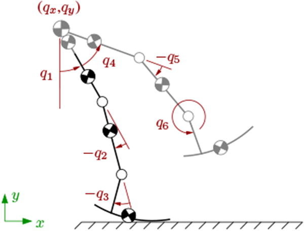
Schematic of the above-knee amputee model, with the prosthesis shown in black and the human shown in gray. The generalized coordinates are shown in red. Both legs have actuated knee and ankle joints. In addition, there is one actuated rotational DoF at the hip. The foot-ground interface is unactuated. The prosthesis generalized coordinates are the hip position (q_x and q_y), the unactuated absolute angle (q₁), and the actuated prosthesis joint angles (q₂ and q₃). The human generalized coordinates are the hip position (q_x and q_y), the unactuated absolute angle (q₁), and the actuated human joint angles (q₄, q₅, and q₆).

Hypothesis 1

1. The prosthetic thigh and residual thigh (i.e., stump) are rigidly attached.

2. Both the prosthetic thigh and the stump have non-zero length.

3. The biped rolls without slip. Thus, the foot-ground connection is unactuated and has no applied torque.

4. All remaining joints are actuated using torque generators with no dynamics of their own. Thus, the biped is underactuated by one DoF.

5. The vertical ground reaction force (GRF) at the stance foot is positive. The swing foot has no GRF.

To describe the motion of the biped, each subsystem has its own set of generalized coordinates. In general, each subsystem's generalized coordinates should be the relative angles of its actuated joints, the absolute angle of the unactuated DoF, and the Cartesian coordinates of a fixed point on the biped. For this model (Fig. 1), q₁is the absolute angle, and the fixed point is the hip position (q_x, q_y). The actuated joint angles are q₂-q₆. Thus, the generalized coordinates are q_P= [q₁ q₂ q₃ q_x q_y]^T for the prosthesis and q_H = [q₁ q₄ q₅ q₆ q_x q_y]^T for the human. Each subsystem also has its own joint torques: u_P=[u₂ u₃]^T for the prosthesis and u_H =[u₄ u₅ u₆]^T for the human. Because the prosthesis is rigidly attached to the residual limb, forces and moments are transmitted through this interface and provide an indirect measure of the motion of both subsystems via the socket interaction force F = [F_x F_y F_M]^T. The vector F contains two forces (F_x, F_y) and a moment (F_M), but will be referred to as the socket interaction force for conciseness. The leg in stance also experiences horizontal and vertical GRF G = [G_x G_y]^T.

Remark. Hypothesis 1.2 is needed to ensure that the joint torques u and socket interaction torque F_M are unique. If the connection between the prosthetic thigh and stump is at a joint, there is no mathematical distinction between the actuator torque and the socket interaction torque.

Each stride progresses through a prosthesis stance period, an instantaneous impact, a contralateral stance period, and a second instantaneous impact (Fig. 2). The two stance periods are modeled with continuous, second-order differential equations. The two impact periods are modeled using an algebraic mapping relating the state just before impact to the state just after impact. The stance leg switches during the impact period.

Fig. 2.

The periodic gait. The ξ terms are the zero dynamics coordinates used for the reduced system (Sec. IV). For simulation, a stride starts just after the transition from contralateral stance to prosthesis stance and proceeds through the prosthesis stance period, an impact event, the contralateral stance period and a second impact.

B. Single Support Periods

During the single support periods, the motion of each subsystem can be described using that subsystem's generalized coordinates and the forces acting on that subsystem [37]. The equations of motion (EoM) relating the generalized coordinates to the forces are:

$$M_i{\ddot{q}}_i+C_i{\dot{q}}_i+N_i-E_{ij}^{T}G=B_i{u}_i+J_i^{T}F.$$ (1)

Throughout this paper, the subscript i indicates which subsystem the term is for, with P indicating the prosthesis subsystem and H indicating the human subsystem. The subscript j indicates which leg is in stance, with P indicating the prosthesis and C indicating the contralateral leg. M_i(q_i) is the 𝒩_i × 𝒩_i inertia matrix, C_i(q_i,q̇_i) is the 𝒩_i × 𝒩_i matrix containing the centripetal and Coriolis terms, N_i(q_i) is the 𝒩_i × 1 gravity vector, E_ij(q_i) is a 2 × 𝒩_i constraint matrix, B_i is the 𝒩_i × ℳ_i matrix relating the input torques to the generalized coordinates, and J_i(q_i) is the 3 × 𝒩_i matrix relating the socket interaction forces to the generalized coordinates. For an above-knee amputee, there are 𝒩_P =5 generalized prosthesis coordinates, ℳ_P = 2 prosthesis joint torques, 𝒩_H = 6 human generalized coordinates, and ℳ_H = 3 human joint torques. The matrices are found using the method of Lagrange. Except for the constraint matrix E_ij(q_i), all matrices are identical regardless of which leg is in stance. To attach the biped to the ground, the constraint equation is used¹ [40]:

$$E_{ij}(q_i){\dot{q}}_i=0.$$ (2)

Lemma 1. Each row in E_ij(q_i) is independent.

Proof. Without loss of generality, assume the last two entries in q_i are the orthogonal Cartesian coordinates q_x and q_y oriented so that q_x is aligned with the direction of travel. Because the stance foot cannot penetrate the ground (Hypothesis 1.5), there is a constraint in the vertical (or q_y) direction. Because the stance foot rolls without slip (Hypothesis 1.3), there is also a constraint in the horizontal (or q_x) direction. These constraints can be written in vector form using standard kinematic methods as

$$0={\upsilon }_F+{\upsilon }_{\text{rel}}(q_i,{\dot{q}}_i)$$ (3)

where ν_F=[q̇_x q̇_y ]^T is the velocity of the fixed point on the biped and ν_rel is the velocity of the foot relative to the velocity of the fixed point [22]. The relative velocity does not depend on q̇_x or q̇_y. Eq. 3 is multiplied by dt to obtain the virtual displacements and rearranged into the form 0 = E_ij(q_i)δq_i where δq_i are the virtual displacements. Clearly, E_ij(q_i) must be of the form E_ij(q_i) = [E_1ij(q_i) I] where E_1ij(q_i) is some matrix and I is the 2 × 2 identity matrix. Thus, the rows are independent.

Solving the EoM (Eq. 1) for q̈_i, substituting it into the derivative of Eq. 2, and solving for the GRF gives [40]

$$G(q_i,{\dot{q}}_i)={\widehat{\lambda }}_{ij}(q_i,{\dot{q}}_i)+{\stackrel{\sim }{\lambda }}_{ij}(q_i)u_i+{\overline{\lambda }}_{ij}(q_i)F$$ (4)

where

$$\begin{array}{c}{\widehat{\lambda }}_{ij}(q_i,{\dot{q}}_i)=W_{ij}(E_{ij}{M}_i^{-1}(C_i{\dot{q}}_i+N_i)-{\dot{E}}_{ij}{\dot{q}}_i),\\ {\stackrel{\sim }{\lambda }}_{ij}(q_i)=-W_{ij}{E}_{ij}{M}_i^{-1}{B}_i,\\ {\overline{\lambda }}_{ij}(q_i)=-W_{ij}{E}_{ij}{M}_i^{-1}{J}_i^T,\\ W_{ij}(q_i)=W_{ij}{(E_{ij}{M}_i^{-1}{E}_{ij}^T)}^{-1}.\end{array}$$

Substituting the GRF (Eq. 4) back into the EoM (Eq. 1), solving for q̈_i, and rewriting as a first-order ODE gives

$${\dot{x}}_i=f_{ij}(x_i)+g_{ij}(x_i)u_i+p_{ij}(x_i)F,$$ (5)

where

$$\begin{array}{l}{x}_i={\left[q_i^T{\dot{q}}_i^T\right]}^T,\\ f_{ij}(x_i)=\left[\stackrel{{\dot{q}}_i}{-M_i^{-1}(C_i{\dot{q}}_i+N_i-E_{ij}^T{\widehat{\lambda }}_{ij})}\right],\\ g_{ij}(x_i)=\left[\stackrel{0}{M_i^{-1}(E_{ij}^T{\stackrel{\sim }{\lambda }}_{ij}+B_i)}\right],\\ p_{ij}(x_i)=\left[\stackrel{0}{M_i^{-1}(E_{ij}^T{\overline{\lambda }}_{ij}+J_i^T)}\right].\end{array}$$

Eq. 5 defines the motion of subsystem i when leg j is in stance and clearly demonstrates how completely the full system is divided into two subsystems. x_i are the generalized coordinates and their derivatives for subsystem i. The functions f_ij, g_ij, and p_ij only depend on x_i, the state for that subsystem. Further, these functions are derived without any knowledge of the other subsystem because there is no dependence at all on the other subsystem. As will be shown in Sec. III, the joint torques u_i for subsystem i can also be chosen so that they only depend on the state of subsystem i and the forces acting on subsystem i. Thus, the only direct coupling between subsystems occurs through the socket interaction force F.

C. Impact Periods

As is common for bipeds controlled under the HZD paradigm, the instantaneous impact period is modeled with an algebraic mapping (e.g., [20]-[23]). To develop the stability metric (Sec. IV), the mapping must be fairly simple². Similar to the results for the single support periods, a separate mapping is found for each subsystem. To use the impact model in this work, the following conditions must be satisfied:

Hypothesis 2

1. The impact occurs instantaneously.

2. The configuration of the biped does not change.

3. There is a non-negative vertical ground reaction impulse on the front (pre-impact swing) foot.

4. The front foot rolls without slip.

5. The trailing (pre-impact stance) foot lifts off the ground without interaction.

6. The torque generators do not apply impulsive torques.

The position portion of the impact map is trivial:

$$q_{i,k}^{+}=q_{i,k}^{-},$$ (6)

where the superscripts ‘−’ and ‘+’ refer to the instants before and after impact, respectively. Throughout this paper, the subscript k indicates the impact period, with P →C indicating a transition from the prosthesis stance period to the contralateral stance period and C →P indicating a transition from the contralateral stance period to the prosthesis stance period. To find the velocity portion of the impact map, the EoM for each subsystem (Eq. 1) are integrated over the instantaneous duration of impact and simplified [20], [22]. To fix the biped to the ground, the post-impact constraint equation (Eq. 2) is used. This gives [37]

$${\dot{q}}_{i,k}^{+}=A_{i,k}(q_{i,k}^{-}){\dot{q}}_{i,k}^{-}+{\mathrm{\Lambda }}_{i,k}(q_{i,k}^{-})\mathcal{F},$$ (7)

where ℱ is the socket interaction impulse,

$$\begin{array}{l}{A}_{P,P\to C}=I_{5\times 5,}{A}_{H,C\to P}=I_{6\times 6},\\ {\mathrm{\Lambda }}_{P,P\to C}=M_P^{-1}{J}_P^T,{\mathrm{\Lambda }}_{H,C\to P}=M_H^{-1}{J}_H^T,\\ A_{H,P\to C}=I_{6\times 6}-M_H^{-1}{E}_{HC}^T{(E_{HC}{M}_H^{-1}{E}_{HC}^T)}^{-1}{E}_{HC},\\ {\mathrm{\Lambda }}_{H,P\to C}=M_P^{-1}(J_H^T-E_{HC}^T{(E_{HC}{M}_H^{-1}{E}_{HC}^T)}^{-1}\cdot E_{HC}{M}_H^{-1}{J}_H^T),\\ A_{P,C\to P}=I_{5\times 5}-M_P^{-1}{E}_{PP}^T{(E_{PP}{M}_P^{-1}{E}_{PP}^T)}^{-1}{E}_{PP},\\ {\mathrm{\Lambda }}_{P,C\to P}=M_P^{-1}(J_P^T-E_{PP}^T{(E_{PP}{M}_P^{-1}{E}_{PP}^T)}^{-1}\cdot E_{PP}{M}_P^{-1}{J}_P^T),\end{array}$$

and I is the identity matrix of the indicated size. Just as for the single support periods, the two subsystems are only coupled through the socket interaction impulse during impact.

To simulate the full human plus prosthesis system, an equation for ℱ must be found. Because the human and prosthesis subsystems share some generalized coordinates, the motion of these shared DoF must be the same for both subsystems:

$$S_P{\dot{q}}_P=S_H{\dot{q}}_H,$$ (8)

where

$$\begin{array}{l}{S}_P=\left[\begin{array}{lllll}1\hfill & 0\hfill & 0\hfill & 0\hfill & 0\hfill \\ 0\hfill & 0\hfill & 0\hfill & 1\hfill & 0\hfill \\ 0\hfill & 0\hfill & 0\hfill & 0\hfill & 1\hfill \end{array}\right],\\ S_H=\left[\begin{array}{llllll}1\hfill & 0\hfill & 0\hfill & 0\hfill & 0\hfill & 0\hfill \\ 0\hfill & 0\hfill & 0\hfill & 0\hfill & 1\hfill & 0\hfill \\ 0\hfill & 0\hfill & 0\hfill & 0\hfill & 0\hfill & 1\hfill \end{array}\right].\end{array}$$

Substituting the impact map (Eq. 7) into Eq. 8 and solving the square linear system for the socket interaction impulse yields

$$ℱ={\left(S_P{\mathrm{\Lambda }}_{P,k}(q_{P,k}^{-})-S_H{\mathrm{\Lambda }}_{H,k}(q_{H,k}^{-})\right)}^{-1}\cdot \left(S_H{A}_{H,k}({\dot{q}}_H^{-}){\dot{q}}_{H,k}^{-}-S_P{A}_{P,k}(q_{P,k}^{-}){\dot{q}}_{P,k}^{-}\right).$$ (9)

As expected, the socket interaction impulse depends on the motion of both subsystems. Thus, while each subsystem can be modeled separately, the motion of one subsystem does have an indirect effect on the motion of the other subsystem.

III. Control

To control both subsystems, input-output linearization is used [20], [42]. Except for the stability analysis (Sec. IV), the results for subsystem i are independent of the form of the other subsystem's controller. This means that the development of the prosthesis controller does not depend on having an accurate model of the human's neuromuscular control. To account for the lack of information transmitted between the human and prosthesis, the prosthesis controller only uses information that could be collected by on-board sensors, i.e., the prosthesis generalized coordinates and associated derivatives, the socket interaction force, and the GRF on the prosthetic side [19]. Similarly, since the human cannot directly sense the prosthesis state, the human controller only uses information about the human generalized coordinates and associated derivatives, the socket interaction force, and the GRF on the contralateral side.

A. Hybrid Invariant Output Functions

To implement the input-output linearizing controllers, output functions must be defined to characterize the desired kinematics of the actuated joints. A total of four (vector-valued) output functions are required because each subsystem i requires an output function for each stance period j (Fig. 2). In turn, each output function requires a kinematic phase variable that parameterizes the progression through a step and captures the motion of the unactuated DoF. For convenience, phase variables are typically chosen to be linear combinations of the generalized coordinates [20]:

$${\theta }_{ij}=c_{ij}\cdot q_i,$$ (10)

where θ_ij is the phase variable for subsystem i when side j is in stance and c_ij is a 1 × 𝒩_i vector used to convert the generalized coordinates into the phase variable. To capture the unactuated DoF for the amputee model (Fig. 1), the phase variables must depend on an absolute coordinate (q₁, q_x and/or q_y). As is typical for bipedal robots under HZD-based control (e.g., [20], [22]), the output functions were parameterized using Bézier polynomials:

$$h_{ij}(q_i)=H_{0i}{q}_i-h_{des,ij}(s_{ij}({\theta }_{ij}(q_i))),$$ (11)

where

$$\begin{array}{cc}{H}_{0P}=& \left[\begin{array}{lllll}0\hfill & 1\hfill & 0\hfill & 0\hfill & 0\hfill \\ 0\hfill & 0\hfill & 1\hfill & 0\hfill & 0\hfill \end{array}\right],\\ H_{0C}=& \left[\begin{array}{llllll}0\hfill & 1\hfill & 0\hfill & 0\hfill & 0\hfill & 0\hfill \\ 0\hfill & 0\hfill & 1\hfill & 0\hfill & 0\hfill & 0\hfill \\ 0\hfill & 0\hfill & 0\hfill & 1\hfill & 0\hfill & 0\hfill \end{array}\right],\\ h_{des,ij}(s_{ij})=& \sum _{m=0}^Q\frac{a_{ijm}Q!}{m!(Q-m)!}{s}_{ij}^m{(1-s_{ij})}^{Q-m},\\ s_{ij}=& \frac{{\theta }_{ij}-{\theta }_{ij}^{+}}{{\theta }_{ij}^{-}-{\theta }_{ij}^{+}},\end{array}$$

h_des,ijis the desired joint angles for subsystem i when leg j is in stance, Q is the degree of the polynomial, a_ijm are the polynomial coefficients, 0 ≤s_ij≤1 is the normalized phase variable, ${\theta }_{ij}^{+}$ is the value of the phase variable (Eq. 10) for subsystem i at the start of single support period j, and ${\theta }_{ij}^{-}$ is the value of the phase variable just before impact. h_des,ij are often called virtual constraints because they represent constraints on the system that are enforced via control rather than with mechanisms [25]. To ensure a physically realizable gait, the output functions must ensure that:

Hypothesis 3

1. both feet are on the ground at impact,

2. the phase variable increases monotonically,

3. the GRF conditions in Hypotheses 1 and 2 are met,

4. all torque limits are respected,

5. all joint limits are respected, and

6. the gait is periodic.

To perform the stability analysis, the gait must be hybrid invariant. In other words, if the output functions are zero just before impact, they must also be zero just after impact. For position invariance, the output functions must satisfy

$$\begin{array}{l}{H}_{0i}{q}_{i,C\to P}=h_{des,iP}(q_{i,C\to P})=h_{des,iC}(q_{i,C\to P})\\ H_{0i}{q}_{i,P\to C}=h_{des,iC}(q_{i,P\to C})=h_{des,iP}(q_{i,P\to C})\end{array}$$ (12)

which, if the output functions are Bézier polynomials, gives

$$\begin{array}{l}{H}_{0i}{q}_{i,C\to P}=a_{iP0}=a_{iCQ}\\ H_{0i}{q}_{i,P\to C}=a_{iC0}=a_{iPQ}.\end{array}$$ (13)

The position invariance conditions ensure that the desired configuration at the beginning of one step is the same as the desired configuration at the end of the previous step. For velocity invariance, the output functions must satisfy

$$\begin{array}{l}\frac{\partial h_{des,iC}}{\partial {\theta }_{iC}}{|}_{{\theta }_{iC,C\to P}^{-}}=\frac{1}{c_{iC}{\dot{q}}_{i,C\to P}^{-}}{H}_{0i}{\dot{q}}_{i,C\to P}^{-}\\ \frac{\partial h_{des,iP}}{\partial {\theta }_{iP}}{|}_{{\theta }_{iP,P\to C}^{-}}=\frac{1}{c_{iP}{\dot{q}}_{i,P\to C}^{-}}{H}_{0i}{\dot{q}}_{i,P\to C}^{-}\\ \frac{\partial h_{des,iP}}{\partial {\theta }_{iP}}{|}_{{\theta }_{iP,C\to P}^{+}}=\frac{1}{c_{iP}{\dot{q}}_{i,C\to P}^{+}}{H}_{0i}{\dot{q}}_{i,C\to P}^{+}\\ \frac{\partial h_{des,iC}}{\partial {\theta }_{iC}}{|}_{{\theta }_{iC,P\to C}^{+}}=\frac{1}{c_{iC}{\dot{q}}_{i,P\to C}^{+}}{H}_{0i}{\dot{q}}_{i,P\to C}^{+}\end{array}$$ (14)

where the post-impact velocities can be calculated using Eq. 7 and the pre-impact velocities. If the output functions are Bezier polynomials, the velocity constraints are equivalent to

$$\begin{array}{cc}{a}_{iC1}=& \frac{{\theta }_{iC,C\to P}^{-}-{\theta }_{iC,P\to C}^{+}}{Q(c_{iC}{\dot{q}}_{i,C\to P}^{+})}{H}_{0i}{\dot{q}}_{i,C\to P}^{+}+a_{iC0}\\ a_{iP1}=& \frac{{\theta }_{iP,P\to C}^{-}-{\theta }_{iP,C\to P}^{+}}{Q(c_{iP}{\dot{q}}_{i,P\to C}^{+})}{H}_{0i}{\dot{q}}_{i,P\to C}^{+}+a_{iP0}\\ a_{iC(Q-1)}=& -\frac{{\theta }_{iC,C\to P}^{-}-{\theta }_{iC,P\to C}^{+}}{Q(c_{iC}{\dot{q}}_{i,P\to C}^{-})}{H}_{0i}{\dot{q}}_{i,P\to C}^{-}+a_{iCQ}\\ a_{iP(Q-1)}=& -\frac{{\theta }_{iP,P\to C}^{-}-{\theta }_{iP,C\to P}^{+}}{Q(c_{iP}{\dot{q}}_{i,C\to P}^{-})}{H}_{0i}{\dot{q}}_{i,C\to P}^{-}+a_{iPQ}.\end{array}$$ (15)

In practice, choosing output functions that ensure a hybrid-invariant gait a priori requires knowledge of both subsystems. Because the impact periods are unactuated, neither subsystem has direct control over the impact dynamics. As a result, the post-impact velocities depend on the pre-impact velocities of both subsystems, which causes the output function for subsystem i to be a function of both subsystems. To develop gaits that only depend on subsystem i, the designer can either not enforce hybrid invariance or can update a nominal output function every step. The prosthesis work in [19] took the first approach and used a stabilizing controller to drive the start-of-step joint errors to zero. The method used here (which is a decentralized version of the centralized control scheme used by some bipedal robots [28]) calculates a new output function every step using Eqs. 12& 14 that converges to the nominal trajectory by the next impact. Since the output function is redefined at the start of every step, the measured post-impact velocities are used, eliminating the need for the (pre-impact) velocities of the other subsystem. This second method provides the designer with more direct control over deviations from the nominal trajectory, which are common in human walking. However, both methods result in prosthesis output functions that only depend on quantities that the prosthesis can sense.

B. Input-Output Linearization

The output functions and system dynamics can be used to determine input-output linearizing joint torques.

Theorem 1. Assume the EoM for subsystem i during period j is given by Eq. 5 and that Hypotheses 1 & 3 are met. Let the output functions be given by

$$y_{ij}=h_{ij}(q_i),$$ (16)

where h_ij is a vector-valued function³ of dimension M_i. Then the input torque required for input-output linearization is

$$u_i={\alpha }_{ij}(x_i)+{\beta }_{ij}(x_i)\cdot F,$$ (17)

where

$$\begin{array}{cc}{\alpha }_{ij}(x_i)=& L_{g_{ij}}{L}_{f_{ij}}{h}_{ij}^{-1}(v_{ij}-L_{f_{ij}}^2{h}_{ij}),\\ {\beta }_{ij(x_i)}=& -L_{g_{ij}}{L}_{f_{ij}}{h}_{ij}^{-1}\cdot L_{p_{ij}}{L}_{f_{ij}}{h}_{ij},\\ L_{f_{ij}}^2{h}_{ij}(x_i)=& \frac{\partial }{\partial q_i}(\frac{\partial h_{ij}}{\partial q_i}{\dot{q}}_i){\dot{q}}_i\\ & -\frac{\partial h_{ij}}{\partial q_i}{M}_i^{-1}(C_i{\dot{q}}_i+N_i-E_{ij}^T{\widehat{\lambda }}_{ij}),\\ L_{g_{ij}}{L}_{f_{ij}}{h}_{ij}(q_i)=& \frac{\partial h_{ij}}{\partial q_i}{M}_i^{-1}(E_{ij}^T{\stackrel{\sim }{\lambda }}_{ij}+B_i),\\ L_{p_{ij}}{L}_{f_{ij}}{h}_{ij}(q_i)=& \frac{\partial h_{ij}}{\partial q_i}{M}_i^{-1}(E_{ij}^T{\overline{\lambda }}_{ij}+J_i^T),\end{array}$$

and where ν_ij is a stabilizing controller.

Proof. The output (Eq. 16) is differentiated twice and the EoM (Eq. 5) are substituted in to define the output dynamics [37]:

$${\ddot{y}}_{ij}=L_{f_{ij}}^2{h}_{ij}+L_{g_{ij}}{L}_{f_{ij}}{h}_{ij}.u_i+L_{p_{ij}}{L}_{f_{ij}}{h}_{ij}\cdot F.$$ (18)

Because Eq. 5 explicitly depends on the socket interaction force F, the output dynamics also explicitly depend on F. This is different from the standard formulation [20]. To cancel the nonlinearities in the output dynamics, set ÿ_ij=v_ij and solve for the input torques. This yields Eq. 17.

Remark. Eq. 17 defines the input torques required to cancel the nonlinearities in the EoM and zero the tracking errors for subsystem i when leg j is in stance. The input torque for subsystem i only depends on quantities that subsystem i can measure. The joint torque for subsystem i depends (indirectly) on the motion of both subsystems because the socket interaction force appears in Eq. 17, but the motion of subsystem i's actuated joints are completely independent of the motion of the other subsystem. Further, the phase variable (Eq. 10) for each subsystem can be different and can increase at different rates as observed between legs in able-bodied human locomotion [17]. Thus, the controller for subsystem i can be developed with no knowledge of even the form of the other subsystem's controller.

Eq. 17 combined with sensor measurements can be used to compute the input in hardware. However, for simulation, the socket interaction force F needs to be determined. Substituting the EoM (Eq. 5) and torques (Eq. 17) into the derivative of the matching equation (Eq. 8) and rearranging gives [37]

$$F=F_{den,j}^{-1}\cdot F_{num,j},$$ (19)

where

$$\begin{gathered} F_{den,j}=S_P{M}_P^{-1}(B_P{\beta }_{Pj}+J_P^T+E_{Pj}^T({\stackrel{\sim }{\lambda }}_{Pj}{\beta }_{Pj}+{\overline{\lambda }}_{Pj}))-S_H{M}_H^{-1}(B_H{\beta }_{Hj}+J_H^T+E_{Hj}^T({\stackrel{\sim }{\lambda }}_{Hj}{\beta }_{Hj}+{\overline{\lambda }}_{Hj})), \\ {F}_{num,j}=S_H{M}_H^{-1}(-C_H{\dot{q}}_H-N_H+B_H{\alpha }_{Hj}+E_{Hj}^T({\widehat{\lambda }}_{Hj}+{\stackrel{\sim }{\lambda }}_{Hj}{\alpha }_{Hj}))-S_P{M}_P^{-1}(-C_P{\dot{q}}_P-N_P+B_P{\alpha }_{Pj}+E_{Pj}^T({\widehat{\lambda }}_{Pj}+{\stackrel{\sim }{\lambda }}_{Pj}{\alpha }_{Pj})). \end{gathered}$$

If Hypothesis 1.2 is met, F_den,j will be invertible because Eq. 19 calculates forces that are internal to the full human-prosthesis system. The socket force is linear in velocity, which will be important when analyzing stability (Sec. IV).

IV. Stability

Since unilateral amputee gait is two-step periodic, local stability can be evaluated using the method of Poincare [37]. The instant before the prosthesis stance period is the Poincare section. To reduce the dimension of the Poincare map, a nonlinear coordinate transformation is applied to the system to render most coordinates equal to zero if the output functions are hybrid invariant [28]. For a planar, symmetric biped with full knowledge of its state, it is possible to find an analytic orbital stability criteria. The goal is to show that this is also possible for the coupled human plus prosthesis system [37].

There are twelve independent coordinates (6 position and 6 velocity) for the full human plus prosthesis system. The hip position is a function of the joint angles and not independent because the biped rolls without slip. For reasons that will be explained later, the transformation between the original, nonlinear EoM and the new linearized system will only be for the twelve independent coordinates. The first 10 coordinates in the new system are given by

$${\eta }_{1j}=\left[\begin{array}{l}{y}_{Pj}\hfill \\ y_{Hj}\hfill \end{array}\right]=\left[\begin{array}{l}{h}_{Pj}(q_P)\hfill \\ h_{Hj}(q_H)\hfill \end{array}\right],$$ (20)

$${\eta }_{2j}=\left[\begin{array}{l}{\dot{y}}_{Pj}\hfill \\ {\dot{y}}_{Hj}\hfill \end{array}\right]=\left[\begin{array}{l}\frac{\partial h_{P_j}}{{\partial }_{q_P}}{\dot{q}}_P\\ \frac{\partial h_{H_j}}{\partial q_H}{\dot{q}}_H\end{array}\right].$$ (21)

Because y_ij is the output for subsystem i when leg j is in stance, η_1j and η_2j represent the error in configuration and velocity for the entire system. For a hybrid invariant gait on the periodic orbit, η_1j and η_2j equal zero. Since the goal is to design a stable controller for the prosthesis, a logical choice for the final two coordinates is [20]

$${\xi }_{1j}={\theta }_{Pj}(q_P),$$ (22)

$${\xi }_{2j}={\stackrel{⌣}{M}}_{Pj1}{\dot{\stackrel{⌣}{q}}}_P,$$ (23)

where θ_pj is the prosthesis phase variable and ${\stackrel{⌣}{M}}_{P_{j1}}$ is the top row⁴ of the prosthesis inertia matrix found using only the prosthesis joint angles q̆_P= [q₁ q₂ q₃]^T. Since the human motion does not appear in the zero dynamics coordinates (ξ_1j and ξ_2j), orbital stability may only depend on the prosthesis, and the motion of the human can be ignored. This is advantageous because the designer has direct control over the prosthesis controller whereas human motion can be difficult to predict. Differentiating Eqs. 20-23 gives the EoM in the transformed system:

$${\dot{\eta }}_{1j}={\eta }_{2j}$$ (24)

$${\dot{\eta }}_{2j}=\left[\begin{array}{l}{v}_{Pj}\hfill \\ v_{Hj}\hfill \end{array}\right]$$ (25)

$${\dot{\xi }}_{1j}=\frac{\partial {\theta }_{Pj}}{\partial q_P}{\dot{q}}_P$$ (26)

$${\dot{\xi }}_{2j}={\dot{\stackrel{⌣}{q}}}_P^T\frac{\partial {\stackrel{⌣}{M}}_{Pj1}^T}{\partial {\stackrel{⌣}{q}}_P}{\dot{\stackrel{⌣}{q}}}_P-{\stackrel{⌣}{C}}_{Pj1}{\dot{\stackrel{⌣}{q}}}_P-{\stackrel{⌣}{N}}_{Pj1}+{\stackrel{⌣}{J}}_{Pj1}^{T}F,$$ (27)

where C̆_Pj1 is the top row of the centripetal and Coriolis matrix, N̆_Pj1 is the top entry in the gravity vector and ${\stackrel{⌣}{J}}_{P_{j1}}^T$ is the top row of transpose of the Jacobian matrix that relates the socket interaction forces to the generalized coordinates, all for the prosthesis and found using q̆_P. The new system can be viewed as a linear upper system that only depends on η_1j and η_2j and a passive, nonlinear lower system of dimension two that depends on all of the prosthesis coordinates. If the position of the hip was included in the coordinate transformation, then the dimension of the lower system would be four and it may no longer be passive. Both the increased dimension and the non-passive nature of the lower system would prevent the determination of an analytical metric for orbital stability.

Since η̇_1j and η̇_2j are zero on the periodic orbit, ξ̇_1j and ξ̇_2j determine the orbital stability. For a symmetric biped with full knowledge of its state, Eqs. 26 and 27 can be combined into a single, first order linear differential equation in which the independent variable is ξ₁. This equation can then be integrated over a periodic step and the impact map applied to obtain an analytic expression for the Poincaré return map [20], [22]. To formulate the first order differential equation, the fact that ξ̇_2j is purely quadratic in velocity is exploited. However, when ξ̇_2j is chosen as in Eq. 23, ξ̇_2j has a linear velocity term due to the socket interaction force (Eq. 19). As a result, it is no longer possible to formulate a linear differential equation, and there is no obvious analytic solution for the nonlinear differential equation.

While it is possible to compute the Poincaré return map numerically, there is an additional issue. When the prosthesis is in stance, its EoM can be formulated without including the hip position in the generalized coordinates because the prosthesis is fixed to the ground. When the prosthesis is in swing, the hip position must be included in the generalized coordinates, either directly or as a function of the human state. Neither option is appealing, the first because it increases the dimension of the zero dynamics and the second because stability no longer just depends on the prosthesis. In addition, regardless of which foot is in stance, ξ̇_2j is a function of both the human state and the prosthesis state due to the socket interaction forces. Taken together, it appears there is no advantage in using just the prosthesis to define ξ_2j. This is not surprising because the motion of the full system is defined by the motion of both the prosthesis and the human, so it is reasonable for the stability to depend on both the prosthesis and the human.

Since the orbital stability depends on both subsystems, it is easiest to combine the two subsystems and evaluate them together. Thus, ξ_2j is chosen as

$${\xi }_{2j}=M_{•j1}\dot{q},$$ (28)

where M_•j1 is the top row of the inertia matrix for the full human plus prosthesis system and q = [q₁ q₂ q₃ q₄ q₅ q₆]^T. Again, without loss of generality, the unactuated angle is q₁. Note that M_•P1≠ M_•C1 because the inertia matrix includes the ground contact constraint. Choosing ξ_2j as in Eq. 28 depends on the full biped state, so the methods to evaluate stability in [20] and [22] can be used. The controllers remain independent even though the stability analysis depends on the motion of both subsystems.

Using Eqs. 20-22 & 28 as the coordinates for the transformed system, the procedure in [22] is followed to obtain analytic equations relating the state of the biped just after impact to the state just before the next impact. Briefly, the equations for the zero dynamics (Eqs. 22 and 28) are combined into a scalar, linear, first-order differential equation for each stance period and those equations are integrated over the corresponding stance period and combined to find a discrete analytic equation of the entire stride. This equation is then differentiated to find the stability metric.

The integrated zero dynamics are

$${\zeta }_{P,P\to C}^{-}=b_{1P}(b_{2P}+{\zeta }_{P,C\to P}^{+})$$ (29)

for the prosthesis stance period and

$${\zeta }_{C,C\to P}^{-}=b_{1C}(b_{2C}+{\zeta }_{C,P\to C}^{+})$$ (30)

for the contralateral stance period, where

$$\begin{array}{l}{b}_{1j}({\xi }_{1j})=e^{-c_j({\xi }_{1j}^{-})},\\ b_{2j}({\xi }_{1j})=-{\int }_{{\xi }_{1^j}^{+}}^{{\xi }_{1^j}^{-}}{e}^{c_j(\tau )}\frac{N_{•j1}(\tau )}{{\frac{\partial {\theta }_{Pj}(q)}{\partial q}|}_{\tau }\cdot {\varphi }_j(\tau )}d\tau ,\\ c_j({\xi }_{1j})=-{\int }_{{\xi }_{1j}^{+}}^{{\xi }_{1j}}\frac{{\varphi }_j^T(\tau )\cdot {\frac{\partial M_{•j}(q)}{\partial q_1}|}_{\tau }\cdot {\varphi }_j(\tau )}{{\frac{\partial {\theta }_{P,}(q)}{\partial q}|}_{\tau }\cdot {\varphi }_j(\tau )}d\tau ,\\ {\varphi }_j({\xi }_{1j})={\left[\begin{array}{c}{\frac{\partial h{P}_j}{\partial q}|}_{\xi ij}\\ {\frac{\partial h{H}_j}{\partial q}|}_{\xi ij}\\ M_{•j1}({\xi }_{1j})\end{array}\right]}^{-1}\left[\begin{array}{c}{0}_{5\times 1}\\ 1\end{array}\right],\\ {\zeta }_{j,k}({\xi }_{2j})=\frac{1}{2}{\xi }_{2j}^2.\end{array}$$ (31)

The inertia matrix M_•j is for the full biped and found using q and M_•j1 is the top row. Similarly, N_•j1 is the top entry from of the gravity vector found using q. ${\xi }_{1j}^{-}$ is the value of ξ_1j evaluated just before the transition from the side j stance period (Fig. 2), while ${\xi }_{1j}^{+}$ is the value of ξ_1j evaluated just after the transition to the side j stance period. To convert between joint angles q and ξ_1j, use

$$\left[\begin{array}{c}{0}_{5\times 1}\\ {\xi }_{1j}\end{array}\right]=\left[\begin{array}{c}{h}_{Pj}\left(q\right)\\ h_{Hj}\left(q\right)\\ {\theta }_{Pj}\left(q\right)\end{array}\right].$$ (32)

To find the restricted Poincaré return map, Eqs. 29 and 30 can be related using the impact map for the full system:

$${\zeta }_{C,P\to C}^{+}={\delta }_{P\to C}^2{\zeta }_{P,P\to C,}^{-}{\zeta }_{P,P\to P}^{+}={\delta }_{C\to P}^2{\zeta }_{P,C\to P,}^{-}$$ (33)

where

$${\delta }_{P\to C}({\xi }_{1j})=M_{•C1}{A}_{P\to C}{\varphi }_P,$$ (34)

$$\begin{array}{cc}{\delta }_{C\to P}({\xi }_{1j})=& M_{•P1}{A}_{C\to P}{\varphi }_C,\\ A_k({\xi }_{1j})=& {\mathrm{\Lambda }}_{11}-{\mathrm{\Lambda }}_{12}{E}_{1,k},\\ {\mathrm{\Lambda }}_k({\xi }_{1j})=& I_{8\times 8}-M_e^{-1}{E}_{e,k}^T{(E_{e,k}{M}_e^{-1}{E}_{e,k}^T)}^{-1}{E}_{e,k}\\ =\left\{\begin{array}{ll}{\mathrm{\Lambda }}_{11}\hfill & {\mathrm{\Lambda }}_{12}\hfill \\ {\mathrm{\Lambda }}_{21}\hfill & {\mathrm{\Lambda }}_{22}\hfill \end{array}\right\},\end{array}$$ (35)

M_e is the inertia matrix for the whole biped when the generalized coordinates are the joint angles plus the hip position, E_e,k is the constraint matrix used to attach the pre-impact swing foot to the ground when the generalized coordinates are the joint angles plus the hip position, Λ₁₁ is a 6 × 6 matrix, and Λ₁₂ is a 6 × 2 matrix. The 2×6 matrix E_1,k transforms the pre-impact single support joint velocities into the pre-impact hip velocities. All terms are evaluated using the impact configuration.

Theorem 2. Assume that the conditions in Hypotheses 1-3 are met, that the controller for each subsystem is defined as in Theorem 1, and that the output function is hybrid invariant. Then the local stability criterion for a two-step periodic gait is

$$0<b_{1P}{b}_{1C}{\delta }_{P\to C}^2{\delta }_{c\to P}^2<1.$$ (36)

All four terms depend on the motion of both subsystems.

Proof. The motion during the single support periods are given by Eqs. 29-30. The impact dynamics are given by Eq. 33. Substituting the impact dynamics into the single support dynamics and solving for the state at the end of the contralateral stance period gives

$${\zeta }_{C,C\to P}^{-}=b_{1C}(b_{2C}+{\delta }_{P\to C}^2{b}_{1P}(b_{2P}+{\delta }_{C\to P}^2{\zeta }_{C,C\to P}^{-})).$$ (37)

Eq. 37 is the Poincare map. To check local orbital stability, it is differentiated with respect to ${\zeta }_{C,C\to P}^{-}$ to find the stability criterion given by Eq. 36. For stability, Eq. 36 must have a magnitude less than 1. By inspection, $b_{1j}\in {ℝ}_{+}$ (Eq. 31). Also by inspection, ${\delta }_k\in ℝ$ (Eqs. 34-35) because all terms in M_•j1, A_k, and φ_j are strictly real. This implies that ${\delta }_k^2>0$. Thus, Eq. 36 will be greater than 0. Orbital stability of the full system and the restricted system are equivalent [20].

Remark. If the full system is symmetric and the gait is one-step periodic, then Eq. 36 is the square of the stability metric developed in [22] for robots with curved feet. This is because Eq. 36 captures the reduction in error after two steps, instead of just one as in [22]. For a two-step periodic gait, this means that both steps do not have to be stable on their own. If one step is unstable (i.e., magnifies errors) but the other step is highly stable (i.e., strongly reduces errors), then the entire two-step gait may be stable. Thus, if a prosthetic controller can ensure that one step is highly stable, then the entire stride may also be stable even if the human behaves in an unexpected manner. In practice, this likely translates to ensuring that the prosthesis stance period is highly stable given a reasonable nominal human motion.

The stability criterion serves as a nonlinear constraint on the human and prosthesis output functions used to define a gait [43] because a usable gait must be stable. If the zero dynamics are stable, the stability of the full system can be easily proven if the output feedback controller v_ij in Eq. 17 is defined using PD controllers [20] or control Lyapunov functions [44].

Because every human step is slightly different, it is important that the gait is robust to these perturbations. Since the stability metric only provides a measure of local stability for a periodic gait, it cannot be used to quantify robustness. Instead, this can be verified using local ISS [36], which is defined mathematically in the following result.

Corollary 1. Let the output function be given by

$$h_{ij}(q_i)=H_{0i}{q}_i-h_{des,ij}(q_i)-h_{des,ij}^{per}(q_i),$$ (38)

where $h_{des,ij}^{per}(q_i)$ is a perturbation to the nominal gait applied at the start of a step. Let the unperturbed step be part of a stable gait. Further, let $h_{des,ij}^{per}(q_i)$ be parameterized by a^per such that if ||a^per || =0, $h_{des,ij}^{per}(q_i)=0$. Then for every ɛ₁> 0 there exists an ɛ₂> 0 and an ɛ₃> 0 such that if $\Vert a_n^{\mathit{\text{per}}}\Vert \le {\varepsilon }_2$ and $\Vert x_0-\mathcal{P}(x^{\ast },0)\Vert \le {\varepsilon }_3$, then $\Vert x_n-\mathcal{P}(x^{\ast },0)\Vert \le {\varepsilon }_1$ where x₀ is the initial pre-impact state, x* is the fixed point for the unperturbed gait, n is the number of gait cycles (a non-negative integer), and $x_n=\mathcal{P}(x_{n-1},a_{n-1}^{per})$ is the return map of the perturbed system over a gait cycle.

Proof. The input for the full system can be written as

$$u_{•j}=\left[\begin{array}{lll}{\alpha }_{Pj}(x_P,a^{per})\hfill & +{\beta }_{Pj}(x_P,a^{per})\hfill & \cdot F(x,a^{per})\hfill \\ {\alpha }_{Hj}(x_H,a^{per})\hfill & +{\beta }_{Hj}(x_H,a^{per})\hfill & \cdot F(x,a^{per})\hfill \end{array}\right].$$ (39)

Thus, the return map can be written as a function of the state and the input. Because of the coupling between subsystems, the full system must be considered when finding the return map. This means that local ISS is a system property just like orbital stability. The proof is then immediate by linearizing about the unperturbed gait and using the results in [45].

V. Simulation

The ability of the proposed controller to generate robust, stable gaits at both slow (≈ 1.0 m/s) and normal (≈ 1.2 m/s) speeds are demonstrated via simulation. Using periodic gaits for both the human and prosthesis subsystems, stability is quantified using the developed stability metric (Eq. 36) and then demonstrated with simulations. Based on Corollary 1, the gait should be robust to human-like variability since the variability in human walking is bounded (i.e., ɛ₂ exists). This is demonstrated by adding human-like variability [31], [46] to the human controller and simulating 250 steps (≈ 0.1 miles). Ten trials of 250 steps each were conducted for both speeds. For comparison, healthy gaits at the same speeds were found using a symmetric model with centralized control.

The human model is anthropomorphic (Table I, [38], [47]). The prosthesis properties are based on the powered above-knee prosthesis at the University of Texas at Dallas. The periodic, hybrid-invariant output functions for both controllers were chosen by hand to approximate healthy human gait at the appropriate speed [23], although no effort was made to impose either symmetry or asymmetry on the resulting gait⁵. The phase variable for both subsystems was the horizontal hip position. The desired joint angles were parameterized using fifth-order Bézier polynomials (Eq. 11). The stabilizing controller v_ij was a PD controller:

TABLE I. Model Properties.

Segment	Mass (kg)	Length (m)	CoMLocation†(m)	Inertia††(kg·m2)
Hip	46.44	–	–	–
Contralateral Thigh	6.85	0.42	0.18	0.13
Contralateral Shank	3.19	0.24	0.18	0.17
Contralateral Foot	0.99	0.25	(0.13, 0.18)	0.00
Residual Thigh	5.91	0.36	0.16	0.09
Prosthetic Thigh	0.47	0.10	0.05	0.00
Prosthetic Shank	4.76	0.15	0.20	0.07
Prosthetic Foot	0.49	0.29	(0.13, 0.18)	0.00

^†Measured from proximal joint

^††Measured about CoM

$$v_{ij}=-100y_{ij}-10{\dot{y}}_{ij}.$$ (40)

To evaluate robustness, sinusoidal variability terms were added to the human output functions:

$$h_{des,Hj}^{var}(s_{Hj})=a_0^{var}+\sum _{k=1}^K(a_k^{var}cos(k{\omega }^{var}s)+b_k^{var}sin(k{\omega }^{var}s))$$ (41)

where ω^var is the frequency of the variability, and $a_k^{var}$ and $b_k^{var}$ are magnitude coefficients. To best approximate human variability, K =2 for the contralateral stance period and K =1 for the contralateral swing (prosthesis stance) period [31]. All coefficients were randomly chosen each step from distributions based on experimental human data. Variability was not explicitly added to the prosthesis controller. The variation in the human controller introduced variability into the impact dynamics, which in turn caused non-zero start-of-step errors for both controllers. Hybrid invariance was enforced with the addition of polynomial correction terms [46], [48]:

$$h_{des,ij}^{inv}(s_{ij})=\{\begin{array}{ll}{\sum }_{k=0}^4{(a_{des,ij}^{inv})}^k\hfill & s<0.5\hfill \\ 0\hfill & s_{ij}\ge 0.5\hfill \end{array}.$$ (42)

The polynomial coefficients $a_{des,ij}^{inv}$ were chosen to ensure position and velocity continuity at the start of each step and position, velocity, and acceleration continuity at the middle of the step (s_ij=0.5). To evaluate robustness, the human output function is

$$h_{Hj}(q_H)=H_{0H}\cdot q_H-h_{des,Hj}(s_{Hj})-h_{des,Hj}^{var}(s_{Hj})-h_{des,Hj}^{inv}(s_{Hj})$$ (43)

and the prosthesis output function is

$$h_{Pj}(q_P)=H_{0P}\cdot q_P-h_{des,Pj}(s_{Pj})-h_{des,Pj}^{inv}(s_{Pj}).$$ (44)

A. Periodic Gaits

The stability metric for both periodic gaits are between 0 and 1, so the gaits have orbital stability (Table II). As expected, when started on the periodic orbit, errors are on the order of the simulation's numerical precision. If the simulation's initial conditions are not exactly on the periodic orbit, the biped converges to the orbit after several steps (Fig. 3). Taken together, this clearly demonstrates that the gaits are indeed stable and hybrid invariant. Since the gaits are stable, the amputee may not have to react to or compensate for perturbations on behalf of the prosthesis, which could reduce both the physical and mental effort required for gait.

TABLE II. Temporal Gait Properties for Periodic Gaits.

	Slow		Normal
	P	C	P	C
Step Length (m)	0.70	0.67	0.73	0.70
Step Period (s)	0.71	0.65	0.62	0.58
Speed (m/s)	1.00		1.19
Stability (Eq. 36)	0.69		0.72

The letter indicates the stance leg: Prosthesis and Contralateral.

Fig. 3.

The zero dynamics (given by Eqs. 22 and 28) for the (a) slow and (b) normal gaits. The 100-step simulations are shown with the black lines. The periodic orbit is indicated with the dashed green line. The simulation did not start on the periodic orbit but clearly converged to it.

Due to the asymmetries between the amputated and contralateral legs, the gaits are two-step periodic as expected (Table II, Figs. 3 and 4). Also as expected, the gaits capture key features of human walking such as weight acceptance in the early part of stance. While details are not provided here, the simulation is able to walk at a wide range of speeds and with varying degrees of biomimicry. As a result, prosthesis controllers can be designed systematically, either via optimization [23] or by systematically transforming known joint angle trajectories into virtual constraints [49].

Fig. 4.

The periodic (a) hip, (b) knee, and (c) ankle angles vs. the normalized phase variable for the normal walking speed. The results for the slow speed are qualitatively similar. The prosthesis stance period occurs from 0 to 1 and the contralateral stance period occurs from 1 to 2. There is asymmetry between the human and prosthesis for all three joints.

B. Variable Gaits

Both the asymmetric, distributed amputee gaits and the symmetric, centralized healthy gaits are robust (Table III). Comparing the performance of the two models shows that the amputee gaits are at least as robust as the healthy gaits. At both speeds, when human-like variability was added to the human controller in the amputee model, the model successfully walked 250 steps in each of the 10 trials. This indicates that the prosthesis controller is robust to moderate sized perturbations as expected. It also shows that having one variable subsystem and one fixed subsystem does not destabilize the full system.

TABLE III. Temporal Gait Properties for Variable Gaits.

		Slow		Normal
		P	C	P	C
Amputee	Step Length (m)	0.70 ± 0.01	0.66 ± 0.02	0.73 ± 0.01	0.70 ± 0.02
	Step Period (s)	0.70 ± 0.05	0.65 ± 0.04	0.62 ± 0.04	0.57 ± 0.04
	Speed (m/s)	1.01 ± 0.06		1.20 ± 0.08
	Num Steps	250 ± 0		250 ± 0
Healthy	Step Length (m)	0.68 ± 0.02		0.71 ± 0.02
	Step Period (s)	0.69 ± 0.05		0.63 ± 0.04
	Speed (m/s)	0.99 ± 0.05		1.14 ± 0.07
	Num Steps	246 ± 49		250 ± 0

The letter indicates the stance leg: Prosthesis and Contralateral.

The values are given as mean ± standard deviation. The simulation was capped at 250 steps.

The mean temporal values for the variable gaits are very similar to the values for the periodic gaits (Tables II and III). The standard deviations are similar for both gait speeds and both stance periods even though the prosthesis controller does not explicitly include variability. Interestingly, adding variability decreases the average walking speed for a symmetric healthy model (Table III, [46]) but has little to no effect on the average walking speed for the asymmetric amputee model. Since one of the major causes of the reduced speed for healthy gait is likely reduced stance ankle work, the consistent prosthesis ankle work combined with a natural persistence of temporal perturbations [50] may be enough to prevent a reduction in speed for the human-prosthesis system.

As designed, the human joint angles have significant variability throughout the step (Fig. 5). For the prosthesis, the first half of the step is variable as the start-of-step errors are zeroed using the correction polynomials (Eq. 42) but the second half of the step is consistent. This clearly shows the divided nature of the controllers. Even though the human subsystem is not tracking a single nominal trajectory, the prosthesis subsystem consistently zeros errors arising from the passive impact phases and accurately tracks a single nominal trajectory. The model can be extended to include a finite-time, actuated double support (impact) period [51], which may eliminate or reduce the start-of-step errors. Thus, for a physical implementation, the prosthesis may be able to track a single nominal trajectory throughout the entire stride even though the human motion is both unpredictable and variable.

Fig. 5.

The variable (a) hip, (b) knee, and (c) ankle angles vs. the normalized phase variable for the normal walking speed. The results for the slow speed are qualitatively similar. One representative trial of 250 steps is shown. The prosthesis stance period occurs from 0 to 1 and the contralateral stance period occurs from 1 to 2. The darker line indicates the mean value and the lighter band represents plus/minus three standard deviations. The actuated human joint angles (q₄-q₆) have significant variability throughout the step while the actuated prosthesis joint angles (q₂-q₃) are consistent except at the start of the step.

VI. Conclusions

Input-output linearizing control on a powered prosthesis can be performed using only information measured with on-board sensors. Similarly, human joint control can be modeled using input-output linearization while assuming that the human does not have direct knowledge of the prosthesis motion. The two subsystems are connected via the socket interaction force, which can be calculated given the motion of both the human and prosthesis. If the desired motion of both the human and prosthesis is known or accurately estimated, it is possible to a priori design controllers that are hybrid invariant and provably stable. If the pre-impact state of the human is not known (or is variable), then the post-impact state of the prosthesis cannot be calculated a priori and a hybrid invariant gait cannot be designed. Instead, the prosthesis controller is updated every step just after impact to force hybrid invariance.

Using this theoretical framework, amputee gait with a powered prosthesis was simulated. Stable gaits were designed at clinically relevant speeds and shown to converge to the periodic orbit. The powered prosthesis controller was also shown to be robust to a very important class of perturbations, namely, the variability in human motion. Thus, input-output linearization is a promising control approach for powered lower-limb prostheses. Using the methods in this paper, prosthesis controllers can be designed and tested in simulation prior to hardware implementation on amputee subjects, which is left for future work.

Biographies

Anne E. Martin received the B.S. degree from the University of Delaware, Newark, DE, in 2009, and the M.S. and Ph.D. degrees from the University of Notre Dame, Notre Dame, IN in 2013 and 2014, all in mechanical engineering.

She joined the Department of Mechanical and Nuclear Engineering at the Pennsylvania State University (PSU) as an Assistant Professor in 2016. Prior to joining PSU, she was a postdoctoral associate in the Department of Mechanical Engineering at the University of Texas at Dallas. Her research interests include modeling human gait, particularly impaired human gait, and using such models to develop clinically useful interventions.

Robert D. Gregg (S′08-M′10-SM′16) received the B.S. degree (2006) in electrical engineering and computer sciences from the University of California, Berkeley and the M.S. (2007) and Ph.D. (2010) degrees in electrical and computer engineering from the University of Illinois at Urbana-Champaign.

He joined the Departments of Bioengineering and Mechanical Engineering at the University of Texas at Dallas (UTD) as an Assistant Professor in 2013. Prior to joining UTD, he was a Research Scientist at the Rehabilitation Institute of Chicago and a Postdoctoral Fellow at Northwestern University. His research is in the control of bipedal locomotion with applications to autonomous and wearable robots.

References

- 1.Ziegler-Graham K, Mac Kenzie EJ, Ephraim PL, Travison TG, Brookmeyer S. Estimating the prevalence of limb loss in the United States: 2005 to 2050. Arch Phys Med Rehab. 2008;89(3):422–9. doi: 10.1016/j.apmr.2007.11.005. [DOI] [PubMed] [Google Scholar]
- 2.Raichle KA, Hanley MA, Molton I, Kadel NJ, Campbell K, Phelps E, Ehde DM, Smith DG. Prosthesis use in persons with lower- and upper-limb amputation. J Rehabil Res Dev. 2008;45(7):961–72. doi: 10.1682/jrrd.2007.09.0151. [DOI] [PMC free article] [PubMed] [Google Scholar]
- 3.Hermodsson Y, Ekdahl C, Persson BM, Roxendal G. Gait in male trans-tibial amputees: a comparative study with healthy subjects in relation to walking speed. Prosthet Orthot Int. 1994;18(2):68–77. doi: 10.3109/03093649409164387. [DOI] [PubMed] [Google Scholar]
- 4.Waters RL, Mulroy S. The energy expenditure of normal and pathologic gait. Gait Posture. 1999;9(3):207–31. doi: 10.1016/s0966-6362(99)00009-0. [DOI] [PubMed] [Google Scholar]
- 5.Kulkarni J, Wright S, Toole C, Morris J, Hirons R. Falls in patients with lower limb amputations: Prevalence and contributing factors. Physiotherapy. 1996;82(2):130–6. [Google Scholar]
- 6.Neumann ES. State-of-the-science review of transtibial prosthesis alignment perturbation. J Prosthet Orthot. 2009;21(4):175–93. [Google Scholar]
- 7.Gailey R, Allen K, Castles J, Kucharik J, Roeder M. Review of secondary physical conditions associated with lower-limb amputation and long-term prosthesis use. J Rehabil Res Dev. 2008;45(1):15–30. doi: 10.1682/jrrd.2006.11.0147. [DOI] [PubMed] [Google Scholar]
- 8.Zelik KE, Takahashi KZ, Sawicki GS. Six degree-of-freedom analysis of hip, knee, ankle and foot provides updated understanding of biomechanical work during human walking. J Exp Bio. 2015;218(6):876–86. doi: 10.1242/jeb.115451. [DOI] [PubMed] [Google Scholar]
- 9.Sup F, Bohara A, Goldfarb M. Design and control of a powered transfemoral prosthesis. Int J Robot Res. 2008;27(2):263–73. doi: 10.1177/0278364907084588. [DOI] [PMC free article] [PubMed] [Google Scholar]
- 10.Össur. Power knee. [Online]. Available: http://tinyurl.com/powerKnee.
- 11.Eilenberg MF, Geyer H, Herr H. Control of a powered ankle-foot prosthesis based on a neuromuscular model. IEEE Trans Neural Syst Rehabil Eng. 2010;18(2):164–73. doi: 10.1109/TNSRE.2009.2039620. [DOI] [PubMed] [Google Scholar]
- 12.Hitt JK, Sugar TG, Holgate M, Bellman R. An active foot-ankle prosthesis with biomechanical energy regeneration. J Med Device. 2010;4(1):011003. [Google Scholar]
- 13.Jiménez-Fabián R, Verlinden O. Review of control algorithms for robotic ankle systems in lower-limb orthoses, prostheses, and exoskele-tons. Med Eng Phys. 2012;34(4):397–408. doi: 10.1016/j.medengphy.2011.11.018. [DOI] [PubMed] [Google Scholar]
- 14.Simon AM, Ingraham KA, Fey NP, Finucane SB, Lipschutz RD, Young AJ, Hargrove LJ. Configuring a powered knee and ankle prosthesis for transfemoral amputees within five specific ambulation modes. PLoS ONE. 2014;9(6):e99387. doi: 10.1371/journal.pone.0099387. [DOI] [PMC free article] [PubMed] [Google Scholar]
- 15.Fey NP, Simon AM, Young AJ, Hargrove LJ. Controlling knee swing initiation and ankle plantarflexion with an active prosthesis on level and inclined surfaces at variable walking speeds. IEEE Transl Eng Health Med. 2014;2:1–12. doi: 10.1109/JTEHM.2014.2343228. [DOI] [PMC free article] [PubMed] [Google Scholar]
- 16.Gregg RD, Rouse EJ, Hargrove LJ, Sensinger JW. Evidence for a time-invariant phase variable in human ankle control. PLoS ONE. 2014;9(2):e89163. doi: 10.1371/journal.pone.0089163. [DOI] [PMC free article] [PubMed] [Google Scholar]
- 17.Villarreal DJ, Poonawala H, Gregg RD. A robust parameterization of human gait patterns across phase-shifting perturbations. IEEE Trans Neural Sys Rehab Eng. 2016 doi: 10.1109/TNSRE.2016.2569019. in press. [DOI] [PMC free article] [PubMed] [Google Scholar]
- 18.Holgate MA, Sugar TG, Bohler AW. IEEE Int Conf Robot. Kobe, Japan: May, 2009. A novel control algorithm for wearable robotics using phase plane invariants; pp. 3845–50. [Google Scholar]
- 19.Gregg RD, Lenzi T, Hargrove LJ, Sensinger JW. Virtual constraint control of a powered prosthetic leg: From simulation to experiments with transfemoral amputees. IEEE Trans Robot. 2014;30(6):1455–71. doi: 10.1109/TRO.2014.2361937. [DOI] [PMC free article] [PubMed] [Google Scholar]
- 20.Westervelt ER, Grizzle JW, Chevallereau C, Choi JH, Morris B. Feedback Control of Dynamic Bipedal Robot Locomotion. CRC Press. 2007 [Google Scholar]
- 21.Ramezani A, Hurst JW, AkbariHamed K, Grizzle JW. Performance analysis and feedback control of ATRIAS, a three-dimensional bipedal robot. J Dyn Sys Meas Control. 2014;136(2):21012. [Google Scholar]
- 22.Martin AE, Post DC, Schmiedeler JP. Design and experimental implementation of a hybrid zero dynamics-based controller for planar bipeds with curved feet. Int J Robot Res. 2014;33(7):988–1005. [Google Scholar]
- 23.Martin AE, Schmiedeler JP. Predicting human walking gaits with a simple planar model. J Biomech. 2014;47(6):1416–21. doi: 10.1016/j.jbiomech.2014.01.035. [DOI] [PubMed] [Google Scholar]
- 24.Poulakakis I, Grizzle JW. The spring loaded inverted pendulum as the hybrid zero dynamics of an asymmetric hopper. IEEE Trans Autom Control. 2009;54(8):1779–93. [Google Scholar]
- 25.Maggiore M, Consolini L. Virtualholonomic constraints for Euler-Lagrange systems. IEEE Trans Autom Control. 2013;58(4):1001–8. [Google Scholar]
- 26.Teel AR, Goebel R, Morris B, Ames AD, Grizzle JW. IEEE Conf Decis Control. Florence, Italy: Dec, 2013. A stabilization result with application to bipedal locomotion; pp. 2030–5. [Google Scholar]
- 27.Grizzle JW, Abba G, Plestan F. Asymptotically stable walking for biped robots: Analysis via systems with impulse effects. IEEE Trans Autom Control. 2001;46(1):51–64. [Google Scholar]
- 28.Morris B, Grizzle JW. Hybrid invariant manifolds in systems with impulse effects with application to periodic locomotion in bipedal robots. IEEE Trans Autom Control. 2009;54(8):1751–64. [Google Scholar]
- 29.Wang Y, Guo G, Hill DJ. Robust decentralized nonlinear controller design for multimachine power systems. Automatica. 1997;33(97):1725–33. [Google Scholar]
- 30.Hamed KA, Gregg RD. Decentralized feedback controllers for robust stabilization of periodic orbits of hybrid systems: Application to bipedal walking. IEEE Trans Control Syst Technol. 2016 doi: 10.1109/TCST.2016.2597741. in press. [DOI] [PMC free article] [PubMed] [Google Scholar]
- 31.Martin AE, Villarreal DJ, Gregg RD. Characterizing and modeling the joint-level variability in human walking. J Biomech. 2016;49(14):3298–305. doi: 10.1016/j.jbiomech.2016.08.015. [DOI] [PMC free article] [PubMed] [Google Scholar]
- 32.Hobbelen DGE, Wisse M. A disturbance rejection measure for limit cycle walkers: The gait sensitivity norm. IEEE Trans Robot. 2007;23(6):1213–24. [Google Scholar]
- 33.Yang T, Westervelt ER, Serrani A, Schmiedeler JP. A framework for the control of stable aperiodic walking in underactuated planar bipeds. Auton Robot. 2009;27(3):277–90. [Google Scholar]
- 34.Manchester IR, Mettin U, Iida F, Tedrake R. Stable dynamic walking over uneven terrain. Int J Robot Res. 2011;30(3):265–79. [Google Scholar]
- 35.Saglam CO, Byl K. IEEE Conf Robot Autom. Seattle, WA: May, 2015. Meshing hybrid zero dynamics for rough terrain walking; pp. 5718–25. [Google Scholar]
- 36.Shih CL, Grizzle JW, Chevallereau C. From stable walking to steering of a 3D bipedal robot with passive point feet. Robotica. 2012;30(7):1119–30. [Google Scholar]
- 37.Martin AE, Gregg RD. Amer Control Conf. Chicago, IL: Jul, 2015. Hybrid invariance and stability of a feedback linearizing controller for powered prostheses; pp. 4670–6. [DOI] [PMC free article] [PubMed] [Google Scholar]
- 38.Hansen AH, Childress DS. Investigations of roll-over shape: Implications for design, alignment, and evaluation of ankle-foot prostheses and orthoses. Disabil Rehabil. 2010;32(26):2201–9. doi: 10.3109/09638288.2010.502586. [DOI] [PubMed] [Google Scholar]
- 39.Anderson FC, Pandy MG. Individual muscle contributions to support in normal walking. Gait Posture. 2003;17(2):159–69. doi: 10.1016/s0966-6362(02)00073-5. [DOI] [PubMed] [Google Scholar]
- 40.Murray RM, Li Z, Sastry SS. A Mathematical Introduction to Robotic Manipulation. 1st. CRC Press; 1994. [Google Scholar]
- 41.Hurmuzlu Y, Ge´not F, Brogliato B. Modeling, stability and control of biped robots - a general framework. Automatica. 2004;40(10):1647–64. [Google Scholar]
- 42.Isidori A. Nonlinear Control Systems. 3rd. Springer; 1995. [Google Scholar]
- 43.Hamed KA, Buss BG, Grizzle JW. Exponentially stabilizing continuous-time controllers for periodic orbits of hybrid systems: Application to bipedal locomotion with ground height variations. Int J Robot Res. 2016;35(8):977–99. [Google Scholar]
- 44.Ames AD, Galloway K, Sreenath K, Grizzle JW. Rapidly exponentially stabilizing control Lyapunov functions and hybrid zero dynamics. IEEE Trans Autom Control. 2014;59(4):876–91. [Google Scholar]
- 45.Jiang ZP, Wang Y. Input-to-state stability for discrete-time nonlinear systems. Automatica. 2001;37(6):857–69. [Google Scholar]
- 46.Martin AE, Gregg RD. Incorporating human-like walking variability in an HZD-based bipedal model. IEEE Trans Robot. 2016;32(4):943–48. doi: 10.1109/TRO.2016.2572687. [DOI] [PMC free article] [PubMed] [Google Scholar]
- 47.Winter DA. Biomechanics and Motor Control of Human Movement. 4th. John Wiley and Sons, Inc.; 2009. [Google Scholar]
- 48.Sreenath K, Park HW, Poulakakis I, Grizzle JW. A compliant hybrid zero dynamics controller for stable, efficient and fast bipedal walking on MABEL. Int J Robot Res. 2011;30(9):1170–93. [Google Scholar]
- 49.Quintero D, Martin AE, Gregg RD. Towards unified control of a powered prosthetic leg: A simulation study. IEEE Trans Control Syst Technol. 2016 doi: 10.1109/TCST.2016.2643566. in press. [DOI] [PMC free article] [PubMed] [Google Scholar]
- 50.Ahn J, Hogan N. Long-range correlations in stride intervals may emerge from non-chaotic walking dynamics. PLoS ONE. 2013;8(9):e73239. doi: 10.1371/journal.pone.0073239. [DOI] [PMC free article] [PubMed] [Google Scholar]
- 51.Scheint M, Sobotka M, Buss M. IEEE Conf Decis Control. Shanghai: Dec, 2009. Virtualholonomic constraint approach for planar bipedal walking robots extended to double support; pp. 8180–5. [Google Scholar]