Induced seismicity provides insight into why earthquake ruptures stop

Our theoretical model of rupture arrest indicates that most of the injection-induced earthquakes have been self-arrested.

Abstract

Injection-induced earthquakes pose a serious seismic hazard but also offer an opportunity to gain insight into earthquake physics. Currently used models relating the maximum magnitude of injection-induced earthquakes to injection parameters do not incorporate rupture physics. We develop theoretical estimates, validated by simulations, of the size of ruptures induced by localized pore-pressure perturbations and propagating on prestressed faults. Our model accounts for ruptures growing beyond the perturbed area and distinguishes self-arrested from runaway ruptures. We develop a theoretical scaling relation between the largest magnitude of self-arrested earthquakes and the injected volume and find it consistent with observed maximum magnitudes of injection-induced earthquakes over a broad range of injected volumes, suggesting that, although runaway ruptures are possible, most injection-induced events so far have been self-arrested ruptures.

INTRODUCTION

The hazard posed by induced and triggered seismicity is a growing concern, notably in the geoenergy industry, both fossil and renewable (1, 2). If viewed as large-scale experiments, anthropogenic earthquake sequences may also provide opportunities to advance our understanding of earthquake processes. The magnitude of the largest expected earthquake, M_max, is a crucial parameter for seismic hazard analysis. For natural earthquakes, it is estimated from a combination of paleoseismological data, recorded or historical seismicity, fault geometry, and empirical scaling relations (3, 4). The use of dynamic rupture modeling for the assessment of extreme properties of earthquakes is still emergent (5, 6)—notably due to large uncertainties on initial conditions, fault geometry, and rheology—and has been used only in a few studies of injection-induced earthquakes (7). Although the relation between M_max and fluid injection or production parameters is a topic of active research (8–13), previously proposed models to estimate M_max lack a relation between earthquake size and the triggering stress perturbation, consistent with physics-based earthquake models.

Although it has been demonstrated that earthquakes can be initiated by stress perturbations caused by fluid injection and production (1), the conditions controlling the arrest (and hence final size) of induced earthquakes are still poorly understood. A working assumption of several existing models is that induced ruptures remain confined to the volume perturbed by fluid pressure (8, 9) or poroelastic stresses (14). However, in principle, an earthquake nucleated in an area of enhanced stress can continue propagating into the surrounding areas if sufficient stored elastic energy is available there. These earthquakes are often qualified as “triggered” rather than “induced” (15). The concept of a “critically stressed crust” (16), supported by geophysical and geodetic observations, implies that even tectonically stable regions (that is, intraplate regions with low strain rate) are capable of storing significant elastic energy. Statistical models of induced seismicity (12) allow for these triggered earthquakes but do not specify their physics.

Numerical simulations and fracture mechanics provide fundamental insights into the nucleation of dynamic ruptures by localized stresses and their subsequent propagation and arrest beyond the nucleation area. Galis et al. (17) found that the capability of a rupture to propagate along a homogeneous fault depends on the amplitude and area of the stress perturbation. Small or weak perturbations result in arrested ruptures that stop spontaneously at a finite distance from the nucleation area. Large or strong stress perturbations result in runaway ruptures that are only stopped by the boundaries of the fault. These two rupture behaviors are also observed in laboratory experiments of frictional sliding of polymethyl methacrylate blocks driven by a lateral point load (18). At low imposed force, arrested ruptures propagate along the block interface but stop spontaneously before reaching the end of the block. At large enough shear force, a runaway rupture leads to slip of the whole block. Kammer et al. (19) applied fracture mechanics to predict the length of the arrested ruptures as a function of loading force and the transition to runaway ruptures. Garagash and Germanovich (20) identified the two modes of ruptures in their analysis of nucleation and arrest of ruptures due to a line-source injection, resulting in a one-dimensional (1D) pore-pressure perturbation. These theoretical and experimental results suggest that also earthquake ruptures may propagate in the two regimes.

Determining whether earthquakes propagate as arrested or as runaway ruptures would provide physics-based constrains on earthquake size. Although the nucleation conditions of natural earthquakes are poorly known, they may be better constrained for earthquakes initiated by pore-pressure perturbations during fluid injection or withdrawal. Therefore, to gain deeper physical insight into the propagation and arrest of earthquake ruptures, we focus on studying injection-induced earthquakes. Building up on our previous works (17, 19, 21, 22), here, we develop a quantitative model for the effect of pre-existing elastic energy on the size of induced earthquakes based on numerical simulation and fracture mechanics theory of the nucleation and arrest of dynamic rupture. Our model of rupture arrest is qualitatively similar to that of Garagash and Germanovich (20), despite the fact that they analyzed a 1D case, whereas we study a 2D pore-pressure perturbation.

Through our investigations, we show that the observed relation between maximum magnitudes of induced earthquakes, M_max, and net volume of injected fluid, ΔV, is consistent with predictions of our model. Our work is therefore a first-order step toward the integration of earthquake physics into a theoretical and computational framework for modeling injection-induced and triggered seismicity.

RESULTS

Rupture arrest in 3D dynamic simulations of earthquakes induced by fluid injection

We consider earthquake ruptures nucleated by a stress perturbation localized on a small portion of a fault. To introduce the model through a basic example, we consider a horizontal planar fault intersecting a cylindrical reservoir (Fig. 1). Fluid is injected at a constant rate at the center of the reservoir. Before injection, the fault is loaded by large-scale tectonic stresses, resulting in uniform background shear stress τ₀ and effective normal stress σ₀′ (positive if compressive). Upon injection, the pore-pressure perturbation p varies in space and time, as given by an axisymmetric analytical solution of the diffusion equation for single-phase (that is, water) fluid flow (see Materials and Methods). The effective normal stress is σ′ = σ₀′ − p. Fault slip is governed by linear slip-weakening friction with static and dynamic friction coefficients μ_s and μ_d, respectively, and characteristic slip-weakening distance, D_c. These frictional properties are uniform over the fault. The background stress is characterized by a nondimensional strength excess ratio S = (μ_sσ₀′ − τ₀)/(τ₀ − μ_dσ₀′). The “potential stress drop,” that is, the shear stress in excess of dynamic strength available to drive slip, is Δτ = τ₀ − μ_dσ′ = Δτ₀ + μ_d ⋅ p, where Δτ₀ = τ₀ − μ_dσ₀ is the uniform background stress drop.

Fig. 1. Arrested and runaway earthquake ruptures.

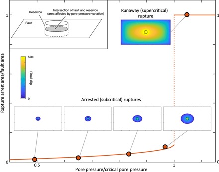
The red line and the symbols delineate the rupture arrest area as a function of pore pressure inside the perturbation. The rupture extent is also illustrated by final slip maps. The sketch in the inset depicts the relative position of a fault and a reservoir.

Fluid injection into the reservoir increases its pore pressure, which reduces the fault’s frictional strength μ_s(σ₀′ − p). A rupture nucleates if and where the fault strength drops below the shear stress. The ensuing rupture propagation is modeled with a 3D dynamic rupture simulation method (17). The typical behavior resulting from these simulations is illustrated in Fig. 1. In this example, the pore-pressure perturbation on the fault has a fixed area but increasing amplitude. To estimate an upper bound on rupture size at a given pressure, we assume that the fault is locked until that pressure is reached and then slip is released in a single event. If the pressure is low, ruptures are self-arrested. Their arrest area is significantly larger than the fluid-pressurized area. As the pressure increases, so does the rupture arrest area. When a critical pressure is reached, there is a sharp transition to runaway rupture: The rupture area jumps to a size limited only by the assumed fault boundaries. More generally, we find that whether the rupture becomes arrested or runaway depends on both the area and amplitude of the pore-pressure perturbation.

Fracture-mechanics estimates of the size of arrested ruptures

Although it is possible to conduct a parametric study of the arrest of induced earthquakes based on 3D dynamic rupture simulations, here, we develop a more efficient approach based on fracture mechanics. We validate and calibrate the approach through 3D dynamic simulations and then apply it to assess the influence of reservoir and fault parameters on the size of arrested ruptures.

To estimate the area of arrested ruptures, we apply Griffith’s crack equilibrium criterion. The criterion is essentially an energy balance equating the elastostatic energy release rate due to crack growth, G, and the fracture energy dissipated by unit of crack growth, G_c = 1/2σ′(μ_s − μ_d)D_c. To keep the derivation tractable, we approximate the rupture as circular and ignore the differences between shear crack modes (II and III). We apply known integral relations to numerically compute G(R) as a function of rupture radius R for any axisymmetric distribution of stress (21). We determine the equilibrium radii R that satisfy G(R) = G_c and apply an additional condition, d(G − G_c)/dR < 0, to identify stable equilibrium position. Finally, we use a circular crack model with uniform stress drop to compute the moment magnitude M_w from the rupture area (the derivation of the approach and its validation are presented in Materials and Methods).

Considering now an injection at a constant flow rate into a sealed reservoir, we investigate the dependency of rupture arrest area on reservoir and fault parameters. In Fig. 2A, we compare the temporal evolution of rupture arrest area for a fixed set of fault parameters (with S = 2) and for a representative range of reservoir parameters summarized in table S1. We find that the detailed distribution of pore pressure inside the reservoir is largely irrelevant: Rupture arrest area is controlled by the integral over the spatial extent of pore pressure on the fault. Consequently, reservoir parameters other than its radius do not affect the sizes of arrested ruptures, only their admissible timing. The injection rate q, fluid compressibility c_t, porosity φ, and reservoir thickness h have similar effects. At times long enough so that reservoir pressure is saturated, these parameters affect the value and temporal evolution of the average pressure but not the shape of the pressure distribution (see Fig. 3). For example, reducing injection rate q delays the onset of arrested ruptures, whereas increased injection rate leads to earlier onset, yet in both cases, the minimal and maximal rupture arrest areas are identical. On the other hand, permeability k and viscosity μ_v alter the pressure distribution but not its integral; hence, they do not affect rupture timing. Reservoir radius, r_e, is the only reservoir parameter affecting the maximum rupture size: The area of the largest arrested rupture increases with r_e (Fig. 2B).

Fig. 2. Influence of reservoir- and fault-related parameters on the evolution of rupture arrest area.

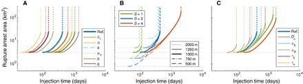
(A) Varying reservoir-related parameters, (B) varying strength parameter S and reservoir radius r_e, and (C) varying fault-related parameters. The reference solution (bold blue line) is the same in all three panels. In each panel, the same color depicts the solutions for the same varying parameter. For (A) and (C), thin and bold lines indicate solutions for lower and greater value of the corresponding parameter compared to that of the reference solution. For stresses in (C), the thin and thick lines indicate lower and higher values of S, respectively. Transition to runaway ruptures is marked by the dashed lines. The horizontal gray lines indicate the area of the intersection of the reservoir and the fault; it also corresponds to the minimal arrested area. The horizontal dotted gray line in (A) indicates constant maximum arrested area (in other panels, maximum arrested area varies). Note that in (C), the lines for τ₀ and σ are almost identical.

Fig. 3. Comparison of pore-pressure distribution inside sealed cylindrical reservoirs induced at time t = 100 days by steady-flux injection at its center, for varying compressibility c_t, viscosity μ_v, porosity φ, and permeability k.

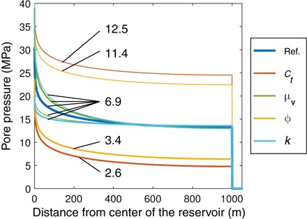
Higher and lower values of parameters are depicted by thicker and thinner lines of the same color, respectively. The numbers indicate the values of the spatial integral of pressure in megapascals per square kilometer.

The effect of fault parameters on arrested rupture area is illustrated in Fig. 2 (B and C). Fault parameters (μ_s, μ_d, D_c, τ₀, and σ) influence both the timing of the onset of arrested ruptures and the subsequent temporal evolution of the rupture arrest area. For example, faults with lower background stress τ₀ (higher S; Fig. 2B) or larger slip-weakening distance D_c (Fig. 2C) can produce larger arrested ruptures. This is expected because both smaller energy available to drive ruptures and larger fracture energy (larger fault resistance to rupture growth) tend to stabilize a fault.

Magnitude of the largest arrested rupture

The magnitude of the largest arrested rupture, ${\mathit{M}}_{\mathrm{w}}^{\text{max}-\text{arr}}$, is an important indicator of the stability of a perturbed fault. A fault capable of producing runaway ruptures is relatively unstable. Noting that the largest arrested ruptures are significantly larger than the fluid-pressurized area, we obtain further insight into what controls ${\mathit{M}}_{\mathrm{w}}^{\text{max}-\text{arr}}$ by approximating the additional stress drop (induced by the pore-pressure perturbation) as a point load superimposed on the background stress drop. This approximation leads to the following estimate of the maximum arrested moment (see Eqs. 19 and 21)

$${\mathit{M}}_0^{\text{max}-\text{arr}}=0.4255{\mathrm{\Delta }\mathrm{\tau }}_0{\left(\frac{{\mathrm{\mu }}_{\mathrm{d}}\cdot \mathrm{\Delta }\mathit{p}\cdot {\mathit{A}}_{\mathit{p}}}{{\mathrm{\Delta }\mathrm{\tau }}_0}\right)}^{\raisebox{1ex}{$3$}\!\left/ \!\raisebox{-1ex}{$2$}\right.}$$ (1)

where Δp is the average increase in pore pressure inside the reservoir, A_p is the area of the stress perturbation (here, the area of intersection between the reservoir and the fault), μ_d is the dynamic friction coefficient, and Δτ₀ is the background stress drop. The corresponding moment magnitude ${\mathit{M}}_{\mathrm{w}}^{\text{max}-\text{arr}}$ is computed using Eq. 20.

The result in Eq. 1 reflects how rupture arrest is controlled by a competition between two sources of elastic energy: injection-induced fluid pressure and tectonic prestress. The contributions of these two sources to the elastic energy available for rupture growth (via the stress intensity factor in Eq. 18) are both positive. However, the energy contributed by injection-induced fluid pressure decays with increasing rupture size, whereas the energy contributed by tectonic prestress increases, thereby creating a trade-off between these two strain-energy sources. At the maximum arrest size, both contributions are comparable. Hence, although arrested ruptures can grow well beyond the reservoir boundaries, the reservoir pressure not only triggers them but also contributes significantly to their energy balance.

To draw the connection between ${\mathit{M}}_0^{\text{max}-\text{arr}}$ and injection parameters, following McGarr (9), we approximate the average increase in pore pressure after injecting a volume ΔV of fluid into a saturated reservoir of volume V as

$$\mathrm{\Delta }\mathit{p}=\mathrm{\kappa }\frac{\mathrm{\Delta }\mathit{V}}{\mathit{V}}$$ (2)

where κ is the bulk modulus of the reservoir rock. This approximation assumes an incompressible fluid and neglects the effects of porosity on the ability of a rock formation to accommodate fluid pressure diffusion or distribution. For the scenario of Fig. 1, the volume affected by the stress perturbation is V = A_p⋅h, where h is the reservoir thickness, and Eqs. 1 and 2 yield

$${\mathit{M}}_0^{\text{max}-\text{arr}}=\mathrm{\gamma }\cdot \mathrm{\Delta }{\mathit{V}}^{\raisebox{1ex}{$3$}\!\left/ \!\raisebox{-1ex}{$2$}\right.} \text{where} \mathrm{\gamma }\doteq \frac{0.4255}{\sqrt{{\mathrm{\Delta }\mathrm{\tau }}_0}}{\left(\frac{\mathrm{\kappa }\cdot {\mathrm{\mu }}_{\mathrm{d}}}{\mathit{h}}\right)}^{\raisebox{1ex}{$3$}\!\left/ \!\raisebox{-1ex}{$2$}\right.}$$ (3)

We note that, for example, a greater stress drop Δτ₀ leads to smaller values of ${\mathit{M}}_0^{\text{max}-\text{arr}}$, reflecting the fact that transition to runaway ruptures will occur earlier for a fault with a greater stress drop than for a fault with a lower stress drop. Comparison to computations accounting for the exact stress drop distribution in ~4250 randomly generated reservoir-fault configurations (see Materials and Methods) shows that the point-load approximation of ${\mathit{M}}_{\mathrm{w}}^{\text{max}-\text{arr}}$ is unbiased and accurate within an uncertainty of ±0.5. More generally, the term F = μ_d ⋅ Δp ⋅ A_p in Eq. 1 can be interpreted as the spatial integral of a localized perturbation of potential stress drop resulting from the intersection of a fault with a fluid-pressurized volume or a poroelastic stress distribution or from pressure diffusion along a permeable fault zone channel.

In Fig. 4, we compare our ${\mathit{M}}_{\mathrm{w}}^{\text{max}-\text{arr}}$ estimates with the largest magnitudes observed in various injection-induced earthquake sequences as a function of the cumulative net injected fluid volumes in nearby wells. We consider three values of γ corresponding to plausible values of key model parameters (h from 10 to 1000 m, Δτ₀ from 0.1 to 10 MPa, κ = 50 GPa, and μ_d = 0.1). An induced earthquake with magnitude below our predicted ${\mathit{M}}_{\mathrm{w}}^{\text{max}-\text{arr}}$ is interpreted as a spontaneously arrested rupture. Because moment can be accommodated by aseismic slip or by multiple earthquakes on the same fault, ${\mathit{M}}_{\mathrm{w}}^{\text{max}-\text{arr}}$ is a conservative upper magnitude bound for arrested ruptures. Conversely, an earthquake with magnitude above our predicted ${\mathit{M}}_{\mathrm{w}}^{\text{max}-\text{arr}}$ is interpreted as a runaway rupture. In reality, arrested ruptures are likely to stop even before they reach their maximum size because even small or weak barriers can significantly affect their propagation. A runaway rupture needs a stronger and larger barrier to be stopped, typically the end of a fault or a geometrical/geological fault segmentation. In this context, larger values of γ and ${\mathit{M}}_{\mathrm{w}}^{\text{max}-\text{arr}}$ lead to a more stable situation.

Fig. 4. Comparison of our estimate of magnitude of maximum arrested rupture, ${\mathit{M}}_{\mathrm{w}}^{\text{max}-\text{arr}}$, for three values of γ with magnitudes of injection-induced earthquakes over a broad range of injected volumes.

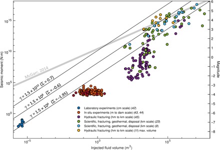
We find that our estimate is equivalent to that of magnitude of maximum possible earthquake by van der Elst et al. (12) for b = 1; therefore, we also indicate the corresponding values of seismogenic index A_p. For completeness, we also include the estimate of maximum possible induced earthquake by McGarr (9). Note that for the events induced during multistage hydrofracking in the Western Canada sedimentary basin (yellow circles), we consider the total volumes for all previous stages and all proximal well completions reported as “maximum volume” by Atkinson et al. (11).

Figure 4 reveals a striking consistency between the relation ${\mathit{M}}_0^{\text{max}-\text{arr}}\propto \mathrm{\Delta }{\mathit{V}}^{\raisebox{1ex}{$3$}\!\left/ \!\raisebox{-1ex}{$2$}\right.}$ predicted by our model and data recorded across a very broad range of injected volumes and scales, from laboratory experiments (centimeter scale) to induced seismicity at field scales (hectometers to kilometers), including intermediate-scale natural laboratories (meters to dekameters). Moreover, almost all magnitudes fall below the predicted ${\mathit{M}}_{\mathrm{w}}^{\text{max}-\text{arr}}$, with γ = 1.5 × 10¹⁰. These two observations suggest that these induced earthquakes may have been arrested ruptures.

DISCUSSION

Our model does not provide an estimate of maximum possible magnitude M_max, only the maximum size of arrested ruptures ${\mathit{M}}_{\mathrm{w}}^{\text{max}-\text{arr}}$. Ruptures can grow larger if they are runaway. It is nevertheless informative to compare it with previous estimates of M_max of injection-induced earthquakes.

McGarr (9) proposed a linear relation between M_{0 max} and ΔV, which differs significantly from our physics-based prediction ${\mathit{M}}_0^{\text{max}-\text{arr}}\propto \mathrm{\Delta }{\mathit{V}}^{\raisebox{1ex}{$3$}\!\left/ \!\raisebox{-1ex}{$2$}\right.}$. Although for low injected volumes, McGarr’s model largely overpredicts observed maximum magnitudes, several cases from data sets by Buijze et al. (23) and Atkinson et al. (11) exceed his model for large injected volumes. Our model is more consistent with the data as a whole; however, the difference between our model and maximum observed magnitudes increases with injected fluid volume, suggesting that fluid injection can induce even larger events than what has been recorded so far. This difference concerns magnitudes >4 and is therefore significant for seismic hazard analysis.

Comparing ${\mathit{M}}_{\mathrm{w}}^{\text{max}-\text{arr}}$ with the estimate ${\widehat{\mathit{M}}}_{\mathit{w}}^{\text{max}}$ by van der Elst et al. (12), based on the premise that induced seismicity is Poissonian and follows the Gutenberg-Richter magnitude-frequency distribution, like regular tectonic earthquakes, reveals interesting similarities. Their model predicts ${\widehat{\mathit{M}}}_0^{\text{max}}\propto \mathrm{\Delta }{\mathit{V}}^{\raisebox{1ex}{$3$}\!\left/ \!\raisebox{-1ex}{$2\mathit{b}$}\right.}$, where b is the Gutenberg-Richter exponent. If b = 1, both models predict exponent of ³/₂. Equating the prefactors, the seismogenic index Σ of their model can be related to our parameter γ by $\mathrm{\Sigma }=\frac{2}{3}{\text{log}}_{10}\mathrm{\gamma }-6.07$. The range of γ values in Fig. 4 yields a reasonable range of values of Σ. Because ${\widehat{\mathit{M}}}_{\mathit{w}}^{\text{max}}$ estimates maximum magnitude and our ${\mathit{M}}_{\mathrm{w}}^{\text{max}-\text{arr}}$ estimates the largest arrested rupture, the similarity between the two estimates is unexpected. For b ≠ 1 (b > 1 is common for induced seismicity), the two models no longer yield consistent results. Using our terminology, van der Elst et al. (12) showed that runaway ruptures that stopped because of natural heterogeneity of tectonic stresses are a viable explanation of the M_max versus injected volume data. Our model allows both possibilities (the largest observed ruptures could be either runaway or self-arrested), and we show that the latter is viable too. However, our attempts to discriminate the two models by their predictions of the relative timing of the largest earthquake are inconclusive because of the scarcity of data (see Materials and Methods).

Our analysis shows that rupture arrest and the transition to runaway rupture are dominantly controlled by friction parameters and stress state (that is, conditions on the fault before injection), whereas the temporal evolution of pore pressure only influences timing (that is, triggering). Our model also reveals that for the same pore pressure, a larger reservoir can produce larger events than a smaller reservoir. This implies that there is no universal safe pressure limit; what matters is the product F = μ_d ⋅ Δp ⋅ A_p. This also explains, conceptually, how low-pressure wastewater disposal into an extended reservoir may induce larger events than hydrofracking operations involving higher pore pressure but over a smaller footprint.

Our model also reveals significant variations in the duration of the relatively stable, arrested rupture regime. This may have important implications for traffic-light systems (TLSs) aiming at operational control of induced earthquake hazard. A TLS that implicitly assumes that magnitudes of induced earthquakes do not change abruptly with time or a TLS with magnitude thresholds higher than ${\mathit{M}}_{\mathrm{w}}^{\text{max}-\text{arr}}$ could fail to capture an abrupt transition to runaway ruptures. In the framework of our model, a TLS may be particularly challenged in reservoir-fault systems characterized by a short arrested rupture regime.

Although our scaling of ${\mathit{M}}_0^{\text{max}-\text{arr}}$ with injected volume has been derived for the point-force approximation of the injection scenario captured in Fig. 1, we believe that it is more robust and applicable to a wider range of scenarios. Strictly speaking, the point-force approximation is valid if the pressurized region is small compared to the size of the maximum arrested rupture. However, the verification of the point-force approximation using the finite-reservoir approach revealed that the point-force approximation is robust, as demonstrated by no systematic correlation of residuals with other fault-reservoir parameters (fig. S6), particularly with strength parameter S (from 1.5 to 8), radius of reservoir (from 0.1 to 5 km), or magnitudes (from 4 to 8). The only exceptions are compressibility and porosity, whose effects, as discussed, are neglected in the approximation of the average pore pressure (Eq. 2). Moreover, our approach can be applied to more general injection scenarios than depicted in Fig 1. For example, if an arbitrarily oriented fault intersects a general-shaped reservoir, the resulting scaling remains ${\mathit{M}}_0^{\text{max}-\text{arr}}\propto \mathrm{\Delta }{\mathit{V}}^{\raisebox{1ex}{$3$}\!\left/ \!\raisebox{-1ex}{$2$}\right.}$, but reservoir thickness h in the parameter γ is replaced by the ratio of volume of the reservoir and the area of the intersection, V/A_p. For a special case of a vertical fault intersecting a cylindrical reservoir at distance D from the reservoir center, $\mathit{V}/{\mathit{A}}_{\mathit{p}}=\mathrm{\pi }{\mathit{R}}^2/(2\sqrt{{\mathit{R}}^2-{\mathit{D}}^2})$.

Beyond injection-induced seismicity, our theory for rupture arrest is potentially applicable to faults loaded by localized stresses of other origins, which can be represented by an effective load F, including situations that are relevant for natural seismicity. For instance, F could arise from stochastic stresses (21) or from stress concentrations due to localized fault loading (19). In particular, creep in the deep extension of a fault concentrates stress at the base of the seismogenic zone. In earthquake cycle simulations, this loading nucleates sequences of arrested ruptures at a depth before a runaway rupture. Megathrust earthquakes that remained confined at depth, like the 2015 Gorkha, Nepal earthquake (24, 25), may be examples of these arrested ruptures, a necessary prelude to a much larger event. The belt of background seismicity in Nepal is consistent with concentrated tectonic loading around the bottom of the megathrust seismic coupling zone. The appropriateness of one of our key model assumptions, the Griffith’s fracture criterion, for natural earthquake arrest is supported by microseismicity observations. On strike-slip faults, the criterion predicts that rupture arrest length is larger horizontally (mode II) than vertically (mode III) by a factor 1/(1 − ν), where ν is the Poisson’s ratio. This is consistent with the aspect ratio of rupture areas inferred from aftershocks of microearthquakes in California (26).

Although our approach allows scaling of fracture energy with rupture size, here, we assumed constant fracture energy on each rupture. Considering an empirical model (27) and a thermal pressurization model (28) of fracture energy scaling with slip, which both fit the relevant seismological observations adequately, we find qualitatively different results for rupture arrest size. Thus, further study of earthquake arrest can help advance our understanding of fracture energy scaling.

MATERIALS AND METHODS

Pore pressure in a cylindrical reservoir

We used the general solution of the diffusion equation for single-phase fluid flow for a cylindrical reservoir, with constant injection rate at its center and no-flow boundary condition [Appendix B in the study of Lee et al. (29)]. The dimensionless diffusion equation exploiting axisymmetry is

$$\frac{1}{{\mathit{r}}_{\mathrm{D}}}\frac{\partial }{\partial {\mathit{r}}_{\mathrm{D}}}\left({\mathit{r}}_{\mathrm{D}}\frac{\partial {\mathit{p}}_{\mathrm{D}}}{\partial {\mathit{r}}_{\mathrm{D}}}\right)=\frac{\partial {\mathit{p}}_{\mathrm{D}}}{\partial {\mathit{t}}_{\mathrm{D}}}$$ (4)

where r_D = r/r_w is the dimensionless radius (r being the radius and r_w being the wellbore radius)

$${\mathit{t}}_{\mathrm{D}}=\frac{\mathit{t}\cdot \mathit{k}}{\mathrm{\phi }\cdot {\mathrm{\mu }}_{\mathrm{v}}\cdot {\mathit{c}}_{\mathit{t}}\cdot {\mathit{r}}_{\mathrm{w}}^2}$$ (5)

is the dimensionless time (t being the time, k and φ being the permeability and porosity of the reservoir, respectively, and c_t being the compressibility of the fluid), and

$${\mathit{p}}_{\mathrm{D}}=\frac{2\mathrm{\pi }\cdot \mathit{k}\cdot \mathit{h}}{\mathit{q}\cdot \mathit{B}\cdot {\mathrm{\mu }}_{\mathrm{v}}}({\mathit{p}}_{\mathrm{i}}-\mathit{p})$$ (6)

is the dimensionless pressure (h being the reservoir height, q being the injection rate (negative sign indicates withdrawal), B being the formation volume factor, μ_v being the fluid viscosity, p_i being the initial pore pressure, and p being the current pore pressure). The initial condition is

$${\mathit{p}}_{\mathrm{D}}({\mathit{r}}_{\mathrm{D}},{\mathit{t}}_{\mathrm{D}}=0)=0$$ (7)

the inner boundary condition (that is, constant injection rate) is given as

$${\left({\mathit{r}}_{\mathrm{D}}\frac{\partial {\mathit{p}}_{\mathrm{D}}}{\partial {\mathit{r}}_{\mathrm{D}}}\right)}_{{\mathit{r}}_{\mathrm{D}}=1}=-1$$ (8)

whereas the outer boundary condition (that is, no-flow boundary) is given as

$${\left(\frac{\partial {\mathit{p}}_{\mathrm{D}}}{\partial {\mathit{r}}_{\mathrm{D}}}\right)}_{{\mathit{r}}_{\mathrm{D}}={\mathit{r}}_{\text{eD}}}=0$$ (9)

where r_eD = r_e/r_w is dimensionless radius of the reservoir. The general solution for r_D ≤ r_eD and t_D ≥ 0 is

$${\mathit{p}}_{\mathrm{D}}({\mathit{r}}_{\mathrm{D}},{\mathit{t}}_{\mathrm{D}})=\frac{2}{{\mathit{r}}_{\text{eD}}^2-1}(\frac{{\mathit{r}}_{\mathrm{D}}^2}{4}+{\mathit{t}}_{\mathrm{D}})-\frac{{\mathit{r}}_{\text{eD}}^2\cdot \text{ln} {\mathit{r}}_{\mathrm{D}}}{{\mathit{r}}_{\text{eD}}^2-1}-\frac{3{\mathit{r}}_{\text{eD}}^4-4{\mathit{r}}_{\text{eD}}^4\cdot \text{ln} {\mathit{r}}_{\text{eD}}-2{\mathit{r}}_{\text{eD}}^2-1}{4{({\mathit{r}}_{\text{eD}}^2-1)}^2}+\mathrm{\pi }{\displaystyle \sum _{\mathit{n}=1}^{\infty }}{\mathrm{\Psi }}_{\mathit{n}}({\mathit{r}}_{\mathrm{D}}){\mathrm{e}}^{-{\mathrm{\alpha }}_{\mathit{n}}^2\cdot {\mathit{t}}_{\mathrm{D}}}{\mathit{J}}_1^2({\mathrm{\alpha }}_{\mathit{n}}{\mathit{r}}_{\text{eD}})$$ (10)

where J_k and Y_k are the kth-order Bessel functions of the first and second kind, respectively

$${\mathrm{\Psi }}_{\mathit{n}}({\mathit{r}}_{\mathrm{D}})=\frac{{\mathit{J}}_1({\mathrm{\alpha }}_{\mathit{n}}){\mathit{Y}}_0({\mathrm{\alpha }}_{\mathit{n}}{\mathit{r}}_{\mathrm{D}})-{\mathit{Y}}_1({\mathrm{\alpha }}_{\mathit{n}}){\mathit{J}}_0({\mathrm{\alpha }}_{\mathit{n}}{\mathit{r}}_{\mathrm{D}})}{{\mathrm{\alpha }}_{\mathit{n}}({\mathit{J}}_1^2({\mathrm{\alpha }}_{\mathit{n}}{\mathit{r}}_{\text{eD}})-{\mathit{J}}_1^2({\mathrm{\alpha }}_{\mathit{n}}))}$$ (11)

and α_n(r_eD) is the nth root of the equation

$${\mathit{J}}_1({\mathrm{\alpha }}_{\mathit{n}}{\mathit{r}}_{\text{eD}})\cdot {\mathit{Y}}_1({\mathrm{\alpha }}_{\mathit{n}})-{\mathit{J}}_1({\mathrm{\alpha }}_{\mathit{n}})\cdot {\mathit{Y}}_1({\mathrm{\alpha }}_{\mathit{n}}{\mathit{r}}_{\text{eD}})=0$$ (12)

The last term in the p_D solution (Eq. 10) is a transient component that vanishes at long times.

Estimation of rupture arrest area

We derived estimates of the rupture arrest area given a spatial distribution of potential stress drop, Δτ, based on the Griffith crack equilibrium criterion and small-scale yielding fracture mechanics. Following the approach in Appendix B in the study of Ripperger et al. (21) and Appendix A in the study of Galis et al. (17), we adopted the following simplifying assumptions:

(1) The rupture is approximately circular, with radius R.

(2) The stress drop distribution is axisymmetric, Δτ(r).

(3) The static stress intensity factor averaged along the crack rim is approximated by the expression for tensile (mode I) cracks

$${\mathit{K}}_0(\mathit{R})=\frac{2}{\sqrt{\mathrm{\pi }\mathit{R}}}{\displaystyle {\int }_0^{\mathit{R}}}\frac{\mathrm{\Delta }\mathrm{\tau }(\mathit{r})}{\sqrt{{\mathit{R}}^2-{\mathit{r}}^2}}\mathit{r}\mathit{d}\mathit{r}$$ (13)

(4) The details of weakening inside the process zone are ignored, and the rupture criterion is based on the fracture toughness K_c, related to the slip-weakening fracture energy by

$${\mathit{G}}_{\mathrm{c}}=\frac{1}{2}({\mathrm{\tau }}_{\mathrm{s}}-{\mathrm{\tau }}_{\mathrm{d}}){\mathit{D}}_{\mathrm{c}}=\frac{1}{2\mathrm{\mu }}{\mathit{K}}_{\mathrm{c}}^2$$ (14)

Although we considered here a slip-weakening model with constant G_c, a scale-dependent G_c(R) can be incorporated too. The conditions for rupture arrest are

$${\mathit{K}}_0(\mathit{R})={\mathit{K}}_{\mathrm{c}} \text{and} \frac{\partial ({\mathit{K}}_0-{\mathit{K}}_{\mathrm{c}})}{\partial \mathit{R}}<0$$ (15)

The first condition is the Griffith’s crack equilibrium criterion, and the second condition is necessary to find a stable equilibrium at which further perturbation does not lead to further self-accelerating dynamic rupture. Galis et al. (17) considered an adjustable factor η in the Griffith’s criterion, that is, η ⋅ K₀(R) = K_c, as a proxy to account for the differences between modes I, II, and III, the departures from circularity, the effect of dynamic overshoot, etc. They found that η = 1 yields results consistent with numerical simulations; therefore, we adopted η = 1. In numerical simulations, the stresses in the hypocentral area were chosen so that the initial condition was near an unstable equilibrium state (∂(K₀ − K_c)/∂R > 0).

The solution of the problem (15) was found by numerically integrating K₀(R) (Eq. 13) with adaptive sampling of R and r to achieve high accuracy of the rupture arrest radius, R_arr, for various stress drop distributions. The rupture arrest area was then obtained as ${\mathit{A}}_{\text{arr}}=\mathrm{\pi }{\mathit{R}}_{\text{arr}}^2$. If a solution to Eq. 15 exists, it represents the final radius R of an arrested rupture. Otherwise, rupture is runaway.

We considered stress drop distributions with identical peak amplitude such that τ₀ > τ_s at r = 0 but with varying width (Fig. 5). Such a peak could result from reduced normal stress due to locally increased pore pressure. The stress drop perturbation affects the shape of K₀(R) following three cases depending on its width. If the perturbation is too narrow, rupture does not propagate outside the overstressed area because the perturbed K₀ does not reach K_c. If the perturbation is large enough, it initiates a runaway rupture because, once K₀ becomes greater than K_c, it will remain greater. In the intermediate case, rupture starts propagating outside the overstressed region, but the rupture eventually stops when the stable equilibrium is reached, that is, K₀ = K_c on the decreasing leg of K₀.

Fig. 5. Fracture mechanics of rupture arrest under nonuniform stress.

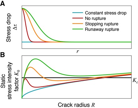
Sketch of (A) stress drop distributions Δτ(r) and (B) the corresponding static stress intensity factors K₀(R) illustrating different crack behavior (although our approach supports K_c being a function of R, for illustration purposes, K_c is plotted as a constant).

We obtained further physical insight by developing a simplified analytical estimate. For this purpose, we assumed that K_c is constant and the rupture arrest area is much larger than the fluid-pressurized area A_p. Following the study of Galis et al. (17), we approximated stress drop by a point load superimposed on the background uniform stress drop

$$\mathrm{\Delta }\mathrm{\tau }(\mathit{r})\doteq \mathrm{\Delta }{\mathrm{\tau }}_0+\mathit{F}\cdot \mathrm{\delta }(\mathit{r})/(2\mathrm{\pi }\mathit{r})$$ (16)

where

$$\mathit{F}={\mathrm{\mu }}_{\mathrm{d}}\cdot \mathrm{\Delta }\mathit{p}\cdot {\mathit{A}}_{\mathit{p}}$$ (17)

Here, Δp is the average increase in pore pressure inside the reservoir. We adopted a definition of Dirac’s distribution in polar coordinates consistent with ${\displaystyle {\int }_0^{\mathit{R}}}\mathrm{\delta }(\mathit{r})\mathit{r}\cdot \mathit{d}\mathit{r}=1$ (30). After inserting Eq. 16 into Eq. 13, we obtained

$${\mathit{K}}_0(\mathit{R})=\frac{\mathit{F}}{{(\mathrm{\pi }\mathit{R})}^{\raisebox{1ex}{$3$}\!\left/ \!\raisebox{-1ex}{$2$}\right.}}+2\mathrm{\Delta }{\mathrm{\tau }}_0\sqrt{\frac{\mathit{R}}{\mathrm{\pi }}}$$ (18)

Solving the Griffith’s equilibrium condition (Eq. 15) leads to a quartic equation with too complicated solutions to provide the desired insight. Yet, a compact expression can be derived for the maximum rupture arrest radius, R_{max − arr}. The first term of Eq. 18 decreases with R, whereas the second term increases; hence, K₀(R) has a single minimum. Runaway ruptures are possible only if this minimum exceeds K_c because, then, the Griffith’s equilibrium criterion cannot be satisfied for any R. The rupture radius at the minimum of K₀ gives

$${\mathit{R}}_{\text{max}-\text{arr}}=\sqrt{\frac{3\cdot \mathit{F}}{2\mathrm{\pi }\cdot \mathrm{\Delta }{\mathrm{\tau }}_0}}=\sqrt{\frac{3\cdot {\mathrm{\mu }}_{\mathrm{d}}\cdot \mathrm{\Delta }\mathit{p}\cdot {\mathit{A}}_{\mathit{p}}}{2\mathrm{\pi }\cdot \mathrm{\Delta }{\mathrm{\tau }}_0}}$$ (19)

The corresponding rupture arrest area is ${\mathit{A}}_{\text{max}-\text{arr}}=\mathrm{\pi }\cdot {\mathit{R}}_{\text{max}-\text{arr}}^2$.

Verification of theoretical estimates of rupture arrest area

We verified our theoretical estimates of rupture arrest area by comparison with 3D dynamic rupture simulations. First, we analyzed results for a step-like distribution of stress drop with Δτ(r) = Δτ_i for r ≤ R_i and Δτ(r) = Δτ₀ for r > R_i. Galis et al. (17) performed dynamic rupture simulations on a 30 × 15–km fault with μ_s = 0.6778, μ_d = 0.525, d_c = 0.4 m, and σ = 120 MPa and various values of strength parameter S (obtained by varying τ₀) to investigate conditions for runaway ruptures. The fault is large enough so that ruptures that break the entire fault are considered runaway ruptures. Here, we considered the same configurations. Figure 6A shows very good agreement between estimated and simulated rupture arrest areas for all considered values of S and R_i, including the transition to runaway ruptures. The comparison further revealed that our approach worked equally well for circular, elliptical, and square perturbations, although it was based on an assumption of radially symmetric stress drop. To achieve agreement between theory and numerical results, we introduced a correction factor ϕ = 2 such that ${\mathit{A}}_{\text{arr}}^{\text{num}}=\mathrm{\varphi }{\mathit{A}}_{\text{arr}}$ or ${\mathit{R}}_{\text{arr}}^{\text{num}}=\sqrt{\mathrm{\varphi }}{\mathit{R}}_{\text{arr}}$. Galis et al. (17) introduced an adjustable factor η multiplying K₀ to account for deviations from circular mode I rupture. The factor ϕ introduced here has a different role; it accounts for the effects affecting crack radius R. In terms of the K₀(R) plot in Fig. 5B, η provides a correction for the y axis, whereas ϕ provides a correction for the x axis.

Fig. 6. Verification of our theoretical estimates with numerical results.

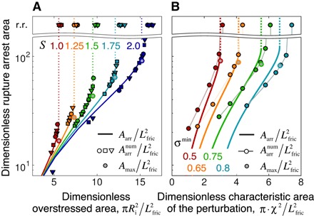
Comparison of estimated rupture arrest area A_arr and maximum rupture arrest area A_max with rupture arrest area from numerical simulations ${\mathit{A}}_{\text{arr}}^{\text{num}}$ as functions of overstressed area for (A) a steplike distribution of stress drop and varying strength parameter S (B), a Gaussian distribution of stress drop, and varying minimal normal stress σ^min. For a step-like stress drop distribution, we performed simulations with circular, square, and elliptical perturbations marked by circles, squares, and triangles. The transitions from solid to dashed lines indicate transition from arrested to runaway ruptures. The undulated double line indicates interrupted y axis; r.r. indicates runaway ruptures. L_fric = μ ⋅ D_c/(τ_s0 − τ_d0) is a characteristic length scale introduced by the slip-weakening process (39).

Next, we analyzed results for stress drop with a Gaussian perturbation, Δτ(r) = Δτ₀ + μ_dσ₀′(1 − σ^min) ⋅ exp(−r²/(2 χ²)), as would result from an instantaneous pressure point source at r = 0 (31). We adopted the same friction parameters as those of Galis et al. (17), yielding Δτ₀ = 6.1 MPa, and considered σ^min = 0.5, 0.65, 0.75, and 0.8. Figure 6B shows the overall consistency between estimated and simulated rupture arrest areas as a function of the characteristic area of the stress perturbation, πχ². Part of the small differences decrease with mesh refinement (fig. S1) and are attributed to the staircase representation of the smooth stress drop distribution in a discrete grid. For the larger σ^min values considered, the critical perturbation area at the transition to runaway ruptures was underestimated. This was expected because our theoretical estimates lacked a rupture nucleation criterion to account for the finite size of the initiation area (where the initial stress is higher than the static strength).

Figure 6 also shows very good agreement between theory and numerical results for the maximum area of spontaneously arrested ruptures, A_max. The agreement improved with increasing S for the steplike stress drop and with decreasing σ^min for the Gaussian distribution because in this case, the assumptions for the point-load approximation were better satisfied (fig. S2). Although both examples represent spatially variable stress drop and nucleation of ruptures by increased fluid pressure, the results for step-like distributions are more relevant for a sealed reservoir.

Conversion of rupture arrest size to magnitude

Moment magnitude M_w is defined by (32)

$${\mathit{M}}_{\mathrm{w}}=\frac{2}{3} {\text{log}}_{10}{\mathit{M}}_0-6.07$$ (20)

where M₀ is the seismic moment. We derived the seismic moment from the initial stress information using the equation for a circular crack with uniform stress drop (33)

$${\mathit{M}}_0=\frac{16}{7}{\mathrm{\Delta }\mathrm{\tau }}_0{\mathit{R}}^3$$ (21)

Strictly speaking, the formula should be based on the static stress drop, which differs from the dynamic stress drop Δτ₀ due to dynamic overshoot. The average dynamic and static stress drops of arrested ruptures are almost identical (fig. S3), and in highly heterogeneous ruptures, they differ by only 10% on average (34). Because the pressurized region is small compared to the rupture area, we approximated the average stress drop as Δτ₀, neglecting the additional stress drop μ_d ⋅ Δp inside the reservoir. Figure S4 compares magnitudes estimated by this approach with those obtained from dynamic rupture simulations by directly applying the definition of seismic moment

$${\mathit{M}}_0=\mathrm{\mu }{\displaystyle \mathrm{\int }\mathrm{\int }}\mathit{D}\mathit{d}{\mathit{x}}^2$$ (22)

where μ is the shear modulus, and D is the final slip. Rupture simulations were initiated artificially by prescribing an area in which the initial stress slightly exceeded the static frictional strength. We excluded this initiation area from the magnitude computation because it contained artificially large slip. Overall, for rupture areas from 1 to 500 km², the approximation to M_w using Eq. 21 agrees with the numerical simulation results, with deviations smaller than ~0.1 and insignificant underestimation. It is also naturally consistent with empirical scaling relations based on the self-similar rupture model, in particular, with the relation for stable continental regions by Leonard (35), which assumes a stress drop value (5.84 MPa) that is very similar to the background stress drop in our simulations (6.11 MPa).

Verification of point-load approximation of reservoir

Here, we verified the adequacy of the maximum arrested rupture magnitude estimated under the point-load approximation, ${\mathit{M}}_{\mathrm{w}}^{\text{max}-\text{arr}}$. We considered ~4250 randomly generated reservoir-fault configurations. Values of reservoir parameters (that is, viscosity, permeability, compressibility, porosity, well radius, flow rate, height, and radius of the reservoir) were sampled as independent, uniformly distributed variables within ranges reported for common reservoirs (36, 37). The following fault-related parameters were sampled from uniform distributions: μ_s, μ_d/μ_s, depth, and S. Normal background stress was derived from depth assuming a typical density of shallow crust and water (2500 and 1000 kg m⁻³, respectively). To improve the sampling of lower magnitudes events, we increased the number of models with lower S, reservoir radius, and D_c, the only three parameters that exhibited signs of correlation with magnitude. Histograms of model parameters are shown in fig. S5. For each parameter setting, we computed the exact value of the maximum arrested earthquake magnitude, ${\mathit{M}}_{\mathrm{w}}^{\text{crit}}$, by numerically solving the rupture arrest conditions accounting completely for the finite size of the reservoir. Correlation plots between model parameters and ${\mathit{M}}_{\mathrm{w}}^{\text{crit}}$ are shown in fig. S6.

Figure S7 reveals good agreement between the point-load approximation (${\mathit{M}}_{\mathrm{w}}^{\text{max}-\text{arr}}$) and the finite-reservoir calculation (${\mathit{M}}_{\mathrm{w}}^{\text{crit}}$). Scatter was expected because of the approximation of the average reservoir pore pressure Δp (Eq. 2). In particular, the approximation neglects the effects of compressibility and effects of porosity on the ability of a formation to accommodate fluid. Both assumptions lead to systematic deviation of Δp from the true average pore pressure, which was also manifested by the weak correlation of compressibility and porosity with residuals (fig. S6). The scatter of ${\mathit{M}}_{\mathrm{w}}^{\text{max}-\text{arr}}$ is mostly confined within ±0.5, with only few points reaching down to −1. This indicates that the influence of compressibility and porosity is not strong enough to cause a significant deviation of ${\mathit{M}}_{\mathrm{w}}^{\text{max}-\text{arr}}$ from ${\mathit{M}}_{\mathrm{w}}^{\text{crit}}$. The approximation of Δp also neglects the effects of viscosity and permeability, but as shown in Fig. 3, these parameters affect the pressure distribution without affecting the average pressure. The nonsymmetric distribution of the orthogonal residuals has mean and median close to zero (− 0.13 and − 0.1, respectively). We concluded that ${\mathit{M}}_{\mathrm{w}}^{\text{max}-\text{arr}}$ is consistent with ${\mathit{M}}_{\mathrm{w}}^{\text{crit}}$ with uncertainty ±0.5.

Predictions of the relative timing of the largest earthquake

In the model by van der Elst et al. (12), the probability of occurrence of the largest earthquake is uniformly distributed within a sequence. In our model, the potential size of arrested ruptures grows with ongoing injection; hence, the largest triggered event has a higher chance to occur later in the sequence. However, our model does not make a specific prediction about how strong this tendency is; its effect could be a slight increase of probability with time. Moreover, the induced seismicity sequences considered by van der Elst et al. (12) contain also aftershocks of the largest event, which tends to bias low the rank of occurrence of the largest event.

We applied the two-sample Anderson-Darling (AD) test (38) to assess whether the occurrence rank of the largest event in the recorded induced sequences is drawn from each of the following three distributions: uniform, linearly increasing, and Gaussian (the latter being a proxy for a distribution biased by aftershocks). For the linear and Gaussian distributions, we determined optimal parameters by grid search to minimize the AD test statistic. Comparison of the optimal AD test values showed that all three considered distributions can explain the data with similar level of statistical significance and, therefore, none of them can be rejected (fig. S8). Consequently, our model qualitatively explains this data similarly well as the model proposed by van der Elst et al. (12). However, the current data set is small (only 17 sequences), and a larger data set may facilitate the discrimination between models in the future.

SUPPLEMENTARY MATERIALS

Supplementary material for this article is available at http://advances.sciencemag.org/cgi/content/full/3/12/eaap7528/DC1

fig. S1. Comparison of dimensionless rupture arrest area calculated from numerical simulations with grid spacing h = 50 m (circles) and h = 100 m (squares) with our theoretical estimates (bold lines) for varying σ^min (indicated by color).

fig. S2. Comparison of stress drop distributions as functions of dimensionless crack radius at the time of ${\mathit{A}}_{\text{arr}}^{\text{max}}$ for situations from Fig. 6.

fig. S3. Scaling of mean static and dynamic stress drops in results of numerical simulations.

fig. S4. Comparison of various approaches to estimate M_w from ruptured area A_arr.

fig. S5. Distributions of reservoir-fault parameters for all ~4250 configurations used for verification of ${\mathit{M}}_{\mathit{w}}^{\text{max}}$ (point-load approximation) against ${\mathit{M}}_{\mathrm{w}}^{\text{crit}}$ (finite-reservoir approach).

fig. S6. Distributions of reservoir-fault parameters for all ~4250 configurations used for verification of ${\mathit{M}}_{\mathit{w}}^{\text{max}}$ (point-load approximation) against ${\mathit{M}}_{\mathrm{w}}^{\text{crit}}$ (finite-reservoir approach).

fig. S7. Comparison of ${\mathit{M}}_{\mathrm{w}}^{\text{max}\mathit{-}\text{arr}}$ (derived for a point-load approximation of a reservoir) with ${\mathit{M}}_{\mathrm{w}}^{\text{crit}}$ (derived for a finite reservoir) and corresponding orthogonal residuals.

fig. S8. Evaluation of the probability of occurrence rank of the largest event within a sequence.

table S1. Reservoir and fault parameters used to prepare Fig. 2.

References (40, 41)

REFERENCES AND NOTES

- 1.Ellsworth W. L., Injection-induced earthquakes. Science 341, 1225942 (2013). [DOI] [PubMed] [Google Scholar]
- 2.Elsworth D., Spiers C. J., Niemeijer A. R., Understanding induced seismicity. Science 354, 1380–1381 (2016). [DOI] [PubMed] [Google Scholar]
- 3.Building Seismic Safety Council (BSSC), “NEHRP recommended seismic provisions for new buildings and other structures” (Report No. FEMA P-1050-1/2015 Edition, National Institute of Building Sciences, 2015); www.nibs.org/?page=bssc_pubs.
- 4.Thingbaijam K. K. S., Mai P. M., Goda K., New empirical earthquake source-scaling laws. Bull. Seismol. Soc. Am. 107, 2225–2246 (2017). [Google Scholar]
- 5.Lozos J. C., A case for historic joint rupture of the San Andreas and San Jacinto faults. Sci. Adv. 2, e1500621 (2016). [DOI] [PMC free article] [PubMed] [Google Scholar]
- 6.Hirono T., Tsuda K., Tanikawa W., Ampuero J.-P., Shibazaki B., Kinoshita M., Mori J. J., Near-trench slip potential of megaquakes evaluated from fault properties and conditions. Sci. Rep. 6, 28184 (2016). [DOI] [PMC free article] [PubMed] [Google Scholar]
- 7.Cappa F., Rutqvist J., Impact of CO2 geological sequestration on the nucleation of earthquakes. Geophys. Res. Lett. 38, L17313 (2011). [Google Scholar]
- 8.Shapiro S. A., Krüger O. S., Dinske C., Langenbruch C., Magnitudes of induced earthquakes and geometric scales of fluid-stimulated rock volumes. Geophysics 76, WC55–WC63 (2011). [Google Scholar]
- 9.McGarr A., Maximum magnitude earthquakes induced by fluid injection. J. Geophys. Res. Solid Earth 119, 1008–1019 (2014). [Google Scholar]
- 10.Hallo M., Oprsal I., Eisner L., Ali M. Y., Prediction of magnitude of the largest potentially induced seismic event. J. Seismol. 18, 421–431 (2014). [Google Scholar]
- 11.Atkinson G. M., Eaton D. W., Ghofrani H., Walker D., Cheadle B., Schultz R., Shcherbakov R., Tiampo K., Gu J., Harrington R. M., Liu Y., van der Baan M., Kao H., Hydraulic fracturing and seismicity in the Western Canada sedimentary basin. Seismol. Res. Lett. 87, 631–647 (2016). [Google Scholar]
- 12.van der Elst N. J., Page M. T., Weiser D. A., Goebel T. H. W., Hosseini S. M., Induced earthquake magnitudes are as large as (statistically) expected. J. Geophys. Res. Solid Earth 121, 4575–4590 (2016). [Google Scholar]
- 13.Zöller G., Holschneider M., The maximum possible and the maximum expected earthquake magnitude for production-induced earthquakes at the gas field in Groningen, The Netherlands. Bull. Seismol. Soc. Am. 106, 2917–2921 (2016). [Google Scholar]
- 14.Segall P., Lu S., Injection-induced seismicity: Poroelastic and earthquake nucleation effects. J. Geophys. Res. Solid Earth 120, 5082–5103 (2015). [Google Scholar]
- 15.Dahm T., Cesca S., Hainzl S., Braun T., Krüger F., Discrimination between induced, triggered, and natural earthquakes close to hydrocarbon reservoirs: A probabilistic approach based on the modeling of depletion-induced stress changes and seismological source parameters. J. Geophys. Res. Solid Earth 120, 2491–2509 (2015). [Google Scholar]
- 16.Townend J., Zoback M. D., How faulting keeps the crust strong. Geology 28, 399–402 (2000). [Google Scholar]
- 17.Galis M., Pelties C., Kristek J., Moczo P., Ampuero J.-P., Mai P. M., On the initiation of sustained slip-weakening ruptures by localized stresses. Geophys. J. Int. 200, 890–909 (2015). [Google Scholar]
- 18.Rubinstein S. M., Cohen G., Fineberg J., Dynamics of precursors to frictional sliding. Phys. Rev. Lett. 98, 226103 (2007). [DOI] [PubMed] [Google Scholar]
- 19.Kammer D. S., Radiguet M., Ampuero J.-P., Molinari J.-F., Linear elastic fracture mechanics predicts the propagation distance of frictional slip. Tribol. Lett. 57, 23 (2015). [Google Scholar]
- 20.Garagash D. I., Germanovich L. N., Nucleation and arrest of dynamic slip on a pressurized fault. J. Geophys. Res. 117, B10310 (2012). [Google Scholar]
- 21.Ripperger J., Ampuero J.-P., Mai P. M., Giardini D., Earthquake source characteristics from dynamic rupture with constrained stochastic fault stress. J. Geophys. Res. 112, B04311 (2007). [Google Scholar]
- 22.J.-P. Ampuero, J. Ripperger, P. M. Mai, Properties of dynamic earthquake ruptures with heterogeneous stress drop, in Earthquakes: Radiated Energy and the Physics of Earthquakes Faulting, A. McGarr, R. E. Abercrombie, H. Kanamori, Eds. (American Geophysical Union, Geophysical Monograph Series, 2006), vol. 170, pp. 255–261. [Google Scholar]
- 23.L. Buijze, B. Wassing, P. A. Fokker, J. D. va Wees, Moment partitioning for injection-induced seismicity: Case studies and insights from numerical modeling, in Proceedings World Geothermal Congress 2015, Melbourne, Australia, 19 to 25 April 2015. [Google Scholar]
- 24.Avouac J.-P., Meng L., Wei S., Wang T., Ampuero J.-P., Lower edge of locked Main Himalayan Thrust unzipped by the 2015 Gorkha earthquake. Nat. Geosci. 8, 708–711 (2015). [Google Scholar]
- 25.Michel S., Avouac J.-P., Lapusta N., Jiang J., Pulse-like partial ruptures and high-frequency radiation at creeping-locked transition during megathrust earthquakes. Geophys. Res. Lett. 44, 8345–8351 (2017). [Google Scholar]
- 26.Rubin A. M., Aftershocks of microearthquakes as probes of the mechanics of rupture. J. Geophys. Res. 107, ESE 3-1–ESE 3-16 (2002). [Google Scholar]
- 27.Abercrombie R. E., Rice J. R., Can observations of earthquake scaling constrain slip weakening? Geophys. J. Int. 162, 406–424 (2005). [Google Scholar]
- 28.Viesca R. C., Garagash D. I., Ubiquitous weakening of faults due to thermal pressurization. Nat. Geosci. 8, 875–879 (2015). [Google Scholar]
- 29.J. Lee, J. B. Rollins, J. P. Spivey, Pressure Transient Testing, SPE Textbook Series (Society of Petroleum Engineers, 2003), vol. 9. [Google Scholar]
- 30.R. P. Kanwal, Generalized functions: Theory and technique, in Mathematics in Science and Engineering, R. Bellman, Ed. (Academic Press, 1983), vol. 171. [Google Scholar]
- 31.S. A. Shapiro, Fluid-Induced Seismicity (Cambridge Univ. Press, 2015). [Google Scholar]
- 32.Hanks T. C., Kanamori H., A moment magnitude scale. J. Geophys. Res. 84, 2348–2350 (1979). [Google Scholar]
- 33.Kanamori H., Anderson D. L., Theoretical basis of some empirical relations in seismology. Bull. Seismol. Soc. Am. 65, 1073–1095 (1975). [Google Scholar]
- 34.P. M. Mai, P. Somerville, A. Pitarka, L. Dalguer, S. Song, G. Beroza, H. Miyake, K. Irikura, On scaling of fracture energy and stress drop in dynamic rupture models: Consequences for near-source ground-motions, in Earthquakes: Radiated Energy and the Physics of Faulting (American Geophysical Union, Geophysical Monograph Series, 2006), vol. 170, pp. 283–293. [Google Scholar]
- 35.Leonard M., Earthquake fault scaling: Self-consistent relating of rupture length, width, average displacement, and moment release. Bull. Seismol. Soc. Am. 100, 1971–1988 (2010). [Google Scholar]
- 36.M. A. Barrufet, “Properties of oilfield waters, lecture” (2011); [accessed 6 December 2017]; http://www.pe.tamu.edu/barrufet/public_html/PETE310/pdf/L30-31-Oilfield_Waters.pdf
- 37.IHS Harmony, 2016v3, User’s Manual (2016); https://cdn.ihs.com/fekete/help/Harmony/Default.htm.
- 38.Pettitt A. N., A two-sample anderson—Darling rank statistic. Biometrika 63, 161–168 (1976). [Google Scholar]
- 39.Dunham E. M., Conditions governing the occurrence of supershear ruptures under slip weakening friction. J. Geophys. Res. 112, B07302 (2007). [Google Scholar]
- 40.Wells D. L., Coppersmith K. J., New empirical relationships among magnitude, rupture length, rupture width, rupture area, and surface displacement. Bull. Seismol. Soc. Am. 84, 974–1002 (1994). [Google Scholar]
- 41.Mai P. M., Beroza G. C., Source scaling properties from finite-fault-rupture models. Bull. Seismol. Soc. Am. 90, 604–615 (2000). [Google Scholar]
- 42.Goodfellow S. D., Nasseri M. H. B., Maxwell S. C., Young R. P., Hydraulic fracture energy budget: Insights from the laboratory. Geophys. Res. Lett. 42, 3179–3187 (2015). [Google Scholar]
- 43.De Barros L., Daniel G., Guglielmi Y., Rivet D., Caron H., Payre X., Bergery G., Henry P., Castilla R., Dick P., Barbieri E., Gourlay M., Fault structure, stress, or pressure control of the seismicity in shale? Insights from a controlled experiment of fluid-induced fault reactivation. J. Geophys. Res. 121, 4506–4522 (2016). [Google Scholar]
- 44.Duboeuf L., De Barros L., Cappa F., Guglielmi Y., Deschamps A., Seguy S., Aseismic motions drive a sparse seismicity during fluid injections into a fractured zone in a carbonate reservoir. J. Geophys. Res. 122, (2017). [Google Scholar]
- 45.Maxwell S., Unintentional seismicity induced by hydraulic fracturing. CSEG Recorder 38, (2013). [Google Scholar]
Associated Data
This section collects any data citations, data availability statements, or supplementary materials included in this article.