Proteoform Suite: Software for Constructing, Quantifying, and Visualizing Proteoform Families

Abstract

We present an open-source, interactive program named Proteoform Suite that uses proteoform mass and intensity measurements from complex biological samples to identify and quantify proteoforms. It constructs families of proteoforms derived from the same gene, assesses proteoform function using gene ontology (GO) analysis, and enables visualization of quantified proteoform families and their changes. It is applied here to reveal systemic proteoform variations in the yeast response to salt stress.

Graphical abstract

INTRODUCTION

The term “proteoform” refers to an amino acid sequence with a set of post-translational modifications (PTMs) at specific positions within the sequence.¹ It thus has a defined molecular structure and intact mass. Most genes are expressed within cells as a variety of different proteoforms; these proteoforms can have widely different functions. In signaling pathways, it is well-known that the phosphorylation states of proteins act as on- and off-switches for their function;² similarly, the methylation and acetylation states of histone proteins determine the accessibility of the genome sequence to which they are bound.³ The interactions of proteins produced from spliced transcripts of a given gene are as diverse as those encoded by completely different genes.⁴ There are many more such examples and, as technology improves for being able to identify and quantify proteoforms, countless more will undoubtedly be revealed.

Historically, top-down proteomics has been the only technology capable of identifying proteoforms in complex samples.^5,6 In this strategy, the peptide digestion step used in bottom-up proteomics is skipped, and instead, intact proteins are introduced into the mass spectrometer for analysis.⁷ The intact mass of the proteoform is determined, and then fragmentation in the gas phase reveals some of the amino acid sequence and information regarding PTMs present. In an ideal case, the proteoform can be fully identified and quantified. Our group recently reported a powerful new strategy for the identification of proteoforms in complex samples⁸ based upon the determination of two pieces of information for each proteoform: an accurate measurement of its intact mass and the number of lysine amino acid residues it contains (lysine count). This strategy does not deliver sequence or PTM localization information; however, it is simpler than top-down proteomics and eliminates the sensitivity loss due to dissociation of a proteoform into hundreds or even thousands of fragment ions.⁹ We envision the strategy as synergistic and complementary to both top-down and bottom-up strategies by offering a simple, rapid, and robust means for the comprehensive characterization of proteoforms and proteoform changes in complex proteomes. We also introduced the concept of a “proteoform family,” which refers to the set of proteoforms that derive from a particular gene (Figure 1A).

Figure 1.

(A) Gene-centric proteoform families. Each proteoform family is comprised of proteoforms derived from a particular gene. Genetic and transcript variations can lead to diverse gene products; for instance, heterozygous variation between cytosine and thymine (C/T) that leads to either leucine (L) or phenylalanine (F) is illustrated. Post-translational modification and endogenous proteolysis lead to further diversity of proteoforms, shown here with acetylation (Ac), phosphorylation (P), and a “clipped” protein sequence. The pink rectangles represent genes, which can lead to multiple transcript isoforms represented as pink diamonds. Transcripts are translated into base amino acid sequences that may then be modified to produce a variety of proteoforms, illustrated as green circles. These relationships form a proteoform family, which provides a framework for illustrating results of proteoform identification and quantification. (B) Proteoform identification. Intact-mass measurements of proteoforms are represented as blue circles, whose size represents the integrated intensity of the observation. These experimental proteoforms can be identified by exact-mass matches with theoretical proteoforms in a database (e.g., UniProt), represented as lines between the blue and green circles. By relating experimentally observed masses to each other, we can identify related proteoforms that do not have exact-mass matches with entries in a theoretical database. Each such characteristic mass difference is shown as a line between the blue circles, annotated with the PTM it represents. (C) Proteoform quantification. The relative abundance of each proteoform is visualized as a pie chart of the integrated intensity observed under normal and salt-stress conditions. Neutron-encoding (NeuCode) is used to determine the relative intensities of proteoforms from normal and salt-stressed yeast and to calculate the intensity ratios shown in the pie charts. The size of the pie charts represents the sum of the intensities measured for the proteoform under the two conditions. Displaying quantitative proteoform families in this manner provides a view of the changes in abundance of related proteoforms and thereby provides a clear visualization of the biological changes between conditions.

We automated the identification and quantification of proteoforms in an open-source, interactive program named Proteoform Suite (Figure 2). This software is freely available at https://smith-chem-wisc.github.io/ProteoformSuite. It constructs families of proteoforms derived from the same gene, assesses proteoform function using gene ontology (GO) analysis, and enables visualization of relationships and abundance changes between proteoforms. We show here how Proteoform Suite provides a striking view of salt stress response in yeast by quantifying and visualizing proteoform families.

Figure 2.

Proteoform Suite uses accurate measurements of proteoform masses to identify proteoforms, construct proteoform families, quantify proteoforms labeled with neutron-encoded (NeuCode) lysine, and annotate biological changes using gene ontology (GO) analysis. The program can also generate scripts to facilitate visualization of proteoform families in the network visualization program Cytoscape.^10,11

METHODS

Proteoform Suite is a program and user interface written in C# for the analysis of intact proteoform mass spectrometry (MS) data (version 0.2.7 was used in this work). The source-code is openly available at https://smith-chem-wisc.github.io/ProteoformSuite along with a vignette containing all input files and settings used in this work. The analysis performed in Proteoform Suite is very rapid, taking less than 10 min on most machines, leaving deconvolution of intact masses as the rate limiting step. The software identifies proteoforms and quantifies relative abundances between two conditions by calculating NeuCode intensity ratios. It then can streamline the visualization of proteoform abundance changes and PTM relationships in the program Cytoscape.^10,11 The display of proteoform families can be examined to better understand the biological changes measured in the MS experiment.

Yeast Culture

Yeast was cultured in both normal and salt-stress conditions and using two types of NeuCode lysines to facilitate the identification⁸ and quantification of proteoforms. First, media (600 mL) was prepared with 1.7 g of yeast nitrogen base without amino acids (Sigma), 5 g of glucose (Sigma), 0.48 g of synthetic complete supplement mixture minus lysine (Sunrise Science Products), and 29.8 mg of either light NeuCode lysine (¹³C₆, 99%; ¹⁵N2, 99%; MW 155.1276 Da; Cambridge Isotope Laboratories) or heavy NeuCode lysine (3,3,4,4,5,5,6,6-D₈, 98%; MW 155.1636 Da; Cambridge Isotope Laboratories). For later use in the salt stress experiment, a 50 mL aliquot of each media was brought to 5 M NaCl (Sigma). All media preparations were then filtered to sterilize using 0.2 μm Nalgene filtration units (Thermo Scientific). Two cultures were started by inoculating 5 mL aliquots of the appropriate media (one with each lysine type without NaCl) with a single BY4742 colony and were grown separately to saturation by incubating at 30 °C. Four flasks containing 250 mL of media each (two flasks with light NeuCode lysine and two flasks with heavy NeuCode lysine, all without NaCl) were inoculated with an aliquot of the appropriate saturated culture and allowed to grow with at least 12 doublings to an optical density of 0.7 at 600 nm (OD₆₀₀ = 0.7). Next, stressed cultures were prepared by adding aliquots of the appropriate 5 M NaCl media solution to one flask containing the matching lysine type to a final NaCl concentration of 0.7 M. The NaCl-stressed cultures were allowed to incubate for 5 min and then were immediately pelleted at 1,500g for 2 min, frozen in liquid nitrogen, and stored at −80 °C. The unstressed cultures were pelleted and frozen in the same manner. This preparation resulted in four yeast cell pellets: light NeuCode lysine with no stress, heavy NeuCode lysine with no stress, light NeuCode lysine with NaCl stress, and heavy NeuCode lysine with NaCl stress.

Protein Purification for Intact Mass Spectrometry

The cell pellets prepared above were utilized to identify and quantify proteoforms in normal and salt-stressed cells. For the proteoforms to be identified, light and heavy NeuCode lysine cells under the same growth conditions were combined to a total of 30 mg of cells in a light:heavy ratio of 2:1. For differences in proteoforms between the nonstressed and stressed conditions to be quantified, the light NeuCode lysine, normal cells were combined with the heavy NeuCode lysine, stressed cells in a 1:1 ratio for a final pellet weight of 30 mg of cells. Note that at least one biological replicate utilized the opposite NeuCode type for each cell growth condition. For the appropriate composition of cells for protein analysis to be obtained as described above, each of the 4 yeast pellets from the yeast culture were resuspended in 1× PBS and aliquoted into preweighed microcentrifuge tubes. The cells were then centrifuged at 1,500g for 10 min; the PBS was decanted, and the tubes were reweighed to get the weight of the wet cell pellet. Each pellet was again resuspended with PBS to obtain a slurry of cells of a known weight-to-volume concentration. The cells were then combined into a new tube in volumes that obtain the appropriate weight of cells in the appropriate ratios. The cells were again centrifuged at 1,500g for 10 min, and the PBS was decanted.

Each of the resulting cell pellets was resuspended in 1 mL of lysis buffer (4% SDS, 100 mM Tris, 10 mM dithiothreitol (DTT), 10 mM sodium butyrate, 1× Thermo Halt protease and phosphatase inhibitors; approximately 10:1 volume of buffer to cells) and lysed by heating to 95 °C for 10 min with frequent vortexing. After centrifugation at maximum speed to clear cell debris, the supernatant containing soluble protein was transferred to a new tube. The proteins were reduced with 10 mM DTT at room temperature (RT) for 1 h and alkylated with 20 mM iodoacetamide at RT in the dark for 1 h, and then, the iodoacetamide was quenched with 20 mM DTT at RT for 15 min. The proteins were then precipitated by adding 3 volumes of acetone to each protein solution and incubating at −80 °C for 1 h. The proteins were pelleted by centrifugation at maximum speed for 15 min, and the acetone was decanted. The pellet was then washed twice with 3 volumes of acetone, centrifuging and decanting as before. The final pellet was allowed to air-dry, and then the proteins were resuspended in 300 μL of 1% SDS. The concentration of protein in each sample was measured using a BCA assay.

GELFREE size separation¹² was then conducted using an Expedeon 12% Tris-Acetate cartridge. Following manufacturer’s protocols produced 12 protein fractions with molecular weights ranging from 3.5 to 50 kDa. The protein from each of the 12 fractions was purified by methanol-chloroform extraction and resuspended in a 0.2% formic acid, 5% acetonitrile solution for analysis by mass spectrometry. All raw data files are available at MassIVE (https://massive.ucsd.edu; ID: MSV000081711).

Mass Spectrometry Analysis

Pellets of methanol-chloroform precipitated proteins from GELFREE fractionation were redissolved in 32 μL of 95:5 H₂O:ACN solution with 0.2% formic acid. Intact protein solutions were gently vortexed and centrifuged on a benchtop centrifuge for 1 min. Solutions were carefully transferred to HPLC sample vials, leaving behind undissolved substances. Samples were analyzed by HPLC-ESI MS (nanoAcquity, Waters, and LTQ Orbitrap Velos, Thermo Fisher Scientific). Two technical replicates were analyzed for each fraction of each sample with injections of approximately 6 μL each. Generally, smaller volumes of higher fractions were injected, as they had a higher concentration of protein. Full-mass scans were performed in the FT orbitrap between 550 and 1600 m/z at 100,000 resolution. A total of 5 microscans were averaged, using an AGC target setting of 10⁶, with a maximum fill time of 500 ms. HPLC separation employed a 100 × 365 μm fused silica capillary microcolumn packed with 20 cm of polymeric reverse phase resin (PLRP-S, 5 μm, 1,000 Å, Phenomenex) with an emitter tip pulled to approximately 1 μm using a laser puller (Sutter instruments). Intact proteins were loaded on-column at a flow rate of 500 nL/min for 30 min and then eluted over 67 min at the same flow rate with a gradient of 5 to 85% ACN in 0.1% formic acid. The mobile phase contained penta-asparagine synthetic peptide as a lock mass standard at a concentration of 1 μg/mL. The synthesized peptide was reconstituted in 95:5 H₂O:acetonitrile and 0.2% formic acid and desalted and purified from the trityl-containing product by loading over a C18 solid phase purification cartridge (Sep-Pak 50 mg, Waters) and taking the flow-through. The penta-asparagine peptide produced an (M + H)⁺ peak at 589.2325 Da in every spectrum, which was used as a lock mass standard.

Deconvolution of Intact Masses

Thermo Deconvolution 4.0 was utilized to deconvolute the charge states and deisotope the MS peaks to generate a list of monoisotopic masses for the intact proteoforms detected in the MS data. A sliding window average of 3 scans at a time were averaged and deconvoluted to improve S/N using an offset value of 34%. Other key parameters included S/N = 2, fit factor = 70%, remainder threshold = 10%, minimum of 2 detected charge states, and a charge range of +5 to +30 (increased to +50 for the higher MW fractions 10−12). Deconvoluting all of the MS data revealed 195,035 raw components for identification and 116,820 for quantification, where each “component” is comprised of a monoisotopic mass and a list of charge states and m/z values at which the molecule was observed. The results contain some errors resulting from (1) “missed” monoisotopic masses (where a different isotopic peak is reported as the monoisotopic mass, which is a known problem in deconvolution analysis¹³) and (2) charge state harmonics (yielding a multiple of the monoisotopic mass). We developed algorithms in Proteoform Suite to combine components resulting from these errors (see section 3.3 of the Supporting Information), yielding 175,115 raw components for identification (by combining 14,860 missed monoisotopic masses and 5,060 harmonic masses) and 102,576 raw components for quantification (by combining 10,427 missed monoisotopic masses and 3,817 harmonics).

Finding Proteoform Observations as NeuCode Pairs

Within Proteoform Suite, we leverage the 2:1 NeuCode ratio for each condition to identify proteoform observations from the deconvoluted list of masses. This ratio provides several advantages for identifying proteoforms. First, it allows one to easily distinguish yeast proteoform observations from contaminant proteoforms and extraneous signals because all relevant proteoforms will form pairs of NeuCode peaks in the mass spectra having an approximate ratio of 2:1. Second, it allows us to distinguish the two different labels because the lighter label can be identified by a 2-times larger signal. Dividing the mass difference between light and heavy proteoform observations by the 0.036 Da mass defect per lysine gives us the number of lysine residues in the base amino acid sequence of the proteoform, as previously described.⁸ This additional information on lysine count limits the number of possible theoretical matches, thereby increasing the confidence of proteoform identifications.

Components are joined with coeluting components to form NeuCode pairs (Table S3) after correcting for missed monoisotopic masses and charge state harmonics. We require these components to be in the same scan range and within 1 Da of each other. The lysine count is then calculated for each NeuCode pair by dividing the mass difference between paired components by the 0.036 Da mass defect per NeuCode-labeled lysine. Each NeuCode pair represents a proteoform observation with a monoisotopic mass (for the NeuCode light component) and a lysine count.

Aggregating Proteoform Observations

Proteoform Suite aggregates proteoform observations by bundling similar observations into “experimental proteoforms” starting with the most intense observation (Table S4). By default, we allow a ±5 min retention time tolerance, a ±10 ppm mass tolerance around the observed mass, a ±10 ppm tolerance around up to 3 missed monoisotopic masses above or below the proteoform observation in question, and errors of ±2 lysines calculated from the mass difference between NeuCode components.

Generating Theoretical Proteoform Databases

We identify proteoforms within Proteoform Suite by comparing the observed proteoform masses to the masses of proteoforms we expect to exist in the sample. The latter database of “theoretical proteoforms” is generated using a PTM-annotated protein database, as described previously⁸ (Table S5). First, we downloaded the UniProt protein database in XML format (including PTM annotations) on August 1, 2017, and then used it to search unlabeled bottom-up MS proteomics data for yeast grown under both normal and salt-stress conditions using the Global PTM Discovery (G-PTM-D) strategy¹⁴ in the MetaMorpheus search engine^15,16 (version 0.0.128, https://github.com/smith-chem-wisc/MetaMorpheus). In addition to the 7,025 PTMs already annotated in the UniProt database, this strategy added PTMs that were observed in the bottom-up data at a 1% global false discovery rate (FDR) by target-decoy analysis, producing a total of 11,316 annotated modifications. Amending the database in this way improves proteoform identification with Proteoform Suite.¹⁷ The yeast cell lysate was reduced and alkylated with iodoacetamide during sample preparation, and so we fixed carbamidomethylation on all cysteine residues; we also allowed the possibility of oxidation on all methionine residues (variable methionine oxidation), because this modification is a common artifact of exposure to ambient oxygen during sample preparation, when generating theoretical proteoforms. All unique-mass combinations of PTMs annotated for each protein were added to the mass of the unmodified base sequence to generate theoretical proteoform masses. Occasionally, theoretical proteoforms have the same mass, often stemming from slight amino acid rearrangements; these theoretical proteoforms were grouped (e.g., maintaining both gene names) because they cannot be distinguished by intact mass. We allowed up to 4 PTMs and limited sets of 3 or 4 PTMs to sets of the same type (e.g., 3 acetyl but not 2 acetyl + 1 phospho) to limit the combinatorial expansion of theoretical proteoforms.

To assess the FDR of our identifications, we generate several decoy proteoform databases. These consist of random segments of all yeast protein sequences with random PTM sets that could be found on a theoretical proteoform of that length. This strategy keeps the amino acid composition of decoy proteoforms the same as the yeast proteoform database we generate, and it also makes the decoy PTM sets similar to what we would expect to observe in nature.

Constructing Proteoform Families

Proteoform Suite compares experimental proteoform masses to theoretical proteoform masses (Exp-Theo or ET relations) to find exact-mass matches and those representing known PTMs, amino acid loss, or sets of these modifications. Specifically, we consider the Exp-Theo relations between each theoretical proteoform and all experimental proteoforms with masses between 300 Da below the mass of the theoretical proteoform and 350 Da above the mass of the theoretical proteoform. Some experimental proteoforms have mass differences from each other that are characteristic of known modifications, and thus we compare experimental proteoform masses with one another (Exp-Exp or EE relations) to find these additional candidates for proteoform identifications. We consider all experimental proteoform masses within ±1100 Da of each experimental proteoform to form Exp-Exp relations.

The Exp-Theo and Exp-Exp data are plotted in separate histograms that show peaks at many mass difference values (e.g., 42.01 Da, which represents acetylation). To help determine which of the many mass differences to accept, we use a one-dimensional peak-picking algorithm along the scale of mass differences. Prior to picking peaks, for each Exp-Theo relation, we count the number of other Exp-Theo relations with mass differences that fall ±0.03 Da from the difference between the theoretical and experimental proteoform masses. This count of nearby relations is then used to prioritize Exp-Theo relations for picking peak mass differences. The first mass difference peak is formed by selecting the Exp-Theo relationship with the highest estimated count of nearby relations. The “peak count” is the number of relations in that group; those relations are removed from further consideration in peak picking. After the first pick is formed, peaks are formed by selecting the relation with the next highest count of nearby relations and then taking the peak count to be the group of nearby relations, ignoring the Exp-Theo relations that were grouped previously. Excluding previously grouped relations can change the mean mass difference of the peak, and so we regroup each peak around the mean mass difference twice before proceeding to pick the next peak. The result is a list of all peak Exp-Theo mass differences with counts of unique Exp-Theo relations in the region surrounding the peak. The same process is used for Exp-Exp relations with the same ±0.03 Da peak tolerance. The process of accepting peaks is based primarily on the count of nearby Exp-Theo or Exp-Exp relations, although some peaks are accepted or unaccepted based on the possible assignments for the peak or the peak’s FDR (see Supporting Information, section 3.4). The list of Exp-Theo peak mass differences is located in Table S6; peaks for Exp-Exp mass differences are listed in Table S7.

Proteoform families are formed by joining Exp-Theo and Exp-Exp relations with accepted mass differences (Figure 1B). Specifically, we use a breadth-first search to find all proteoforms belonging to a proteoform family. Starting with an experimental proteoform (the root), we collect all proteoforms related to that one by accepted Exp-Theo or Exp-Exp mass differences (breadthwise expansion) and then continue to collect proteoforms related to those new members of the family until no more proteoforms can be found. Finally, groups of proteoforms with theoretical proteoforms belonging to the same gene are combined to form proteoform families. Families and orphans (experimental proteoforms with no accepted relations to other proteoforms) are listed in Table S8.

Proteoform Identification

The structure of proteoform families is used to identify proteoforms, as shown in Figure 3. Accepted Exp-Theo relations directly identified 455 experimental proteoforms, and those identifications were extended by accepted Exp-Exp relations to reveal daisy-chain identifications of 173 more experimental proteoforms (Table S1).

Figure 3.

Experimental proteoform identification using the structure of proteoform families. (A) First, the UniProt entry for a theoretical proteoform is used to query the gene from which it was derived, SBH1 in this example. (B) Second, the nearest neighbors of the theoretical proteoform are identified by characteristic mass differences. In this case, a 0 Da mass difference is used to identify the unmodified form of Sbh1, and a +42 Da mass difference is used to identify the acetylated form. (C) Third, we use mass differences between experimental proteoforms to identify additional experimental observations. In this case, a +80 Da connection allows us to identify the acetylated, phosphorylated form of Sbh1, and a +84 Da mass difference allows us to identify the triply acetylated form of Sbh1. (D) Once a proteoform is assigned, that assignment is not overwritten. This is important in cases where families are ambiguously assigned because each proteoform is most likely to be related to its nearest theoretical proteoform. (E) Finally, we consider amino acid losses. By default, the N-terminal methionine is cleaved from the base amino acid sequence because this cotranslational modification is ubiquitous.¹⁸ Then, we consider the removal of the N- and C-terminal residues. We observed cleavage of the N-terminal serine for Sbh1. (F) By default, we display each proteoform family as a circle with the gene at the bottom and the proteoforms displayed counterclockwise around the circle. Theoretical proteoforms are ordered with decreasing mass, and experimental proteoforms are ordered with increasing mass. This ordering makes the layout more intuitive and limits the crossover of lines to improve the visualization.

Some experimental observations lead to false positive identifications due to their having masses and lysine counts similar to proteoforms in the theoretical databases, often with fairly complex sets of PTMs. We attempt to minimize this effect by several means, but these false Exp-Theo connections (as opposed to Exp-Exp connections) still lead to the majority of false positives because each is considered an identification. We minimize this source of false positives by limiting the number of PTMs allowed on each theoretical proteoform: we combinatorially generate sets of two PTMs, and we allow only three or four of a kind, eliminating a large bulk of combinatorial sets of three PTMs or greater that lead to many false positives. To identify proteoforms with larger PTM sets, we rely on Exp-Exp connections and limit the FDR by applying heuristics based on the frequency of each modification in the theoretical database and other information about the protein entry. This limits the number of false positives arising from Exp-Exp connections by eliminating amino acid losses that are impossible given the protein sequence, and it also eliminates problematic identifications of low-frequency modifications with little or no evidence on a given protein. (A key example is the modification hypusine, which is only observed on Hyp2 in yeast; we created heuristics that disallow this modification on other proteins and other similar cases of highly unlikely identifications.) The FDR for identifying experimental proteoforms was calculated by first generating proteoform families for each of several decoy databases to calculate the average number of proteoforms identified by decoys. This average is divided by the number of proteoforms identified with the target theoretical proteoform database, giving us the proteoform FDR (4.3% in this work).

Quantifying Proteoforms

We quantified the changes in proteoform abundances between normal and salt-stressed yeast by leveraging the results of a NeuCode labeling strategy in Proteoform Suite. The 1:1 mixture of yeast from these two conditions, each with a different NeuCode label, allows quantification of the relative abundance of most proteoforms. NeuCode labeling separates the isotopic distribution of the light- and heavy-labeled proteoforms, thereby allowing us to compare the intensities of yeast proteoform measurements between the two conditions and infer biological changes in proteoform abundance. Any statistical variation in proteoform abundance across the 3 biological replicates can be assumed to result from the response to salt stress because the number of cells from each condition was approximately equivalent.

The isotopic distributions of intact proteoforms observed in this experiment were deconvoluted into a list of raw components. Proteoform Suite first reads in these raw components then corrects for missed monoisotopic masses and charge-state harmonics (see section 3.3 of the Supporting Information). Components were assigned to experimental proteoforms as NeuCode light or NeuCode heavy measurements using a ±5 min retention time tolerance, ±10 ppm mass tolerance around the experimental proteoform mass, and ±10 ppm tolerance around up to 3 missed monoisotopic masses above or below the experimental proteoform mass. We verified that the intensities observed in each scan are maintained through this aggregation (see section 2 of the Supporting Information and Table S9). For statistical evaluation, we selected the 491 experimental proteoforms (listed with corresponding quantification results in Table S2) that were observed in all 3 biological replicates of at least 1 condition: normal or salt stress. (More specifically, we split the measurements from the 3 biological replicates into 2 technical replicates each. For quantification, we required that proteoforms were observed in at least 5 of the 6 total biological-technical replicates of at least 1 condition.) A significant number of these quantified proteoforms were observed in all 3 biological replicates of both conditions (Figure 4).

Figure 4.

Overlap between biological replicates. Experimental proteoforms that were observed in all 3 biological replicates, and 5 of 6 technical replicates, of at least 1 condition were considered for quantification. This amounts to 491 unique experimental proteoforms. Around half of the experimental proteoforms identified in the 2:1 NeuCode experiment for identification were not observed in the quantitative experiment. Many of these experimental proteoforms represent low-abundance proteoforms with ∼6 observations on average compared to ∼31 observations for experimental proteoforms that were observed in the quantitative data set.

Before statistical analysis of the proteoform measurements, missing intensities were imputed, and all values were normalized. Random values from a background distribution were used to impute the intensity of proteoforms where zero intensity was observed in a biological replicate.¹⁹ This Gaussian background distribution was calculated from the distribution of logarithmic (base 2)-quantified proteoform intensities (μ_selected = 23.7, σ_selected = 3.30) with mean μ_background = μ_selected − 1.5 σ_selected and standard deviation σ_background = 0.05 σ_selected. The selected proteoform intensities and calculated background distributions are shown in Figure 5. These final sets of measured and imputed intensities were normalized, zero-centered (see section 3.5 of the Supporting Information), and then used to calculate the relative differences and fold changes between conditions to assess the significance of the relative changes in proteoform abundances. The normalization was performed by correcting for the mixing ratio of NeuCode light and heavy labels in each biological replicate. In each replicate, the sum of all proteoform intensities with each label, divided by the sum of the two, was used as normalization factors for the proteoform intensity measurements.

Figure 5.

Intensity distribution of the 491 selected proteoforms before (top panel) and after (bottom panel) imputation. This distribution was used to calculate a Gaussian background distribution centered at 1.5 standard deviations less than the mean. Imputation improves the Gaussian character of the distribution, indicating the criteria for selecting proteoforms for quantification appropriately limited the number of imputed values. Otherwise, imputation yields a bimodal distribution with many imputed values at lower intensities (data not shown). These plots are produced inside Proteoform Suite for quick feedback about imputation parameters.

To establish significance by a method described by Tusher et al.,²⁰ we used the 216 balanced permutations of 12 intensity sums for each proteoform (3 normal growth, 3 salt stress, with 2 technical replicates each; for more information on how permutations were performed, see section 3.5 of the Supporting Information and Table S10). The test statistic (i.e., relative difference) for each proteoform was then plotted against the expected test statistic (Figure 6). The 35 proteoform measurements that exceeded thresholds 0.7 units above or below expected relative differences were considered significant. In addition, we considered the 29 proteoforms with either >4-fold increases or decreases in 2 of 3 biological replicates to be significant. The FDR was calculated by dividing the average number of proteoforms called significant across the 216 permutations by the number of real proteoform measurements called significant. The FDR for calling significance in this analysis was 29.1%; this value is similar to the FDRs calculated for this method in the original publication.²⁰

Figure 6.

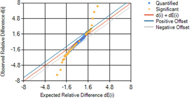
Tusher plot²⁰ produced by Proteoform Suite showing the relative difference of each of the 491 experimental proteoforms selected for quantification plotted against the expected relative difference for that quantified proteoform. The proteoforms with relative differences that exceed the positive or negative offset are considered significant along with proteoforms that changed >4-fold in at least 2 of 3 biological replicates.

Gene Ontology (GO) Analysis

The biological functions of most proteins are annotated with GO terms in the UniProt database used in Proteoform Suite. We leveraged these GO annotations to investigate whether changes in proteoforms were occurring for certain cellular functions. This provides a useful tool for assessing these changes, but we note that recent studies show that proteoforms derived from the same gene can have diverse functions.⁴ Therefore, although not currently available, a proteoform ontology in the future might allow functional analysis sensitive to differing localizations and interactions within proteoform families.

To perform the GO analysis, we first queried the set of proteins with significant proteoform-level changes. These proteins were annotated with a total of 73 GO terms. Then, we counted the number of times each GO term was observed in this set as well as a background set of 106 proteins corresponding to all quantified proteoforms. The p-value for each GO term was calculated using a hypergeometric test, and then the Benjamini–Yekutieli correction²¹ was applied to adjust for multiple testing under the dependency of the hierarchical ontology structure (Table S11). Analyzing the GO terms associated with proteoforms that changed significantly in salt stress response showed 5 GO terms were significantly overrepresented (p < 0.05): (1) “Cellular Component: nuclear nucleosome”, (2) “Molecular Function: DNA binding”, (3) “Biological Process: chromatin assembly or disassembly”, (4) “Cellular Component: replication fork protection complex”, and (5) “Molecular Function: protein heterodimerization activity”. These are each associated with the 6 histone protein entries that were observed to have significant proteoform level changes (with UniProt accessions P02293, P02294, P02309, P04911, P04912, and P61830). A second analysis using a background set of the 1742 proteins detected below 1% FDR in a bottom-up analysis (see in section 3.2 of the Supporting Information) of normal and salt-stressed yeast showed 5 additional GO terms that were significantly overrepresented (p < 0.05): (6) “Cellular Component: cytosolic large ribosomal subunit”, (7) “Biological Process: translation”, (8) “Biological Process: cytoplasmic translation”, (9) “Biological Process: sexual sporulation resulting in formation of a cellular spore”, and (10) “Biological Process: transfer RNA gene-mediated silencing”. Each GO term and corresponding p-value for this second analysis are presented in Table S12.

Visualizing Proteoform Families

The results from proteoform identification, quantification, and assembly into families are best utilized by visualizing the interconnections and changes between related proteoforms. Proteoform Suite outputs scripts that can be run by the program Cytoscape^10,11 (version 3.5 with the “enhanced-Graphics” application version 1.1.1) to produce networks of proteoform families where the individual proteoforms are represented as nodes (circles) and their connections to each other are represented as edges (lines). These scripts automatically format the families to indicate (1) the total intensity for each proteoform (size of circle), (2) the relative quantification between two conditions (pie chart), and (3) proteoforms that changed significantly between conditions (annulus around pie chart). Cytoscape session files containing full networks for all proteoform families, families with significant changes, and each of the significant GO terms can be found in the Supporting Information.

RESULTS

We collected and analyzed intact proteoform MS data for Saccharomyces cerevisiae (yeast) cultured in normal and salt-stress conditions. Proteoform Suite found 2043 unique proteoforms in this data set. Connecting proteoforms by mass differences representing known PTMs and amino acid losses (Figure 1B), or sets of these modifications, yielded 298 proteoform families containing 1110 proteoforms (Figure 7A). The remainder were not associated with other proteoforms or UniProt accession numbers; these 933 proteoforms (with 18% of all proteoform observations and 23% of all assigned quantitative components) may be identified in the future with improved databases or additional PTM identifications. Proteoform families comprise 82% of the 37,431 NeuCode pairs that represent experimental proteoform observations and 77% of the 77,341 components from the quantitative experiment that were assigned to experimental proteoforms. A total of 146 families are linked to a single gene each (520 proteoforms with 44% of all proteoform observations and 40% of all assigned quantitative components); 13 families have some ambiguity in identification in that they were associated with two or more genes (207 proteoforms with 22% of all proteoform observations and 23% of all assigned quantitative components), and the remaining 139 families are currently unidentified (383 proteoforms with 16% of all proteoform observations and 14% of all assigned quantitative components).

Figure 7.

(A) Proteoform Suite revealed 298 proteoform families containing over 1,100 proteoforms. Each identified proteoform is shown as a blue circle whose size is proportional to its integrated intensity. For simplicity, the relative quantification between normal and salt-stressed yeast is not shown (A) but is shown in the expanded view (B). (B) SBH1 proteoform family. We identified and quantified proteoforms for normal (blue) and salt-stressed yeast (yellow) and observed acetylation and phosphorylation on Sbh1 that have been suggested to have opposite regulatory effects, repressing and inducing import into the ER, respectively.²⁹ The acetylphospho form highlighted with an orange annulus changed significantly between the conditions with a > 4-fold increase in all replicates of salt stress in this case. Proteoforms in gray did not meet the requirements for quantification (i.e., the proteoform was not observed in all 3 biological replicates of at least one condition).

The structure of identified and ambiguous proteoform families can be used to identify individual experimental proteoforms, as described in the Methods section. This approach was used to identify 638 experimental proteoforms with a 4.3% false discovery rate (listed in Table S1 and comprising 62% of all proteoform observations and 60% of all assigned quantitative components). These experimental proteoforms correspond to 437 proteoforms when disregarding adducts. This is comparable to previous global studies of yeast proteoforms,⁵ and we provide additional depth to these identifications by quantifying and visualizing biological changes. Many of the identified proteoform families captured known protein variation. For example, we identified several histone proteoforms with variable numbers of acetyl groups,²² a hypusinated form of translation factor Hyp2,²³ and methylation of ribosomal proteins.²⁴

We quantified proteoform abundance changes between two conditions, normal and stressed yeast, representing the first report using an isotopic labeling strategy for combined identification and quantification of intact proteoforms. Rhoads and colleagues previously demonstrated potential of the neutron encoding (NeuCode) labeling strategy for accurate quantification of intact proteins by showing reproducible intensity changes;²⁵ this study builds upon that work by performing both global identification and quantification of thousands of proteoforms to reveal biologically relevant changes. To quantify proteoforms, we first grew the lysine auxotrophic yeast strain BY4742 in media that included light (normal growth) or heavy (salt stress) neutron-encoded (NeuCode) lysine²⁶ and then analyzed a 1:1 mixture of normal and stressed yeast lysates (Figure 1C). The light and heavy NeuCode lysines differ in mass by 0.036 Da per lysine, separating the isotopic distributions of the light- and heavy-labeled proteoforms and thereby allowing us to compare intensities of yeast proteoforms between the two conditions. Relative quantification of proteoforms between normal and salt-stress sample conditions showed 64 proteoforms exhibiting significant changes, 29 of which were identified (Table S2). Changes were considered significant if they either (a) passed permutation tests or (b) exhibited differences of 4-fold or greater for 2 of the 3 biological replicates. Built-in GO analysis of these proteoforms revealed changes in chromatin-associated proteins and machinery involved in translation (see Methods section). Proteoform Suite provides a rich view of relationships and changes in proteoforms and their families, affording an unprecedented new perspective upon global proteoform response to perturbations.

Stressed cells exhibited specific changes in histone acetylation patterns and several reproducible changes in ribosome methylation, acetylation, and oxidation that may affect translational fidelity.²⁷ We observed significant salt stress effects for proteoforms involved in the Sec61 complex, which is responsible for cotranslational import into the endoplasmic reticulum (ER). Proteoforms derived from the SBH1 gene form a subunit of the Sec61 complex,²⁸ and their family is shown in Figure 7B. Sbh1 shows prominent changes in acetylation and phosphorylation. N-acetylation of Sbh1 is thought to interfere with ER import, whereas phosphorylation may enhance import into the ER.²⁹ The proteoform family plot for SBH1 provides a striking visualization of the complexity of the different proteoforms associated with these genes and their changes in response to salt stress. Proteoform Suite facilitates the rapid generation of such plots by writing scripts for the network visualization software Cytoscape^10,11 that can be loaded in seconds, providing valuable insight into the biological changes that are manifested in proteoform families. Several other proteoform families showed significant alterations in relative abundances, and these are shown in more detail in the Supporting Information.

CONCLUSIONS

We have presented Proteoform Suite, a new open-source software tool for the identification of proteoforms and the generation and visualization of proteoform families and their changes in response to perturbations. Visualizing proteoform families provides a simple way to represent complex and related measurements in a readily interpretable form. We illustrated this in the present work by showing changes in the SBH1 proteoform family of known biological importance. The same approach could also be applied to visualize more complex proteoform families with challenging and expansive variation, such as the large proteoform groups recently described for each of four alternative splicing variations of mouse myelin basic protein.³⁰

The simplicity of identifying proteoforms from accurate intact mass measurements without fragmentation is potentially useful as a standalone tool and also as a way to possibly expand conventional top-down proteoform identifications. Although the work presented here took advantage of NeuCode tagging to provide lysine counts, we hope to eliminate the need for such tagging and extend the analysis to unlabeled proteoform samples. It is known that many more proteoform masses are observed in top-down analyses than are fragmented and identified.³¹ Extending the strategy presented here to utilize unlabeled proteoform data may be possible with highly accurate proteoform mass measurements, and that would allow both the identification of some proteoform families that were completely undetected in top-down analyses as well as the identification of previously unidentified families by leveraging top-down identifications.³² Proteoforms that are confidently identified in this way could then be quantified for normal and perturbed conditions using the code and methods already implemented in Proteoform Suite. Overall, the capability of Proteoform Suite to visualize proteoform families and their changes in response to stimuli provides an important new window into the proteomic complexity of biological systems.

ABBREVIATIONS

PTM

post-translational modification

GO

gene ontology

NeuCode

neutron encoding

OD₆₀₀

optical density at 600 nm

PBS

phosphate-buffered saline

DTT

dithiothreitol

RT

room temperature

G-PTM-D

global post-translational modification discovery

FDR

false discovery rate

Exp-Exp relation/EE relation

experimental-experimental proteoform relation

Exp-Theo/ET relation

experimental-theoretical proteoform relation

Supporting Information

The Supporting Information is available free of charge on the ACS Publications website at DOI: 10.1021/acs.jproteome.7b00685.

Section 1, Additional details on yeast proteoform families; section 1.1, Cytoscape diagrams; section 1.1.1, Identification results; section 1.1.2, Quantification results; Figure S1, Color scheme used for quantitative proteoform families; section 1.1.3, Decoy proteoform communities; section 1.2, Proteoform families with significant changes in salt stress response; Figure S2, SBH1 proteoform family with a significant change in the acetylphospho proteoform; Figure S3, NHP6A proteoform family with a significant decrease in C-terminal clipping in response to salt stress; Figure S4, NOP10 proteoform family with a significant decrease in the proteoform with methionine retention in response to salt stress; Figure S5, RTC3 proteoform family with a significant increase of the acetylated proteoform in response to salt stress; Figure S6, ZEO1 proteoform family with significant increases in a couple acetylated proteoforms or perhaps an overall increase in the abundance of the protein; section 1.3, Histone proteoform families with significant changes in yeast salt-stress response; Figure S7, HTA2 proteoform family with a significant change in the triply acetylated proteoform in response to salt stress; Figure S8, HTB1 proteoform family with a significant decrease in the unmodified proteoform; Figure S9, HTB2 proteoform family with a significant increase in the highly acetylated form and significant decreases for the monoacetylated form, both in response to salt stress; Figure S10, HHT1 proteoform family with a significant decrease in the abundance of methylated proteoforms in response to stress; Figure S11, HHF1 proteoform family with a significant decrease in the abundance of the diacetylated proteoform in response to salt stress; section 1.4, Ribosomal proteoform families with significant changes in yeast salt-stress response; Figure S12, RPS23B proteoform family with a significant decrease in the dioxidized proteoforms in response to stress; Figure S13, Ambiguous family containing RPS26A and RPS26B proteoform families; Figure S14, RPL9A proteoform family with a significant decrease in the abundance of the proteoform with retained N-terminal methionine in response to salt stress; Figure S15, RPL13B proteoform family with a significant decrease in the dimethylated proteoform in response to stress; Figure S16, RPL14A proteoform family with a significant decrease in the acetylated proteoform with one +98 Da acetone adduct;³³ Figure S17, RPL25 proteoform family with a significant decrease in the proteoform missing the C-terminal isoleucine and two oxidized forms; Figure S18, RPL29 proteoform family with a significant increase in the diacetyl form and a significant decrease in the singly oxidized form in response to salt stress; Figure S19, RPL32 proteoform family with a significant decrease in a proteoform with deamidation in response to salt stress; Figure S20, RPL35B proteoform family with a significant decrease in the abundance of a proteoform with a cleaved alanine; Figure S21, RPL39 proteoform family containing many adducts; Figure S22, RPL41B proteoform family with a significant decrease in a proteoform with a retained N-terminal methionine; Figure S23, RPL42A proteoform family with a significant decrease in the proteoform adorned with two methyl groups and one acetyl group that is also missing the N-terminal valine; section 2, Quantification validation; Figure S24, Histograms of intensity ratios for individual NeuCode pairs and for quantified proteoforms are similar, matching the expected 2:1 ratio for this experiment; Figure S25, Quantified proteoforms with an expected 2:1 intensity ratio (dotted line) have outliers with high intensity ratios that lie predominantly at lower abundances; section 3, Supporting methods; section 3.1, Protein database annotation using G-PTM-D strategy; section 3.2, Bottom-up proteomics for G-PTM-D strategy; section 3.2.1, Cell culture and lysate preparation; section 3.2.2, TCA precipitation; section 3.2.3, eFASP procedure; section 3.2.4, C18 solid-phase extraction; section 3.2.5, HPLC-ESI-MS/MS analyses; section 3.3, Removing missed monoisotopic masses and charge state harmonic errors; section 3.4, FDRs for mass difference peaks; section 3.5, Making permutations and tusher plots for permutation analysis; Table S10, Balanced permutations used in the original SAM analysis (PDF) Table S1, Identified experimental proteoforms; Table S2, Quantification results; Table S3, Raw NeuCode pairs; Table S4, Experimental proteoforms; Table S5, Theoretical proteoform database; Table S6, Exp-Theo peak mass differences; Table S7, Exp-Exp peak mass differences; Table S8, Proteoform families and orphans; Table S9, Quantification method validation using known 2:1 mixture; Table S10, Balanced permutations used in the original SAM analysis (located on page S-39 of the Supporting Information pdf); Table S11, GO analysis results: quantified proteoform background; Table S12, GO analysis results: bottom-up detected background (XLSX)

References

- 1.Smith LM, Kelleher NL. Proteoform: a single term describing protein complexity. Nat Methods. 2013;10:186–187. doi: 10.1038/nmeth.2369. [DOI] [PMC free article] [PubMed] [Google Scholar]
- 2.Whitmarsh AJ, Davis RJ. Multisite phosphorylation by MAPK. Science. 2016;354:179–180. doi: 10.1126/science.aai9381. [DOI] [PubMed] [Google Scholar]
- 3.Jenuwein T, Allis CD. Translating the histone code. Science. 2001;293:1074–80. doi: 10.1126/science.1063127. [DOI] [PubMed] [Google Scholar]
- 4.Yang X, Coulombe-Huntington J, Kang S, Sheynkman GM, Hao T, Richardson A, Sun S, Yang F, Shen YA, Murray RR, Spirohn K, Begg BE, Duran-Frigola M, MacWilliams A, Pevzner SJ, Zhong Q, Trigg SA, Tam S, Ghamsari L, Sahni N, Yi S, Rodriguez MD, Balcha D, Tan G, Costanzo M, Andrews B, Boone C, Zhou XJ, Salehi-Ashtiani K, Charloteaux B, Chen AA, Calderwood MA, Aloy P, Roth FP, Hill DE, Iakoucheva LM, Xia Y, Vidal M. Widespread Expansion of Protein Interaction Capabilities by Alternative Splicing. Cell. 2016;164:805–817. doi: 10.1016/j.cell.2016.01.029. [DOI] [PMC free article] [PubMed] [Google Scholar]
- 5.Kellie JF, Catherman AD, Durbin KR, Tran JC, Tipton JD, Norris JL, Witkowski CE, Thomas PM, Kelleher NL. Robust Analysis of the Yeast Proteome under 50 kDa by Molecular-Mass-Based Fractionation Top-Down Mass Spectrometry. Anal Chem. 2012;84:209–215. doi: 10.1021/ac202384v. [DOI] [PMC free article] [PubMed] [Google Scholar]
- 6.Catherman AD, Durbin KR, Ahlf DR, Early BP, Fellers RT, Tran JC, Thomas PM, Kelleher NL. Large-scale Top-down Proteomics of the Human Proteome: Membrane Proteins Mitochondria Senescence. Mol Cell Proteomics. 2013;12:3465–3473. doi: 10.1074/mcp.M113.030114. [DOI] [PMC free article] [PubMed] [Google Scholar]
- 7.Catherman AD, Skinner OS, Kelleher NL. Top Down proteomics: Facts perspectives. Biochem Biophys Res Commun. 2014;445:683–693. doi: 10.1016/j.bbrc.2014.02.041. [DOI] [PMC free article] [PubMed] [Google Scholar]
- 8.Shortreed MR, Frey BL, Scalf M, Knoener RA, Cesnik AJ, Smith LM. Elucidating Proteoform Families from Proteoform Intact Mass Lysine Count Measurements. J Proteome Res. 2016;15:1213–1221. doi: 10.1021/acs.jproteome.5b01090. [DOI] [PMC free article] [PubMed] [Google Scholar]
- 9.Riley NM, Mullen C, Weisbrod CR, Sharma S, Senko MW, Zabrouskov V, Westphall MS, Syka JEP, Coon JJ. Enhanced Dissociation of Intact Proteins with High Capacity Electron Transfer Dissociation. J Am Soc Mass Spectrom. 2016;27:520–531. doi: 10.1007/s13361-015-1306-8. [DOI] [PMC free article] [PubMed] [Google Scholar]
- 10.Shannon P, Markiel A, Ozier O, Baliga NS, Wang JT, Ramage D, Amin N, Schwikowski B, Ideker T. Cytoscape: a Software Environment for Integrated Models of Biomolecular Interaction Networks. Genome Res. 2003;13:2498–504. doi: 10.1101/gr.1239303. [DOI] [PMC free article] [PubMed] [Google Scholar]
- 11.Smoot ME, Ono K, Ruscheinski J, Wang P-L, Ideker T. Cytoscape 2.8: New features for data integration network visualization. Bioinformatics. 2011;27:431–432. doi: 10.1093/bioinformatics/btq675. [DOI] [PMC free article] [PubMed] [Google Scholar]
- 12.Tran JC, Doucette AA. Gel-Eluted Liquid Fraction Entrapment Electrophoresis: An Electrophoretic Method for Broad Molecular Weight Range Proteome Separation. Anal Chem. 2008;80:1568–1573. doi: 10.1021/ac702197w. [DOI] [PubMed] [Google Scholar]
- 13.Senko MW, Beu SC, McLaffertycor FW. Determination of Monoisotopic Masses Ion Populations for Large Biomolecules from Resolved Isotopic Distributions. J Am Soc Mass Spectrom. 1995;6:229–233. doi: 10.1016/1044-0305(95)00017-8. [DOI] [PubMed] [Google Scholar]
- 14.Li Q, Shortreed MR, Wenger CD, Frey BL, Schaffer LV, Scalf M, Smith LM. Global Post-Translational Modification Discovery. J Proteome Res. 2017;16:1383–1390. doi: 10.1021/acs.jproteome.6b00034. [DOI] [PMC free article] [PubMed] [Google Scholar]
- 15.Wenger CD, Coon JJ. A Proteomics Search Algorithm Specifically Designed for High-Resolution Tandem Mass Spectra. J Proteome Res. 2013;12:1377–1386. doi: 10.1021/pr301024c. [DOI] [PMC free article] [PubMed] [Google Scholar]
- 16.Solntsev SK, Shortreed MR, Frey BL, Smith LM. Enhanced Global PTM Discovery (G-PTM-D) with MetaMorpheus. Submitted for publication. [Google Scholar]
- 17.Dai Y, Shortreed MR, Scalf M, Frey BL, Cesnik AJ, Solntsev S, Schaffer LV, Smith LM. Elucidating Escherichia coli Proteoform Families Using Intact-Mass Proteomicsa Global PTM Discovery Database. J Proteome Res. 2017;16:4156–4165. doi: 10.1021/acs.jproteome.7b00516. [DOI] [PMC free article] [PubMed] [Google Scholar]
- 18.Frottin F, Martinez A, Peynot P, Mitra S, Holz RC, Giglione C, Meinnel T. The Proteomics of N-terminal Methionine Cleavage. Mol Cell Proteomics. 2006;5:2336–2349. doi: 10.1074/mcp.M600225-MCP200. [DOI] [PubMed] [Google Scholar]
- 19.Tyanova S, Temu T, Sinitcyn P, Carlson A, Hein MY, Geiger T, Mann M, Cox J. The Perseus computational platform for comprehensive analysis of (prote)omics data. Nat Methods. 2016;13:731–740. doi: 10.1038/nmeth.3901. [DOI] [PubMed] [Google Scholar]
- 20.Tusher VG, Tibshirani R, Chu G. Significance analysis of microarrays applied to the ionizing radiation response. Proc Natl Acad Sci USA. 2001;98:5116–21. doi: 10.1073/pnas.091062498. [DOI] [PMC free article] [PubMed] [Google Scholar]
- 21.Benjamini Y, Yekutieli D. The control of the false discovery rate in multiple testing under depencency. Ann Stat. 2001;29:1165–1188. [Google Scholar]
- 22.Krebs JE. Moving marks: Dynamic histone modifications in yeast. Mol BioSyst. 2007;3:590–597. doi: 10.1039/b703923a. [DOI] [PubMed] [Google Scholar]
- 23.Saini P, Eyler DE, Green R, Dever TE. Hypusine-containing protein eIF5A promotes translation elongation. Nature. 2009;459:118–121. doi: 10.1038/nature08034. [DOI] [PMC free article] [PubMed] [Google Scholar]
- 24.Polevoda B, Sherman F. Methylation of proteins involved in translation. Mol Microbiol. 2007;65:590–606. doi: 10.1111/j.1365-2958.2007.05831.x. [DOI] [PubMed] [Google Scholar]
- 25.Rhoads TW, Rose CM, Bailey DJ, Riley NM, Molden RC, Nestler AJ, Merrill AE, Smith LM, Hebert AS, Westphall MS, Pagliarini DJ, Garcia BA, Coon JJ. Neutron-encoded mass signatures for quantitative top-down proteomics. Anal Chem. 2014;86:2314–2319. doi: 10.1021/ac403579s. [DOI] [PMC free article] [PubMed] [Google Scholar]
- 26.Hebert AS, Merrill AE, Bailey DJ, Still AJ, Westphall MS, Strieter ER, Pagliarini DJ, Coon JJ. Neutron-encoded mass signatures for multiplexed proteome quantification. Nat Methods. 2013;10:332–334. doi: 10.1038/nmeth.2378. [DOI] [PMC free article] [PubMed] [Google Scholar]
- 27.Sauert M, Temmel H, Moll I. Heterogeneity of the translational machinery: Variations on a common theme. Biochimie. 2015;114:39–47. doi: 10.1016/j.biochi.2014.12.011. [DOI] [PMC free article] [PubMed] [Google Scholar]
- 28.Osborne AR, Rapoport TA, van den Berg B. Protein Translocation By the Sec61/Secy Channel. Annu Rev Cell Dev Biol. 2005;21:529–550. doi: 10.1146/annurev.cellbio.21.012704.133214. [DOI] [PubMed] [Google Scholar]
- 29.Soromani C, Zeng N, Hollemeyer K, Heinzle E, Klein M-C, Tretter T, Seaman MNJ, Römisch K. N-acetylation phosphorylation of Sec complex subunits in the ER membrane. BMC Cell Biol. 2012;13:34. doi: 10.1186/1471-2121-13-34. [DOI] [PMC free article] [PubMed] [Google Scholar]
- 30.Plymire DA, Wing CE, Robinson DE, Patrie S. Continuous elution proteoform identification of myelin basic protein by superficially porous reversed-phase liquid chromatography Fourier transform mass spectrometry. Anal Chem. 2017;89:12030. doi: 10.1021/acs.analchem.7b02426. [DOI] [PMC free article] [PubMed] [Google Scholar]
- 31.Zhao Y, Sun L, Zhu G, Dovichi NJ. Coupling Capillary Zone Electrophoresis to a Q Exactive HF Mass Spectrometer for Top-down Proteomics: 580 Proteoform Identifications from Yeast. J Proteome Res. 2016;15:3679–3685. doi: 10.1021/acs.jproteome.6b00493. [DOI] [PMC free article] [PubMed] [Google Scholar]
- 32.Schaffer LV, Shortreed MR, Cesnik AJ, Frey BL, Solntsev SK, Scalf M, Smith LM. Expanding Proteoform Identifications in Top-Down Proteomic Analyses by Constructing Proteoform Families. Anal Chem. 2017 doi: 10.1021/acs.analchem.7b04221. Just accepted. [DOI] [PMC free article] [PubMed] [Google Scholar]
- 33.Güray MZ, Zheng S, Doucette AA. Mass Spectrometry of Intact Proteins Reveals + 98 u Chemical Artifacts Following Precipitation in Acetone. J Proteome Res. 2017;16:889–897. doi: 10.1021/acs.jproteome.6b00841. [DOI] [PubMed] [Google Scholar]
Associated Data
This section collects any data citations, data availability statements, or supplementary materials included in this article.