Individual Survival Curves Comparing Subjective and Observed Mortality Risks

Abstract

We compare individual survival curves constructed from objective (actual mortality) and elicited subjective information (probability of survival to a given target age). We develop a methodology to estimate jointly subjective and objective individual survival curves accounting for rounding on subjective reports of perceived survival. We make use of the long follow-up period in the Health and Retirement Study and the high quality of mortality data to estimate individual survival curves which feature both observed and unobserved heterogeneity. This allows us to compare objective and subjective estimates of remaining life expectancy for various groups and compare welfare effects of objective and subjective mortality risk using the life-cycle model of consumption. We find that subjective and objective hazards are not the same. The median welfare loss from misperceptions of mortality risk when annuities are not available is 7% of current wealth at age 65 while more than 25% of respondents have losses larger than 60% of wealth. When annuities are available and exogenously given, the welfare loss is substantially lower.

1 Introduction

Mortality expectations play a key role in economic models of saving behavior (Yaari, 1965; Hamermesh, 1985; Hurd, 1989). Examining these models with data requires modelling of mortality expectations. Earlier work assumed individuals expected mortality to follow population mortality risk. Most studies use aggregate mortality found in life tables (e.g. Hubbard et al., 1995; Scholz et al., 2006). Recognizing that mortality risk is heterogeneous across individuals, recent work has used actual mortality risk conditional on observable characteristics (e.g. De Nardi et al., 2011). Indeed, rich datasets such as the Health and Retirement Study accurately record the mortality experience of respondents over a period of more than 20 years. Hence, analysis of mortality can be conditioned on known socio-economic covariates. Despite being an improvement, using observed (or objective) mortality in models of economic behavior, whether from life tables or from panel data, requires that individuals correctly assess their mortality risk. Groups may vary in their ability to predict their own mortality risk (Lichtenstein et al., 1978; Khwaja et al., 2006). Since longevity risk is paramount for retirement preparation, misperceptions of mortality risk could have far reaching implications for well-being in retirement.

The Health and Retirement Study has pioneered the collection of perceived, or subjective, mortality risk. It asks respondents to provide a point estimate of their probability of surviving to a target age. Several studies show that subjective survival probabilities aggregate well to life-table probabilities and that they covary with various characteristics in expected ways (Hurd and McGarry, 1995). Also, they are predictive of actual mortality risk, even when conditioning on a rich set of socio-economic and demographic variables (Hurd and McGarry, 2002). Several studies analyze the predictive power of subjective report of mortality risk for a number of economic decisions (Hurd et al., 2004; Dominitz and Manski, 2007; Salm, 2010). Yet subjective mortality risk has not been used extensively in life-cycle models of saving behavior.

There are two important impediments to using these data in economic models. First, a single point estimate of a subjective survival probability to a target age cannot be directly transformed into subjective survival curves to compute expected utility. One could compare the predicted life-table survival probability to the same target age to apply a proportional shift to the life-table mortality profile. Gan et al. (2005) adopt a sophisticated variant of this strategy. The main limitation of this approach is that the life-table may not be an appropriate benchmark due to cohort and selection effets. Another limitation is that some respondents do not answer subjective risk questions. Such respondents typically have greater mortality risk than others.

Second, subjective reports of survival probabilities appear to be rounded. This introduces additional complexity as reports of a subjective probability of zero or one yields impractical survival curves. There is also evidence that reports of focal points, such as 0.5, are quite frequent and may reflect epistemic uncertainty (de Bruin et al., 2000).

In this paper, we use 16 years of actual mortality experience for Health and Retirement Study respondents who also answered mortality-risk expectation questions. We estimate jointly objective and subjective mortality-risk models, which allows direct testing of parametric restrictions imposed by the assumption that respondents correctly perceive their actual mortality risk. We also account for rounding in reports of subjective mortality risk. Once rounding is filtered we recover individual subjective survival curves which vary both due to observable socio-economic characteristics and unobserved heterogeneity in subjective reports. Finally, we use the standard life-cycle model to show how consumption paths derived from subjective survival expectations may differ from those using objective (or rational) survival expectations.

We report a number of novel findings. The life-table appears not to be the correct benchmark for validating expectations in surveys such as the HRS, in particular for females. Using actual mortality in HRS, we reject that objective and subjective mortality hazards equations are the same. Respondents appear to overestimate the benefits of education in terms of survival while they correctly perceive the rate of the decline in survival with age. Rounding is widespread, 33.7% round to the nearest multiple of 50 while only 1.7% report precise answers (no rounding). Overall, respondents overestimate their remaining life expectancy (1.5 years for males and 0.8 years for females). While at the median smokers and non-smokers correctly perceive their remaining life expectancy, distributions are characterized by heavy tails such that on average smokers are too optimistic. Finally, we compute the welfare loss of misperceiving mortality risk in a standard life-cycle model of consumption. At the median, the welfare loss is 7% at age 65 which is large. More than 25% of respondents have welfare losses larger than 60% of their wealth.

The paper is structured as follows. In Section 2, we describe the data and discuss the questions used to elicit subjective survival probabilities. In Section 3, we present the models of subjective survival. In Section 4, we present the estimation results. Section 5 presents an application to consumption trajectories in retirement. Section 6 concludes.

2 Data

We use data from the Health and Retirement Study (HRS) relying on nine waves from 1992 to 2008. The sample includes respondents aged 50 and older, and their spouses. Death is recorded in exit interviews and confirmed with matches to the National Death Index (NDI). Respondents for whom the vital status is unknown are also matched to the NDI to collect death information of deceased respondents. We use covariates measured in the current wave to predict mortality by the following interview.

2.1 Observed Survival

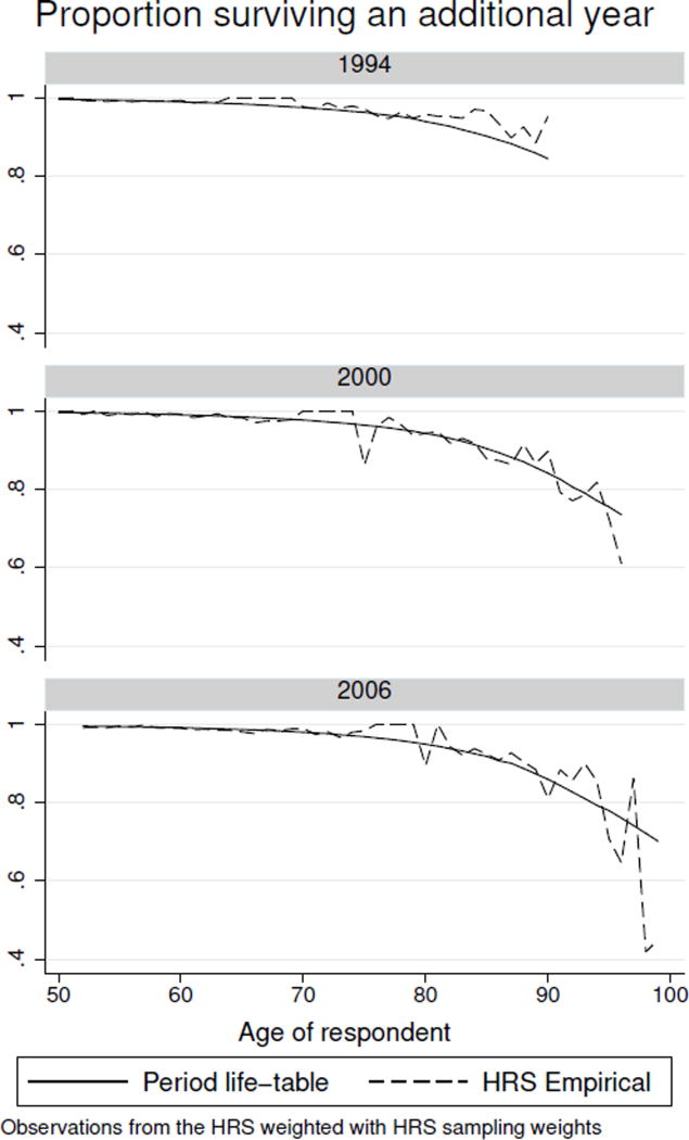
Figure 1 compares between-period life-table and one-year survival rates from the survey in three waves of the HRS. For this, we use all respondents answering in that wave as well as year-of-death from the HRS/NDI information to compute the fraction who are known to have survived one year. These data from the HRS use respondent-level weights for each of these three years. We obtain period life tables from the Human Mortality Database (www.mortality.org).

Figure 1.

Comparison of the survival rate over one year at various ages between the HRS respondents in 1994, 2000, and 2006 with the period life-table for these years.

For all three years, the HRS survival and period life-table survival rates match well prior to age 75. HRS survival is somewhat higher at older ages in 1994, but this difference vanishes by 2006. This difference is likely due to the sampling frame the HRS used. The HRS samples the non-institutionalized population for each entering cohort entering the study. The non-institutionalized population has more favorable survival prospects than the overall population. The gap vanishes as the study progresses because HRS follows respondents who enter nursing homes. Hence, if the objective is to compare actual and expected survival, it is therefore important to use the actual mortality experience of those answering the expectations questions.

2.2 Subjective Survival

The HRS elicits subjective survival expectations through the following question:

[Using any] number from 0 to 100 where “0” means that you think there is absolutely no chance and “100” means that you think the event is absolutely sure to happen… What do you think are chances that: You will live to at least A?

where A is a target age that varies for each respondent. Respondents 65 or younger were asked to report a probability of survival to age 75. Respondents older than 65 were asked about survival to another target age. This target age was determined as an age 11 to 15 years in the future that is also a multiple of 5 (e.g. 90 for an individual aged 78). Our analysis includes 18,791 respondents who answered the probability questions, were observed at least once alive, and provided information on the covariates included in the analysis. When using the full sample, the number of observations (i.e. respondent-wave) is 80,298. Because we compare actual mortality of individuals who respond to the subjective probability question, we do not need to account for the selective nature of non-response to this question.

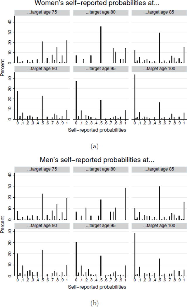
The self-reported probabilities are subject to rounding and focal answers (0, 0.5 and 1). Figures 2 (a) and (b) present histograms showing the distribution of the elicited subjective probabilities for the 6 target ages separately for females and males. There is substantial heterogeneity in the reported probabilities but significant heaping at the multiples of 50%-points (0, 50 and 100%). The proportion of such answers is rather stable for each target age. Answers of 0% and 100% are particularly problematic given that they imply degenerate hazard rates (infinity or 0). We also find evidence of rounding at multiples of 25, 10, and 5, and also find very precise answers reported with a 1%-precision. Our empirical strategy allows for the possibility of rounded answers.

Figure 2.

Histograms of the self-reported probabilities of survival to various target ages for women (a) and men (b). The target age depends on the respondent’s age, hence respondents in the same sub-figures are close in age.

2.3 Observed Characteristics

We use several dummy variables (taking a value of 1) throughout our analyses. These are for respondents who are male, black, Hispanic, whose highest educational attainment is a high-school diploma, whose highest educational attainment is a college degree, and who were smoker at one point in their life. The selected covariates are known to influence mortality and are typically constant over time for a given respondent. We include cohort dummies to control for variations in survival probabilities among older respondents that would not be captured by observable characteristics. We only consider characteristics which can be assumed not to vary with age because we seek to predict survival curves that covary with observable characteristics.

3 Econometric Model

We develop an econometric model for reports of subjective survival expectations which allows us to compare subjective and objective mortality hazards. Since both hazards are parametrized in similar ways, we can also construct subjective and objective survival curves. The model accounts for rounding in subjective survival probabilities. The model consists of three components:

1. the objective hazard to predict survival among a population of respondents with given characteristics;

2. the subjective hazard perceived by respondents with given characteristics, and for whom the objective hazard is a special case;

3. the reporting model, accounting for the rounding behavior of respondents.

We present in this section the main equations of the estimated model. Additional details on how we obtained these equations are available in Appendix A.

3.1 Objective hazard

Consider a respondent i at age a when reporting a probability of survival to target age t. We are interested in the probability that the age of death of the respondent, denoted T, will be greater than t. This probability is given by:

$$S_a(t|{\mathit{x}}_{\mathit{i}},{\nu }_i)=\text{exp }(-{\int }_a^t{\nu }_i\lambda (\tau |{\mathit{x}}_{\mathit{i}})d\tau )$$ (1)

where the objective hazard of respondents i can be separated in two parts. First, λ(t|x_i) is the homogenous baseline hazard, common to respondents with observed characteristics x_i. Then, ν_i is a frailty term added to capture unobserved heterogeneity (unobserved to analysts). An alternative representation in terms of the integrated hazard if given by:

$$S_a(t|{\mathit{x}}_{\mathit{i}},{\nu }_i)=\text{exp}(-{\nu }_i{\mathrm{\Lambda }}_a(t|{\mathit{x}}_{\mathit{i}}))$$ (2)

where Λ_a(t|x_i) is the integrated objective hazard from age a to age t.

We assume a proportional hazard where the baseline hazard takes the Gompertz form.¹ The homogenous part of the hazard at age t, for a respondent with characteristics x_i, constant over time, is given by:

$$\lambda (t|{\mathit{x}}_{\mathit{i}})=\text{exp}({\mathit{x}}_{\mathit{i}}\mathit{\zeta })\text{ exp}(\alpha t).$$ (3)

Respondents are first observed after age 50. We therefore use age 50 as our initial time at risk. The baseline integrated hazard from the initial time period (notice that we omit the subscript a in this case) is then given by:

$$\mathrm{\Lambda }(t|{\mathit{x}}_{\mathit{i}})=\frac{\text{exp}({\mathit{x}}_{\mathit{i}}\mathit{\zeta })}{\alpha }(\text{exp}(\alpha t)-1).$$ (4)

Furthermore, we assume that the individual frailty term ν follows a gamma distribution with unit expectation and a variance of $\frac{1}{\delta }$ at the initial time at risk. Under these assumptions, the survival probability from age a to age t is given by (see Section A.1 for details):

$$S_a(t|{\mathit{x}}_{\mathit{i}})={\left(\frac{\delta +\mathrm{\Lambda }(a|{\mathit{x}}_{\mathit{i}})}{\delta +\mathrm{\Lambda }(t|{\mathit{x}}_{\mathit{i}})}\right)}^{\delta }.$$ (5)

Each respondent is observed last at a given age, either the age at death or the age at the last interview for respondents still alive. We denote this age by t_i. We observe respondent i entering the survey at age a_i. Additionally, as some respondents are still alive at time t_i, we account for right censoring. The likelihood contribution of an individual i is given by:

$$L^O(\zeta ,\alpha ,\delta |{\mathit{x}}_{\mathit{i}},a_i,t_i)=\lambda {(t_i|{\mathit{x}}_{\mathit{i}})}^{d_i}{S}_a(t_i|{\mathit{x}}_{\mathit{i}})$$ (6)

where d_i is a dummy variable taking the value 1 if the respondent is deceased at time t_i.

3.2 Subjective Hazard

We use the superscript S to denote the subjective components of the model. We use the same parametric specification so as to compare objective and subjective parameters directly. Should the agents correctly perceive their mortality risk, their subjective and objective hazards would be identical. Using a similar notation for subjective probability of survival, we define:

$$S_a^S(t|{\mathit{x}}_{\mathit{i}},{\nu }_i^S)=\text{exp }(-{\int }_a^t{\nu }_i^S{\lambda }^S(\tau |{\mathit{x}}_{\mathit{i}})d\tau )=\text{exp }(-{\nu }_i^S{\mathrm{\Lambda }}_a^S(t|{\mathit{x}}_{\mathit{i}})).$$ (7)

To interpret directly differences between objective and survival hazards we reparametrize using:

$${\alpha }^S=\alpha +{\psi }_{\alpha }$$

$${\mathit{\zeta }}^S=\mathit{\zeta }+{\mathit{\psi }}_{\zeta }$$

$${\delta }^S=\delta +{\psi }_{\delta }.$$

Hence, under the null hypothesis of correctly perceived mortality risk, ψ_ζ, ψ_α, and ψ_δ are equal to 0.

3.3 Self-reports and Rounding

We assume that the self-reported survival probability p_iat is a rounded report of $S_a^S(t|{\mathit{x}}_{\mathit{i}},{\nu }_i^S)$. We use a latent-variable reporting model following Heijtan and Rubin (1990,1991) and Kleinjans and van Soest (2013). We do not know the rounding rule used by the respondents. The problem of unknown rounding is comparable to a problem of unknown mixture of distributions. Suppose that we observe a respondent answering 25% to a probability question. The answer could be the result of rounding of a subjective probability in the [12.5, 37.5) range, rounding at the nearest multiple of 25. It could also come from the [22.5, 27.5) range if a respondent rounded to the nearest multiple of 5, or even from the [24.5, 25.5) range should a respondent give a very precise answer. Based on distributional assumptions, we can estimate a model predicting the probability that respondents will use various rules in rounding and use that for maximum likelihood inference.² We consider the following rules based on what we observe from data:

1. Throw-away 50%-points reflecting epistemic uncertainty (cf. de Bruin et al., 2000). In these cases, the answer 50%-points is similar to a non-response;³

2. Rounding to a multiple of 50%-points;

3. Rounding to a multiple of 25%-points;

4. Rounding to a multiple of 10%-points;

5. Rounding to a multiple of 5%-points;

6. Precise answers rounded at 1%-points.

We treat the rounding rule as an unknown random variable R. We denote the realization of R with r, an integer from 1 to 6 according to the above list. Hence, a higher value means a more precise answer or less rounding. Each rounding rule leads to a set of admissible p_iat. This set of admissible values is denoted by Ω_r. For instance, the set of admissible answer for the 25% rounding rule is {0, 25, 50, 75, 100}. Finally, for each rounding rule, a self-reported probability of p_iat can result from rounding of values between l_r(p_iat) and u_r(p_iat).

The contribution to the subjective likelihood for this individual will be given by the probability to observe the self-reported answer of p_iat. Given the rounding process described above, this probability would be given by the following equation:

$$\begin{gathered} \text{Prob}(p_{\mathit{\text{iat}}}|{\mathit{x}}_{\mathit{i}},{\mathit{z}}_{\mathit{i}})=\sum _{r=1}^{6}1(p_{\mathit{\text{iat}}}\in {\mathrm{\Omega }}_r)\times \text{Prob}(R_i=r,|{\mathit{z}}_{\mathit{i}}) \\ \times \text{Prob}(l_r(p_{\mathit{\text{iat}}})\le S_a^S(t|{\mathit{x}}_{\mathit{i}},{\nu }_i^S)<u_r(p_{\mathit{\text{iat}}})) \end{gathered}$$ (8)

where z_i corresponds to a set of characteristics which affect the likelihood of rounding. Each element of the sum on the the right contains three parts. To illustrate their role in the model, consider the following example. Suppose that a respondent gives an answer of 65%. Two events can lead to this answers.

1. The respondent is using the 5% rouding rule and his probability lies between 62.5% and 67.5%.

2. The respondents is using the 1% rouding rule and his probability lies between 64.5% and 65.5%.

Hence, the first part will allow us to consider only the rounding rules compatible with an answer, the second will determine the probability that this rounding rule was used by a respondent, and the last one will determine the probability that the subjective expectations lies in an interval that would lead to p_iat given the rounding rule of interest.

3.3.1 Modelling the probability of a rounding rule

In order to estimate the probability of using one of these six rounding rules, we follow an approach similar to the one discussed by Kleinjans and van Soest (2013). We consider that each respondent has a “propensity to provide a precise answer”, which is represented by $r_i^{\ast }$. A higher value for this variable implies that respondents are more likely to use a precise rounding rule. To capture the propensity to round, we use an ordered response model. We assume that:

$$r_i^{\ast }={\mathit{z}}_{\mathit{i}}\mathit{\gamma }+{\epsilon }_i$$

and that a respondent uses rounding regime r if $m_{r-1}<r_i^{\ast }\le m_r$, where m₀ = −∞, m₁ = 0, and m₆ = ∞. It follows that m₂ to m₅ are parameters to be estimated. We assume that ε_i follows a standard normal distribution. We then obtain:

$$\text{Prob}(R_i=r,|{\mathit{z}}_{\mathit{i}})=\mathrm{\Phi }(m_r-{\mathit{z}}_{\mathit{i}}\mathit{\gamma })-\mathrm{\Phi }(m_{r-1}-{\mathit{z}}_{\mathit{i}}\mathit{\gamma })$$ (9)

to be substituted in Equation 8. We include two additional explanatory variables in the reporting mode, leading to two exclusion restrictions. The first one is based on the number of words that a respondent could recall in a memory exercise, in order to capture cognitive skills. The variable used is a period z-score, to correct for the varying number of words asked in total and for possible variation in the difficulty of the list in a given period. The second variable is the proportion of answers that were multiples of 50 in the other probability questions of the HRS.

3.3.2 Modelling the probability that the subjective probability lies within an interval

The last part of the reporting model requires to compute the probability that a respondent’s subjective probability lies within an admissible interval. To do so, we must determine the distribution function of this subjective probability at the respondent’s age a. Conditional on the observables, the stochastic part of the subjective probability comes from the inclusion of the frailty term ν^s. We know from Equation 2 that the subjective probability falls in an interval [l, u) if ν^s falls between $-\frac{\text{ln}(l)}{{\mathrm{\Lambda }}_a^S(t|{\mathit{x}}_{\mathit{i}})}$ and $-\frac{\text{ln}(l)}{{\mathrm{\Lambda }}_a^S(t|{\mathit{x}}_{\mathit{i}})}$. Hence, the probability that the subjective probability lies within the interval is given by:

$$\begin{gathered} \text{Pr}(l\le S^S<u|T>a,{\mathit{x}}_{\mathit{i}}) \\ =F_{\nu s}(-\frac{\text{ln}(l)}{{\mathrm{\Lambda }}_a^S(t|{\mathit{x}}_{\mathit{i}})}|T>a,{\mathit{x}}_{\mathit{i}})-F_{\nu s}(-\frac{\text{ln}(u)}{{\mathrm{\Lambda }}_a^S(t|{\mathit{x}}_{\mathit{i}})}|T>a,{\mathit{x}}_{\mathit{i}}) \end{gathered}$$ (10)

We made the assumption that the frailty term follows a Gamma distribution with unit expectation at the initial time at risk, but this is not the case anymore at age t. This is caused by the fact that the frailer individuals tend to leave the population earlier, meaning the mean and the variance of the distribution of frailty will decrease over time. However, we can show that the distribution of frailty conditional on surviving at time t is a Gamma distribution with an expected value of $\frac{\delta }{{\mathrm{\Lambda }}_a^S(t|{\mathit{x}}_{\mathit{i}})+\delta }$ and a variance of $\frac{\delta }{{({\mathrm{\Lambda }}_a^S(t|{\mathit{x}}_{\mathit{i}})+\delta )}^2}$ (see Section A.2 for details).

3.4 Likelihood

We estimate the model by maximum likelihood. We maximize the joint likelihood of observing self-reported subjective probabilities and actual mortality. The likelihood for the subjective reports is

$$L^S(\mathit{\zeta },\alpha ,\delta ,{\mathit{\psi }}_{\zeta },{\psi }_{\alpha },{\psi }_{\delta },\gamma |{\mathit{x}}_{\mathit{i}},a_i,{\mathit{z}}_{\mathit{i}})=\text{Pr}(p_{\mathit{\text{iat}}}|{\mathit{x}}_{\mathit{i}},{\mathit{z}}_{\mathit{i}})$$

which can be computed by substituting Equations 9 and 10 in Equation 8.

The complete likelihood is given by:

$$\text{ln }L=\text{ln }{L}^O+\text{ln }{L}^S.$$ (11)

Given that we estimate both objective and subjective hazards jointly, we can test whether parameters differ.⁴

3.5 Subjective Frailty and Individual Curves

Once we estimate the parameters, we can generate individual subjective survival curves for each respondents. Assuming that we knew the value of the unobserved frailty term, the survival curve would be obtained by evaluating Equation 7. Given that we do not know this term, we must use the self-reported rounded probability p_iat to obtain a distribution of ${\nu }_i^S$. In the remainder of the paper, we impute for each respondent the expected value of ${\nu }_i^S$, conditional on the answer to the self-reported survival probability, and will use this value to derive the expected survival curve. The expression for this expectation is given by

$$E({\nu }_i^S|p_{\mathit{\text{iat}}},{\mathit{x}}_{\mathit{i}},{\mathit{z}}_{\mathit{i}})=\frac{{\int }_0^{\infty }u\text{Prob}(p_{\mathit{\text{iat}}}|u,{\mathit{x}}_{\mathit{i}},{\mathit{z}}_{\mathit{i}})f_{\nu s}(u|{\mathit{x}}_{\mathit{i}},T>a)\mathrm{d}u}{\text{Prob}(p_{\mathit{\text{iat}}}|{\mathit{x}}_{\mathit{i}},{\mathit{z}}_{\mathit{i}})}.$$ (12)

We use numerical method to find the value for each respondent. Hence, the resulting survival curves account for both differences in observable and unobservable determinants of subjective mortality risk.

4 Estimation Results

4.1 Objective Survival Curves

We report estimates of objective hazard parameters in the first column of Table 1. A positive parameter implies higher mortality risk and thus lower survival probability. Mortality risk covaries in expected ways with demographic characteristics. Cohort-effect estimates suggest that mortality risk is higher for younger cohorts. This would suggest a decrease in longevity in years to come. An alternative explanation is that this is due to selection in HRS. The HRS samples from the non-institutionalized population and the entry cohort in AHEAD (70+ at entry) could well be healthier than younger cohorts who reach age 70 whether they are institutionalized or not.

Table 1.

Estimation results

	Objective modela (ζO, αO, and δO)	Subjective modelb (ψ, ψα, and ψδ)	Reporting model (γ and mr)
Male	0.272 (0.029)	−0.151 (0.031)	0.012 (0.010)
Black	0.216 (0.040)	−0.220 (0.042)	−0.101 (0.015)
Hispanic	−0.092 (0.058)	0.403 (0.062)	0.004 (0.020)
High School	−0.210 (0.033)	−0.103 (0.036)	−0.008 (0.013)
College	−0.379 (0.035)	−0.220 (0.037)	0.188 (0.013)
Ever Smoked	0.427 (0.034)	−0.245 (0.035)	0.013 (0.011)
Cohort 1900–1915	−0.537 (0.071)	0.791 (0.125)	0.274 (0.026)
Cohort 1915–1930	−0.440 (0.056)	0.253 (0.063)	0.199 (0.013)
Cohort 1930–1945	0.146 (0.098)	−0.195 (0.099)	−0.000 (0.017)
α	0.109 (0.004)	0.006 (0.004)
δ−1	0.016 (0.042)	1.080 (0.043)
Immediate word recall (z-score)			0.018 (0.007)
Prop. of 0/50/100 in other quest.			−1.288 (0.021)
Constant (ζ0, ψ0, or γ0)	−5.984 (0.077)	0.851 (0.081)	4.560 (0.245)
m2			3.629
m3			4.063
m4			5.290
m5			6.322
N	18,791	80,298
Log-likelihood		−219,686.042

Standard errors in parentheses

^aSurvival model estimated using age 50 as initial time period.

^bSubj. parameters expressed in terms of differences as in equations 5.7 to 5.9.

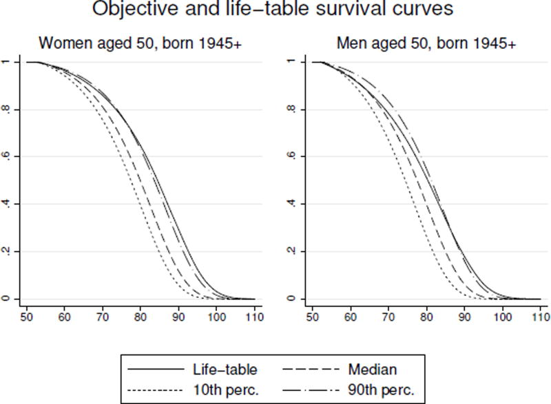
In Figure 3, we present for men and women separately the distribution of individual curves based on objective risk for the respondents born in 1945 or later and aged 50 to 53 at baseline –the youngest respondents of our sample. We report 10th, 50th (median) and 90th percentile of the curves. We also report the period life-table survival curve for the year the median respondent answered the survey (i.e., 1998). We use sample weights.

Figure 3.

Comparison of the objective and of the life-table-based survival curves. Percentiles in this figure were determined using HRS weights.

The median life-table and objective curves are close for men but differ for women. The median survival curve for women lies below the life-table survival curve. Hence, the HRS features higher mortality for women than the life-table. Hurd and McGarry (2002) report a similar finding over earlier waves.⁵ This finding highlights one of the main advantages of the approach we propose: even with a nationally representative sample like the HRS, the life-tables may not be a valid measure of within-sample survival probabilities. Deviation from the life-tables in subjective expectations may not be due to erroneous predictions of respondents.

4.2 Subjective Survival and Reporting

The second column of Table 1 contains estimated parameters for the subjective hazard ψ_ζ, ψ_α, and ψ_δ, capturing differences between the objective and subjective parameters.

We find that men, black and more educated (either with a high school or college degree), younger-cohort, and smoking respondents have higher subjective survival than objective survival. Hence, they are more optimistic than other groups. Hispanic respondents appear to have lower subjective survival rates. Hence, they are more pessimistic. The negative signs of the estimates of both education dummies also show that respondents overestimate the benefits of education for survival.

Differences between α^O and α^S are small and statistically insignificant (p-value = 0.154) which suggest that respondents do well at predicting the rate of decline in their survival probabilities. The difference in baseline risk (intercept) is larger than zero. Hence, respondents are more pessimistic at younger ages about their survival regardless of differences in characteristics.

The variance of the frailty term is much larger for subjective frailty than it was for objective frailty, implying higher perceived variation among respondents regarding mortality than we found with actual data. This is consistent with Hamermesh (1985).

A Wald test of joint significance rejects strongly the null hypothesis that all differences in parameters across hazards are zero. Hence, evidence suggest that there is little support for using objective risk in models of behaviour because respondents make decisions based on subjective survival curves which deviate substantially from objective curves.

In the last column of Table 1, we present results for the rounding model. We find that being male, Hispanic, having a high school diploma, and ever smoking are very weakly related to rounding behavior. College education and cognitive skills increase the likelihood of more percise answers. We also find that a higher proportion of focal answers in other HRS questions leads to a higher probability of coarse rounding in the self-reported survival probability, reinforcing the idea that some respondents are simply less prone to give "precise" answers. We find little support for the idea that 50%-point answers are used to avoid answering questions. In our model, the predicted probability of such behavior is practically zero for all respondents. On average, we predict that 33.7% of the respondents round to the nearest multiple of 50, while 15.8% round to a multiple of 25, 37.8% to a multiple of 10, 11.0% to a multiple of 5, and 1.7% report very precise answers.

We assess whether rounding is important by re-estimating a model where we fixed the propensity to report precise answers to one. This implies that we assume that respondents report their subjective probabilities with a 1%-point precision. The variance of the subjective frailty term in that model is about twice as large when we do not take rounding into account, increasing to a value of 2.63 with a standard error of 0.04. The variation in frailty needed to accommodate the large fraction of respondents who used 0% and 100% is quite substantial when there is no rounding. Other parameters adjust in terms of magnitude.

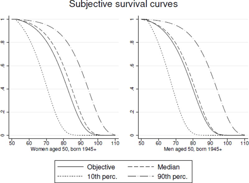
In Figure 4, we present the distribution of subjective curves. We also plot the median objective survival curve. For each respondent, we compute the expected subjective frailty term as described in Equation 12 and use those to trace survival curves.

Figure 4.

Subjective survival curves conditional on the respondents’ self-reported probabilities (expected subjective frailty used).

We observe that the median objective and subjective curves are quite close. This would imply that women are conscious of the higher-than-predicted mortality risk. We also see evidence that both men and women are slightly optimistic. There is substantial heterogeneity in subjective curves, more so than in objective curves.

4.3 Subjective Remaining Life Expectancy

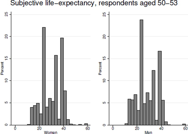
We can use subjective survival curves to compute subjective remaining life expectancy. In Figure 5, we report remaining subjective life expectancy at age 50. Estimates of average remaining objective life expectancy risk are 26.5 years for men and 29.2 years for women. The average subjective remaining life expectancy is 28.0 years for men and 30.0 years for women.

Figure 5.

Distribution of the conditional life-expectancy (in remaining years) for the respondents aged 50–53, all cohorts combined.

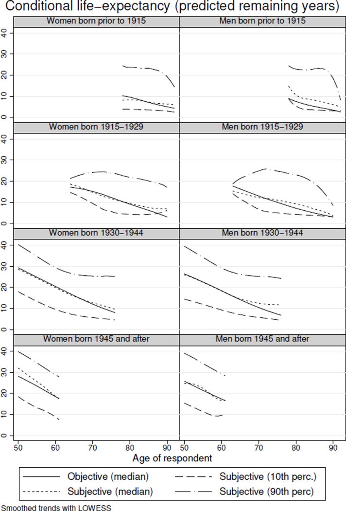
We also report the distribution of remaining life expectancy by age, gender and cohort in Figure 6 along with median objective survival prediction at each age. These profiles are smoothed in order to focus on variation induced by the model rather than sampling variation.

Figure 6.

Objective and subjective life-expectancy (in remaining years) at various ages, by gender and cohort

Median subjective and median objective predictions are very similar for all groups. As expected from Figure 4, median respondents have subjective expectations that are quite close to the objective ones. There is considerable dispersion in the subjective estimates.

4.4 Education

Differences in life expectancy may be important for understanding lack of preparation for retirement. Scholz et al. (2006) find that roughly 20% of households, particularly those with less education in the HRS appear to be saving too little relative to savings predicted from a model which uses lifetable mortality risk. This would also imply that 80% may be saving too much for retirement. Savings behavior has important welfare implications.

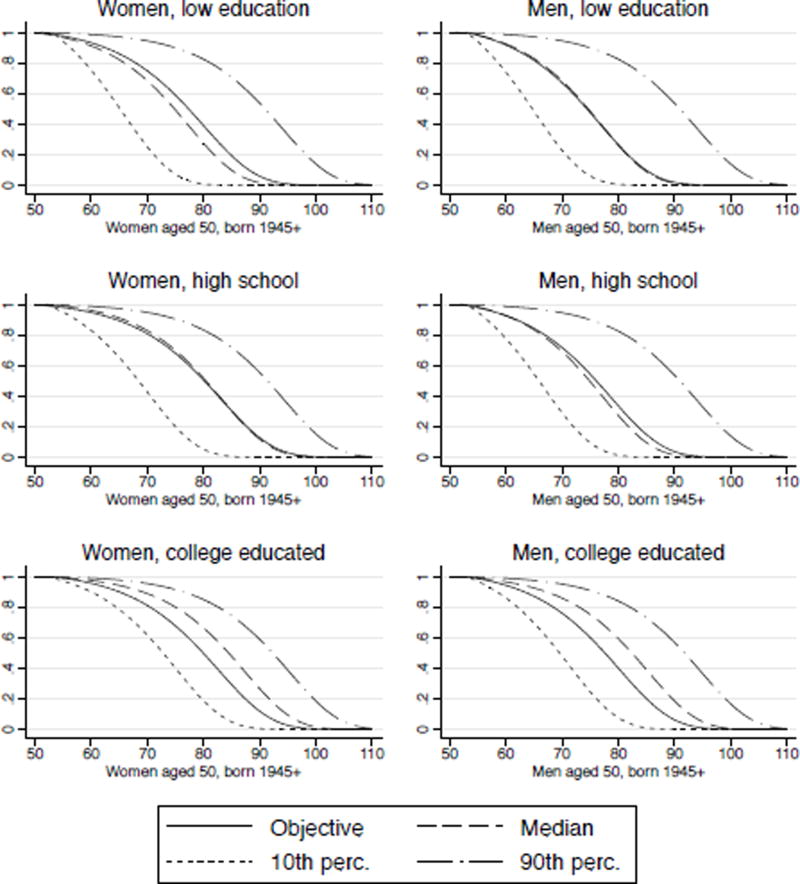
Figure 7 compares survival curves for three education groups of men and women. For men, those with low education tend to correctly perceive their mortality risk at the median. Women with low education are slightly pessimistic about their survival prospects. For both men and women of low education, there is considerable heterogeneity in survival expectations, more so than for more educated groups (high school, college). There tends to be less variance in survival curves for college-educated men. At the median, such men tend to be optimistic about their survival prospects. Given that they overestimate the number of years for which they need to finance retirement consumption, they may be saving more than necessary.

Figure 7.

Subjective survival curves conditional on the respondents’ self-reported probabilities (expected subjective frailty used) presented separately by level of education.

4.5 Smoking

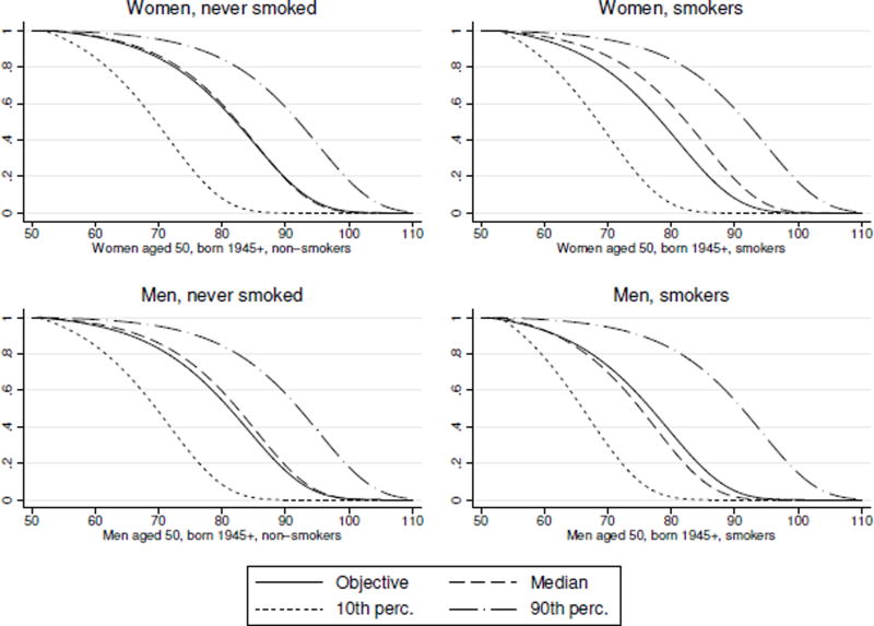
The accuracy of the expectations of smokers was previously studied by Khwaja et al. (2007) who found, using the HRS and relying on a similar comparison between subjective and objective probability of survival, that smokers tend to be optimistic concerning their own survival probabilities. Here we can compare entire survival curves for both smokers and non-smokers. In Figure 8, we present subjective survival curves of smokers and non-smokers for respondents aged 50 to 53 from the 1945 cohort. We also report the objective survival curve of the median respondent.

Figure 8.

Subjective survival curves conditional on the respondents’ self-reported probabilities (expected subjective frailty used) presented separately for smokers and non-smokers.

The median smokers and non-smokers appear to correctly perceive mortality risk. Yet this hides considerable heterogeneity. If we take the ratio of subjective to objective remaining life expectancy, we see non-smokers on average perceive correctly their mortality risk, with an average ratio of 0.99 for women and 1.03 for men. However, smokers tend to be too optimistic with an average ratio of 1.10 in subjective to objective life expectancy for both women and men. Hence, individual survival curves allow us to assess not only differences in averages but also quantify the distribution of mortality risk across individuals.

5 Consumption and Mortality Risk

The differences shown above suggest that consumers may make different decisions when using subjective rather than objective risk. For example, suppose a 65 year old believes his remaining life expectancy is 20 years but that in fact his objective remaining life expectancy is 15 years. He will plan to have enough savings to finance five additional years of consumption. Exactly how this may impact his savings and consumption will depend on his preferences. The standard life-cycle model with mortality risk dates back to Yaari (1962). In what follows, we show using a simple model of how the consumption path derived from subjective survival curves may differ from those using objective risk and compute a welfare measure that captures the loss in well-being from using incorrect beliefs.

Denote the subjective survival probability $s_t^S$, and the objective $s_t^O$. Define $c_t^S,c_t^O$ to be consumption at age t derived using subjective and objective probabilities respectively. Let r be the interest rate with R = (1 + r) and W be wealth at t = 0 which we will assume to be age 65. We will assume preferences are constant relative risk aversion, $u(c)=\frac{c^{1-\sigma }}{1-\sigma }$ and the consumer discounts the future with a factor β. Expected discounted utility conditional on using particular survival probabilities j is given by

$$U(c^j,s^j)=\sum _{t=0}^T{\beta }^t{s}_j^{j}u(c^j)$$ (13)

for j = S, O.

Given that s^j > 0 for all t and that marginal utility is negative and infinite at c_t = 0, optimal wealth is always positive at t + 1 (the consumer will not want to run the risk of surviving with no resources). Using that, the budget constraint is given by

$$W=\sum _{t=0}^T{R}^{-t}{c}_t^j$$ (14)

This simply says that wealth at t = 0 is equal to the present value of the consumption flow. We abstract from annuity income for this illustration which would make the problem more complicated (Hurd, 1989).

From the first-order condition to the maximization of U, we know that

$$\frac{c_{t+1}^j}{c_t^j}={\left(\frac{s_{t+1}^j}{s_t^j}R\beta \right)}^{\frac{1}{\sigma }}$$ (15)

and therefore

$$c_t^j=c_0^j{(s_t^j{(R\beta )}^t)}^{\frac{1}{\sigma }}=c_0^j{g}_t(s_t^j)$$ (16)

which in turn implies that the path of consumption over time can be written as a function of W:

$$c_t^j(W)=\frac{g_t(s_t^j)}{{\sum }_{t=0}^T{R}^{-t}{g}_t(s_t^j)}W.$$ (17)

Hence, the optimal consumption path given s^j and W is $c^j(W)={\{c_t^j(W)\}}_{t=0}^T$. If R = β consumption still declines with age due to mortality risk (Hurd, 1989).

Given that consumption is proportional to wealth, we will normalize accumulated wealth to one at age 65. Following Scholz et al. (2006), we will assume σ = 3, β = 0.96 and R = 1/β so as to focus on the role of mortality risk. Choosing a lower value for σ would make consumption more sensitive to mortality risk.

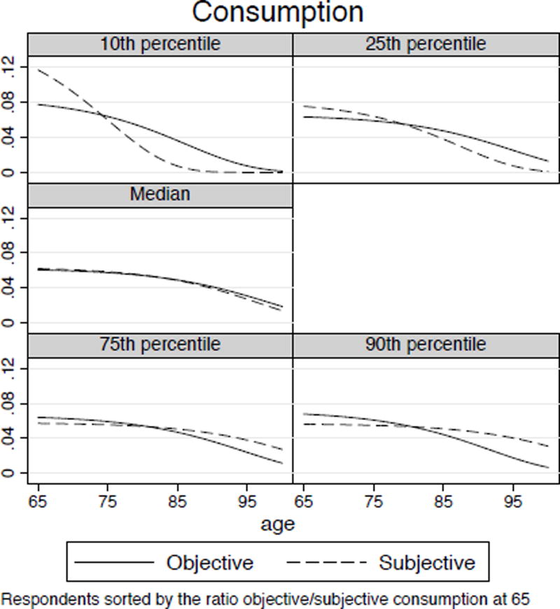
A pessimistic respondent will tend to consume her wealth more quickly than an optimistic one. One way to characterize pessimism would be to compare the ratio of initial consumption chosen under objective survival probabilities to initial consumption chosen under subjective survival probabilities. A small ratio would be a sign of pessimism (high initial consumption deriving from pessimistic subjective survival), while a high ratio would be a sign of optimism. To illustrate the difference in consumption level between pessimistic and optimistic respondents, we compute the optimal consumption path of every respondent under both objective and subjective survival expectations, order them in terms of the ratio of initial consumption and present the consumption paths of respondents assuming they hold one dollar of wealth at age 65. Figure 9 presents these paths for the 10th, 25th, 50th, 75th and 90th percentile when respondents are sorted by this ratio.

Figure 9.

Evolution optimal consumption at every age for a dollar of wealth at 65 using either subjective or objective expectations on survival probabilities.

We see in the figure that the median respondent has a consumption path that is very close to the optimal objective path. The 10th and the 25th percentiles show consumption paths of pessimistic respondents. The 10th percentile in particular illustrates a consequence of pessimism: should the respondent survive to age 85, which is highly unlikely according to subjective survival, consumption would have to be very low due to the earlier excessive consumption. The 75th and 90th percentiles show the consumption paths of optimistic persons. Consumption is initially reduced relative to optimal, objective, initial consumption and the entire consumption path is flattened. Should someone at the 90th percentile survive to advanced old age she would consume about twice as much as the optimal level.

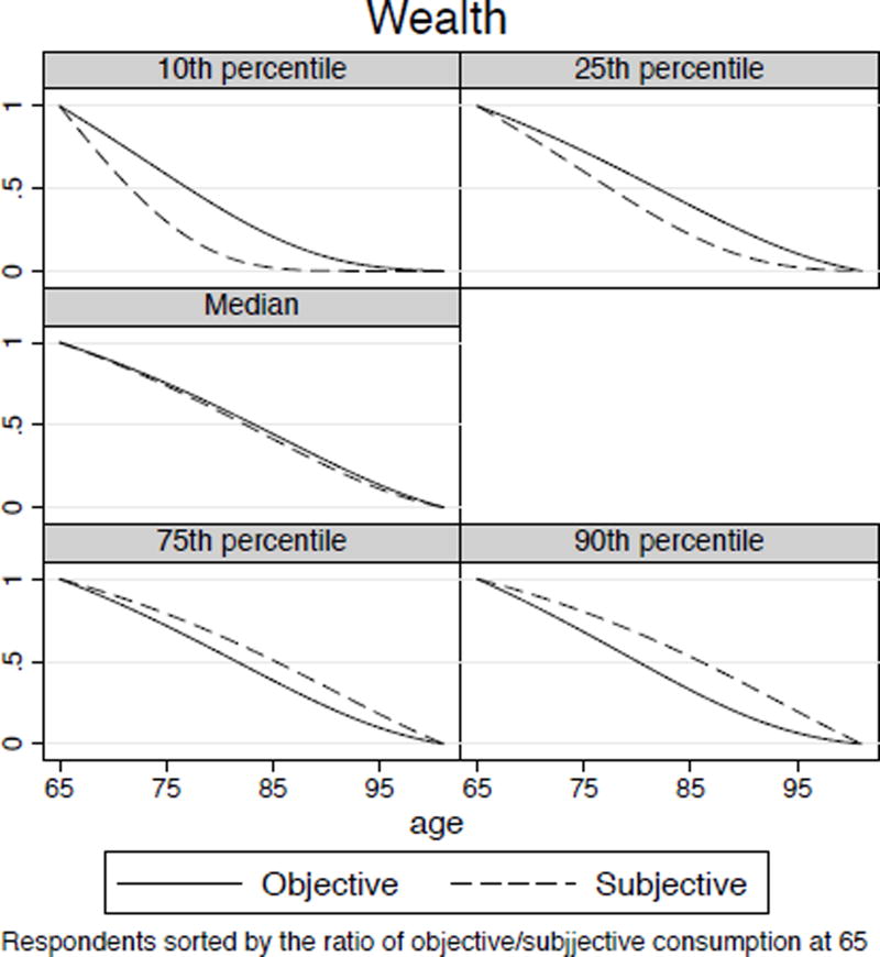
Wealth paths are affected in a similar manner by pessimism or optimism. Figure 10 presents the wealth of the same respondents. We see that the median respondents have a wealth level at every period that is just slightly below the path chosen under objective survival probability indicating a slight amount of pessimism.

Figure 10.

Evolution optimal wealth held at every age for a dollar of wealth at 65 using either subjective or objective expectations on survival probabilities.

As would be expected from the initial, excessive consumption by the pessimists, their wealth is below median; the optimists initially under-consumed and their wealth is above the median.

When subjective expectations differ from objective ones, the consumer will suffer a welfare loss by not choosing the optimal path of consumption ex ante. To get a sense of the magnitudes involved, we derive how much compensation we should give each respondent so that his expected utility at age 65 when using subjective beliefs is equal to the expected utility he could have reached had he used objective beliefs and thus implemented the optimal consumption plan. By doing this, we can also assess whether the welfare loss is larger for being pessimistic or optimistic.

Suppose subjective risk is different from objective risk. The agent will decide on the consumption path c^S(W) based on maximizing U(c^S, s^S). However, he will experience V_S(W) = U(c^S(W), s^O) which leads to a welfare loss compared to what he would have obtained had he used correct expectations: V_O(W) = U(c^O(W), s^O). It is easy to show under the preferences we use that the wealth needed relative to what the consumer has at age 65 is given by

$$W_C={\left(\frac{V_O}{V_S}\right)}^{\frac{1}{1-\sigma }}$$ (18)

where V_O is expected indirect utility using objective beliefs and the optimal plan under objective beliefs and V_S is expected utility using objective beliefs but the optimal plan chosen under subjective beliefs.

We compute the value of W_C for every respondent aged 65 or less, assuming that they do reach age 65. We present here various quantiles of the distribution of W_C according to some characteristics.⁶

Table 2 presents some quantiles of the distributions based on gender and educational level. At the median, the welfare loss amounts to 7% of wealth at age 65. This loss is larger for males than females at higher education levels. In terms of education, the welfare loss is larger for low-educated households than for college-educated households. The welfare loss is very heterogeneous, reflecting the heterogeneity in survival curves found earlier. More than 25% of respondents have welfare losses larger than 60% of their current wealth. The large losses are found all across the distribution and in particular among low-educated women.

Table 2.

Compensating wealth to correct for erroneous expectations by education

		10th	25th	Median	75th	90th
Women	Low. ed.	1.012	1.044	1.135	6.131	>10
	H. School	1.003	1.018	1.065	1.875	>10
	College	1.002	1.010	1.039	1.444	3.391
Men	Low. ed.	1.014	1.048	1.115	1.863	>10
	H. School	1.009	1.036	1.094	1.502	>10
	College	1.003	1.019	1.068	1.298	>10
Total	All levels	1.004	1.022	1.077	1.621	>10

To find whether welfare losses are larger for those who are pessimistic than for those who are optimistic, we divide the sample according to whether respondents are optimistic (i.e. with subjective life expectation larger than their objective measures) or pessimistic. Table 3 presents the results. At the median, the welfare loss is larger for pessimistic respondents (54% against 3.3%). The 75th and 90th percentile tell us that these errors can be very costly. Although being optimistic implies a welfare loss, this welfare loss is small because the initial under-spending is relatively small, and it is partially compensated by over-spending at advanced old age. Being pessimistic implies that at advanced old age spending will be very small and, hence, the marginal utility of consumption will be very high causing the discounted utility loss to be large.

Table 3.

Compensating wealth to correct for erroneous expectations by education and optimism

Pessimistic		10th	25th	Median	75th	90th
Women	Low. ed.	1.057	1.246	2.203	>10	>10
	H. School	1.015	1.184	1.712	3.882	>10
	College	1.005	1.028	1.457	2.554	>10
Men	Low. ed.	1.029	1.067	1.465	>10	>10
	H. School	1.031	1.105	1.408	>10	>10
	College	1.013	1.089	1.349	6.122	>10
Total		1.015	1.098	1.540	>10	>10

Optimistic
Women	Low. ed.	1.003	1.021	1.047	1.079	1.107
	H. School	1.001	1.009	1.023	1.052	1.071
	College	1.001	1.006	1.019	1.040	1.058
Men	Low. ed.	1.004	1.035	1.088	1.123	1.155
	H. School	1.004	1.018	1.044	1.089	1.114
	College	1.001	1.008	1.029	1.067	1.089
Total		1.001	1.011	1.033	1.067	1.099

One way to increase experienced welfare in this setting would be to provide an annuity to the respondents who spend their own wealth too quickly because of misperception in their survival probabilities. However, these same respondents who spend their wealth too fast are also those who would believe that an annuity is not a good investment. To illustrate this, we computed a fairly priced immediate fixed annuity based on the average objective survival probabilities in our sample. Denoting the yearly average survival probability to age t as ${\overline{s}}_t^O$, the yearly payout of this annuity bought at 65 for the price of one dollar is given by:

$$a=\frac{1}{{\sum }_{t=65}^{100}\frac{{\overline{s}}_t^O}{{(1+r)}^t}}=0.0877$$ (19)

So $100,000 in wealth would buy an annuity in the amount of $8,770 paid every year. Even though this annuity is actuarially fair (unlike actual annuities in the market which have load factors), 5.8% of the agents are going to prefer to self-insure based on our estimation. When we sort the respondents by the ratio of initial consumption under objective and subjective expectations, those who prefer self-insurance are all concentrated below the 12th percentile of this ratio, and are precisely those who would benefit the most from the annuity. We estimate that another 45.6% of respondents would buy an annuity at a fair price despite having pessimistic expectations. This could result in an important welfare gain. We know however that annuities found in the market place are not actuarially fair. For instance, Mitchell et al. (1999) reported that the annuities on the market had expected present value about 20% below the actuarially fair present value. In our framework, this would lead to a payout of 0.0701, which roughly corresponds to the market payout of the immediate fixed annuity at the time of writing. Using this payout, we find that 15.5% of respondents would prefer to self-insure themselves. These respondents are concentrated below the 38th percentile and are all pessimistic respondents. No respondents in the 10th percentile and below would choose the annuity.

5.1 Social Security

In reality, most households can count on annuity income from a public pension such as Social Security to finance consumption in case they run out of wealth. Hence, estimates of the welfare loss which do not account for annuities may exaggerate the effect of longevity risk. To illustrate this, we perform the same exercise accounting for annuity income. By definition, annuity income is received at every time period if an individual is alive. Denote this amount SS. Optimal consumption is chosen to satisfy Equation 16 as long as wealth is positive. Given that we assume Rβ = 1, consumption declines with age under Equation 16. But if wealth becomes zero, consumption must equal SS. To avoid a discontinuity in consumption (and in marginal utility) optimal consumption under equation 16 must reach SS just when wealth becomes zero. Thus Equation 14 becomes

$$W=\sum _{t=0}^N{R}^{-t}(c_t^j-SS)\mathrm{s}.\mathrm{t}. c_t^j\ge SS\forall t$$ (20)

where N is the age at which wealth is exhausted. Consumption is governed by Equation 16 for t < N and C_t = SS for t > N. We solve this problem by calculating numerically the optimal consumption paths under objective and subjective survival that satsify the first-order conditions and the constraints.

We assume that respondents annuitize part of their initial unit of wealth at the yearly payout computed in Equation 19. Since we normalize by wealth at age 65, we look at HRS data for guidance on the relevant range for SS, where we define SS as the sum of Social Security income and private annuity income. We vary the ratio $\frac{SS}{W}$ from 0 to 0.10, which is the observed range for about 75% of our sample. The median value is about 0.03; that is, annual annuity income is approximately 3% of total wealth for the median household. Equation 18 does not hold anymore, so we use numerical methods to evaluate the initial compensating wealth, W_C, for every respondent. Results are reported in Table 4.

Table 4.

Median compensating wealth to correct for erroneous expectations by education for various level of SS.

	$\frac{SS}{W}$	0	0.020	0.040	0.060	0.080	0.100
Women	Low. ed.	1.135	1.067	1.048	1.035	1.027	1.021
	H. School	1.065	1.051	1.035	1.024	1.018	1.014
	College	1.039	1.034	1.025	1.018	1.014	1.011
Men	Low. ed.	1.115	1.070	1.046	1.033	1.026	1.021
	H. School	1.094	1.047	1.032	1.024	1.019	1.015
	College	1.068	1.043	1.026	1.018	1.014	1.011
Total	All levels	1.077	1.047	1.032	1.023	1.018	1.014

When annuity income is equal to 10% of initial wealth, the median welfare loss is 1.4% compared to 7.7% when no annuity income is present. Thus annuity income can protect individuals from erroneous mortality beliefs, which in our data is most evident among those with low levels of education. For example, the welfare loss among women lacking a high school education is reduced from 13.5% of total wealth to 6.7% when the ratio of annuity income to wealth increases from zero to 2%. Despite the presence of Social Security, however, the welfare loss is substantial for some individuals.

6 Conclusion

In this paper, we estimate jointly subjective and objective survival curves where there is rounding on subjective reports of perceived mortality risk. We use data from the Health and Retirement Study covering a 16 year period, in particular mortality dates and measurements of subjective survival to a target age. Hence, this framework allows us to investigate whether in aggregate respondents correctly perceive their mortality risk. Instead of using life-tables as a benchmark, we use their actual mortality experience which we show is important because both non-response and survey design make inappropriate the life-table as a benchmark. Since we obtain individual objective and subjective survival curves, we are also able to obtain a full distribution of joint curves which allows us to assess distributional issues rather than look at aggregate predictions. For example, we can investigate whether particular sub-groups are too optimistic or pessimistic regarding their own mortality risk. While doing this exercise, we adjust for rounding which is important for investigating the distribution of individual survival curves.

We find that at the median, both men and women are slightly optimistic regarding their survival prospects. Other subgroups such as black, more educated respondents, and respondents from younger cohorts are also optimistic regarding their survival prospects. It is important to note that these comparisons do not involve making assumptions about cohort or composition effects because we look at the mortality experience of the same respondents who answered subjective probability questions. The case of smokers is particularly interesting. While non-smokers appear to correctly perceive their mortality risk, smokers are too optimistic. Finally, we compute the welfare loss of using erroneous beliefs in retirement when it comes to spending down wealth. This exercise shows that welfare loss can be large and more so for pessimistic expectations. Pessimistic expectations can be a barrier for annuitization for a small but important fraction of the population.

Individual survival curves can be used directly in the context of economic models. They are smooth, non-degenerate, and with finite life expectancy. One interesting exercise would be to investigate how the estimation of preferences in life-cycle models of economic decision making is impacted by using subjective rather than objective individual survival curves.

Appendix

A Details of the derivations

A.1 Derivation of the expected survival probability

We can derive the expected survival probability from age a to age t as follows:

$$S_a(t|{\mathit{x}}_{\mathit{i}})=\int \frac{S(t|{\mathit{x}}_{\mathit{i}},\nu )}{S(a|{\mathit{x}}_{\mathit{i}},\nu )}f(\upsilon |T>a)d\upsilon$$

which, given that

$$f(\upsilon |T>a)=S(a|{\mathit{x}}_{\mathit{i}},\nu )f(\upsilon )/S(a|{\mathit{x}}_{\mathit{i}})$$

yields

$$S_a(t|{\mathit{x}}_{\mathit{i}})=\frac{1}{S(a|{\mathit{x}}_{\mathit{i}})}\int S(t|{\mathit{x}}_{\mathit{i}},\nu )f(\upsilon )d\upsilon =\frac{S(t|{\mathit{x}}_{\mathit{i}})}{S(a|{\mathit{x}}_{\mathit{i}})}.$$

We can use known results for the integration of the hazard over the gamma distribution to obtain a closed-form solution (see for instance Cameron and Trivedi, 2005, pp. 615–616),

$$S_a(t|{\mathit{x}}_{\mathit{i}})={\left(\frac{\delta +\mathrm{\Lambda }(a|{\mathit{x}}_{\mathit{i}})}{\delta +\mathrm{\Lambda }(t|{\mathit{x}}_{\mathit{i}})}\right)}^{\delta }.$$ (21)

A.2 Distribution of the frailty terms for respondents aged a

Given that we need the distribution of survival probabilities to age t given survival to a in order to model rounding, denote the conditional distribution of subjective survival rates F_s(s^S|T > a, x_i). To obtain an expression for this distribution, we can use F_νs(υ|T > a, x_i), the distribution of ν^S conditional on surviving to time a:

$$F_s(s^S|T>a,{\mathit{x}}_{\mathit{i}})=1-F_{\nu s}(-\frac{\text{ln }{s}^S}{{\mathrm{\Lambda }}_a^S(t|{\mathit{x}}_{\mathit{i}})}|T>a,{\mathit{x}}_{\mathit{i}}).$$

This is due to the fact that for two random variables (Y, X), if Y = g(X), then F(y) = F_X(g⁻¹(y)).

Remember that the Gamma distribution 𝒢(c, d) is given by

$$F(x)={\int }_0^x\frac{d^{-c}{x}^{c-1}\text{ exp }(-\frac{u}{d})}{\mathrm{\Gamma }(c)}\mathrm{d}u$$

and this distribution has an expected value of cd and a variance of cd². Notice that if d = 1/δ and c = δ, the distribution has a unit expectation and a variance of 1/δ.

Let d = δ⁻¹ such that ν^S at a = 0 is distributed gamma 𝒢 (δ, d). Given the value of d, ν^S has unit expectation. The distribution of ν^S conditional on being alive at age a is:

$$\begin{gathered} F_{\nu s}(\nu |T>a,{\mathit{x}}_{\mathit{i}})=\frac{1}{S^S(a|{\mathit{x}}_{\mathit{i}})}{\int }_0^{\nu }{S}^S(a|{\mathit{x}}_{\mathit{i}},u)f(u)\mathrm{d}u \\ =\frac{1}{S^S(a|{\mathit{x}}_{\mathit{i}})}{\int }_0^{\nu }\text{exp}(-u{\mathrm{\Lambda }}^S(a|{\mathit{x}}_{\mathit{i}}))\frac{d^{-\delta }{u}^{\delta -1}\text{ exp}(-\frac{u}{d})}{\mathrm{\Gamma }(\delta )}\mathrm{d}u \\ =\frac{d^{-\delta }}{S^S(a|{\mathit{x}}_{\mathit{i}})}{\int }_0^{\nu }{u}^{\delta -1}\frac{\text{exp}(-u({\mathrm{\Lambda }}^S(a|{\mathit{x}}_{\mathit{i}})+\delta ))}{\mathrm{\Gamma }(\delta )}\mathrm{d}u. \end{gathered}$$

For the sake of exposition, let k = 1/(Λ^S(a|x_i) + δ), and remember that S^S(a|x_i) = (d/k)^−δ

$$\begin{gathered} F_{\nu s}(\nu |T>a,{\mathit{x}}_{\mathit{i}})=\frac{d^{-\delta }}{S^S(a|{\mathit{x}}_{\mathit{i}})}{\int }_0^{\nu }{u}^{\delta -1}\frac{\text{exp}(-\frac{u}{k})}{\mathrm{\Gamma }(\delta )}\mathrm{d}u \\ =\frac{1}{S^S(a|{\mathit{x}}_{\mathit{i}})}\frac{d^{-\delta }}{k^{-\delta }}{\int }_0^{\nu }{k}^{-\delta }{u}^{\delta -1}\frac{\text{exp}(-\frac{u}{k})}{\mathrm{\Gamma }(\delta )}\mathrm{d}u \\ ={\int }_0^{\nu }\frac{k^{-\delta }{u}^{\delta -1}\text{ exp}(-\frac{u}{k})}{\mathrm{\Gamma }(\delta )}\mathrm{d}u. \end{gathered}$$

Then it follows directly that F_νs(υ|T > a, x_i) is distributed gamma 𝒢 (δ, k), leading to an expected value of $\frac{\delta }{{\mathrm{\Lambda }}^S(a|{\mathit{x}}_{\mathit{i}})+\delta }$ and a variance of $\frac{{\delta }^2}{{({\mathrm{\Lambda }}^S(a|{\mathit{x}}_{\mathit{i}})+\delta )}^2}$.

This makes explicit that the mean and variance of the frailty term decreases as age increases, as the integrated hazard is expected to increase with age, leading to a decrease in k.

References

- Cameron AC, Trivedi PK. Microeconometrics: Methods and Applications. Cambridge University Press; New York, NY: 2005. [Google Scholar]
- De Bruin WB, Fischhoff B, Millstein SG, Halpern-Felsher BL. Verbal and Numerical Expressions of Probability: It’s a Fifty-Fifty Chance. Organizational Behavior and Human Decision Processes. 2000;81(1):115–31. doi: 10.1006/obhd.1999.2868. [DOI] [PubMed] [Google Scholar]
- DeNardi M, French E, Jones JB. Why Do the Elderly Save? The Role of Medical Expenses. Journal of Political Economy. 2010;118(1):39–75. [Google Scholar]
- Dominitz J, Manski CF. Expected Equity Returns and Portfolio Choice: Evidence from the Health and Retirement Study. Journal of Behavioral Decision Making. 2007;5(2–3):369–79. [Google Scholar]
- Gan L, Hurd MD, McFadden D. Individual Subjective Survival Curves. In: Wise DA, editor. Analyses in Economics of Aging. I. University of Chicago Press; Chicago: 2005. pp. 377–411. [Google Scholar]
- Hamermesh D. Expectations, Life Expectancy, and Economic Behavior. Quarterly Journal of Economics. 1985;100(2):389–408. [Google Scholar]
- Hubbard G, Skinner J, Zeldes SP. Precautionary Saving and Social Insurance. Journal of Political Economy. 1995;103(2):360–399. [Google Scholar]
- Hurd MD, McGarry K. Evaluation of the Subjective Probabilities of Survival in the Health and Retirement Study. Journal of Human Resources. 1995;30:268–292. [Google Scholar]
- Hurd MD, McGarry K. The Predictive Validity of Subjective Probabilities of Survival. The Economic Journal. 2002;112:966–985. [Google Scholar]
- Hurd MD, Smith JP, Zissimopoulos JM. The Effects of Subjective Survival on Retirement and Social Security Claiming. Journal of Applied Econometrics. 2004;19(6):761–775. [Google Scholar]
- Hurd MD. Mortality Risk and Bequests. Econometrica. 1989;57:779–813. [Google Scholar]
- Kleinjans KJ, van Soest A. Rounding, Focal Point Answers and Nonresponse to Subjective Probability Questions. Journal of Applied Econometrics 2013 [Google Scholar]
- Khwaja A, Sloan F, Chung S. The Relationship Between Individual Expectations and Behaviors: Mortality Expectations and Smoking Decisions. Journal of Risk and Uncertainty. 2007;35:179–201. [Google Scholar]
- Lichtenstein S, Slovic P, Fischoff B, Layman M, Combs B. Judged Frequency of Events. Journal of Experimental Psychology: Human Learning and Memory. 1978;4(6):551–578. [PubMed] [Google Scholar]
- Manski CF, Molinari F. Rounding Probabilistic Expectations in Surveys. Journal of Business and Economics Statistics. 2010;28(2):219–231. doi: 10.1198/jbes.2009.08098. [DOI] [PMC free article] [PubMed] [Google Scholar]
- Mitchell OS, Poterba JM, Warshawsky MJ, Brown JR. New Evidence on the Money’s Worth of Individual Annuities. American Economic Review. 1999;89(5):1299–1318. [Google Scholar]
- Salm M. Subjective mortality expectations and consumption and saving behaviors among the elderly. Canadian Journal of Economics. 2010;43(3):1040–1057. [Google Scholar]
- Scholz JK, Seshadri A, Khitatrakun S. Are Americans Saving ‘Optimally’ for Retirement? Journal of Political Economy. 2006;114(4):607–643. [Google Scholar]
- Yaari ME. Uncertain Lifetime, Life Insurance, and the Theory of the Consumer. Review of Economic Studies. 1965;32:137–150. [Google Scholar]
Associated Data
This section collects any data citations, data availability statements, or supplementary materials included in this article.