Significance
Covariance analysis of protein sequence alignments can predict structure and function from sequence alignments alone. Current methodologies typically assume that sequences are independent, notwithstanding their phylogenetic relationships. This corruption constrains the alignments for which covariance analysis can be used. It is critically important to control for phylogeny and understand how phylogeny contaminates signal. This paper presents a mathematical analysis that argues that there is a distinctive signature of phylogeny in the covariance matrix, allowing us to identify modes that are corrupted by phylogeny. This signature is present in large protein sequence alignments, explaining recent covariance analyses, and provides an important step toward decoupling phylogenetic effects from biologically meaningful interactions.
Keywords: power law, sequence covariance, phylogeny, protein, structure prediction
Abstract
Covariance analysis of protein sequence alignments uses coevolving pairs of sequence positions to predict features of protein structure and function. However, current methods ignore the phylogenetic relationships between sequences, potentially corrupting the identification of covarying positions. Here, we use random matrix theory to demonstrate the existence of a power law tail that distinguishes the spectrum of covariance caused by phylogeny from that caused by structural interactions. The power law is essentially independent of the phylogenetic tree topology, depending on just two parameters—the sequence length and the average branch length. We demonstrate that these power law tails are ubiquitous in the large protein sequence alignments used to predict contacts in 3D structure, as predicted by our theory. This suggests that to decouple phylogenetic effects from the interactions between sequence distal sites that control biological function, it is necessary to remove or down-weight the eigenvectors of the covariance matrix with largest eigenvalues. We confirm that truncating these eigenvectors improves contact prediction.
Approaches to biological sequence analysis typically assume that mutations at different sites are independent of each other, although this approximation is clearly limited. Indeed, covariation between sequence distal positions is important for predicting RNA secondary structure (1), where Watson–Crick base-pairing rules create strong covariance signals that can be detected by straightforward methods. In contrast, for proteins, the signal is less strong, and for many years it was unclear whether any remnant of molecular phenotypes such as protein structure is imprinted on covarying sequence positions (2–4).
Recently, with the growth of protein sequence databases (5) and the introduction of sophisticated analyses (6–8), it has become clear that covariance analysis of protein sequences can yield exciting biological insights in a wide range of contexts (9–27). In general a set of homologous protein sequences is constrained by protein structure and function, and with sufficient data it is possible to tease out the nature of these constraints and make biologically relevant predictions (12, 13, 16, 28–32).
An important consideration that limits our ability to infer sets of covarying residues is sequence phylogeny, i.e., the relatedness structure of the data samples (33–35). If some population subgroups are more closely related, then part of the covariation observed in the data will be of purely phylogenetic origin, unrelated to molecular phenotypes such as structure or function (36–41). In population and medical genetics features such as geographical population structure are known to affect the degree of covariance observed between sequences. (42–44).
This raises the question of whether, given aligned protein sequences of length , it is possible to distinguish covariance due to phylogeny from that caused by molecular phenotypes (36–41). Here, we analyze a simple theoretical model of molecular evolution and use the tools of random matrix theory (RMT) to develop a theory for the covariance when both phylogeny and structural constraints are present. We show that phylogenetic covariance is distinguished by a power law tail of large eigenvalues, which is essentially independent of phylogenetic details, depending only on the average branch length and the number of branching events or generations.
Thus motivated, we turn to data and find that the eigenvalue distributions of covariance matrices from large protein sequence alignments (MSAs) have power law tails. This suggests a strategy for cleaning the covariance matrix that at least partly controls for confounding phylogenetic effects: removing the power law tail representing those modes that are most strongly corrupted by phylogeny. For several protein families, we show that contact prediction accuracy improves by excluding those eigenvectors that correspond to the largest eigenvalues. It is interesting to note that the commonly used method of inverting the sample covariance matrix similarly down-weights the largest eigenvalues and up-weights the smallest ones. Our analysis therefore gives an alternative rationalization for why direct coupling analysis (DCA) has proved so successful at inferring true contacts in proteins from sequence data alone. More generally, this eigenvalue power law will occur in any dataset where the samples have a similar hierarchical relationship.
Results
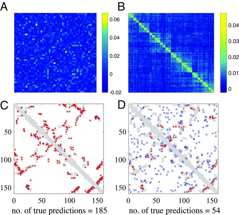
Molecular phenotypes cause covariance between sequence positions (columns) of the MSA matrix , while phylogeny causes covariance between sequences (rows) of . Covariance from either source will appear in both the residue covariance matrix and the sequence covariance matrix . This is because and contain the same information; they have the same nonzero eigenvalues, and their eigenvectors and are related by and . Analyses of protein sequence data typically attribute the detected covariance signal to interactions between sequence positions. This can be misleading: Fig. 1 A and B shows and for a simulated dataset where phylogeny is the only source of covariance. Note that contains isolated high-scoring residue pairs caused by phylogeny, which could be erroneously interpreted to be caused by molecular phenotypes.
Fig. 1.
(A and B) The covariance matrices (A) and (B) for sequences simulated with just phylogeny. Note that has isolated large entries that could be interpreted to indicate interactions between pairs of sequence positions, although none exist in the simulation. (C) In simulations where the contact map of dihydrofolate reductase (DHFR) is used to generate interactions (gray), causal interactions are detected well by the largest 200 off-diagonal pairs of in the absence of phylogeny (red, true interaction; blue, false positive). (D) The addition of phylogeny to these simulations confounds the signal.
What happens if there are structural interactions between specific residue pairs in the simulation? In Fig. 1 C and D we compare the true interactions (gray) with the top 200 scoring pairs from covariance matrices for sequences simulated without (Fig. 1C) and with (Fig. 1D) phylogeny. Without phylogenetic corruption, predictions are correct; whereas with phylogeny this reduces to . The essential question is to find a way to disentangle phylogenetic and phenotypic (e.g., structural) covariance from matrices that contain a superposition of both (e.g., Fig. 1D). To address this, we first analyze the covariance signal produced by sequences for which the only source of covariance is phylogeny and then ask whether we can distinguish this signal when both phylogenetic and structural correlations are present.
Phylogenetic Covariance.
To understand the signature of phylogenetic covariance, we consider a Markov model where mutations occur at random and different sites evolve independently. The process starts with a random sequence of length , drawn from a -letter alphabet, which undergoes a series of mutation and duplication events dictated by a user-imposed phylogeny with branching events. This generates an alignment of simulated sequences. Population structure changes the eigenvalue spectrum of the resulting covariance matrix. To see this, consider the simplest phylogeny, consisting of a single branching event with equal-length branches. The true covariance matrix , i.e., the covariance matrix of the distribution the samples are drawn from, follows by calculating the covariance between the resulting sequences and . Since this is a stationary Markov process, the covariance between two sequences separated by mutations, which we denote , is , which yields
| [1] |
where the last equality specializes to a binary alphabet. A phylogeny with a single branching event has the true covariance matrix
| [2] |
As the mutation rate , note that . This means that , i.e., the sequences are uncorrelated, and phylogenetic influence is negligible. More generally, as the number of branching events or generations increases, we find that is composed of nested squares that correspond to each branching event. This yields distinct eigenvalues , with , except for the two largest eigenvalues, which have (Supporting Information). These relationships imply that the eigenvalues follow the power law
| [3] |
where is the rank, and is a function of . Under the influence of phylogeny, the maximum eigenvalue increases exponentially with the number of branching events . Note that there is a precise threshold at , which given Eq. 1 for implies , above which this power law behavior occurs.
Finite-Sampling Effects.
We have thus seen that phylogeny produces a striking signature in the covariance matrix. However, because the number of MSA sequences is limited, this signature will be affected by finite sampling—the sample covariance matrix will contain large entries purely by chance. We use RMT to develop a quantitative characterization of the effect on the corresponding eigenvalue distribution. Consider independent sequences of length , with amino acids drawn uniformly at random. The probability distribution of the sample eigenvalues follows the Marčenko–Pastur (MP) distribution
| [4] |
where (45). Our simulations confirm that the histogram of eigenvalues of sequences simulated without phylogeny or structural interactions is well described by this analytical formula (Fig. 2A). As increases, Eq. 4 implies that this distribution sharpens around . RMT further predicts how Eq. 4 generalizes to describe the eigenvalue distribution of the sample covariance matrix for any true covariance matrix , such as those caused by phylogeny. We start with the Stieltjes transform,
| [5] |
where is the cumulative distribution function of , the limiting eigenvalue distribution of . Marčenko and Pastur (45) used the method of characteristics to relate to , the cumulative eigenvalue distribution of the true covariance matrix , yielding
| [6] |
This equation describes the effects of finite sampling. If the true eigenvalues cluster at/near unity, this will result in the MP distribution of Eq. 4. For phylogeny, the eigenvalues of are drawn from a discrete distribution, so (46), where follows the power law of Eq. 3. Eq. 6 describes how finite sampling smoothens out this discrete distribution.
Fig. 2.
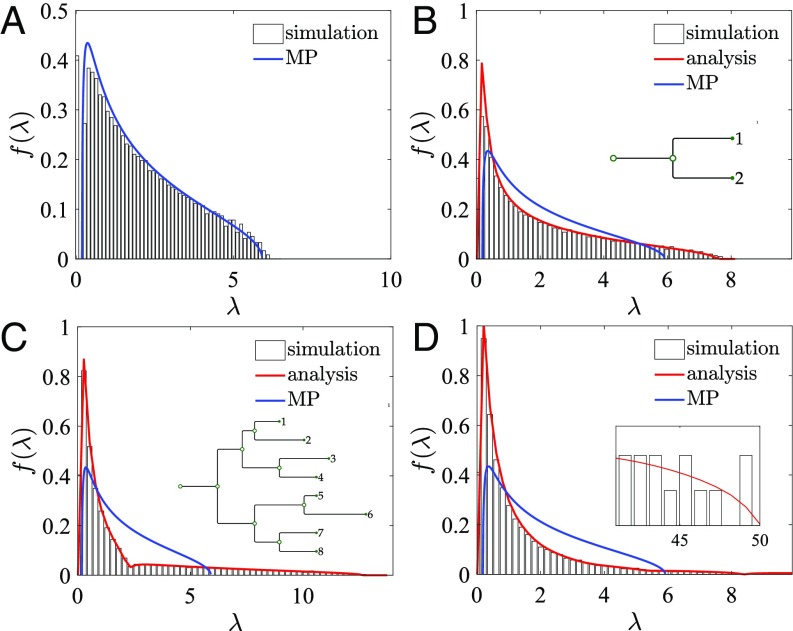
(A) Eigenvalue distributions of sequences with residues, drawn from a model with . The eigenvalues of the sequence covariance matrix (bars) match the classical MP distribution (blue curve). (B) Here initial sequences are simulated along a tree with equal branch lengths and a single branching event, with mutations per branch. (C) Here initial sequences are evolved with branching events (Inset); branch lengths are drawn from a Poisson distribution with mean 10. (D) Here initial sequences are evolved with branching events and branch lengths drawn from a half-normal distribution with mean 10 (Inset, eigenvalue tail). In each case, the histogram of eigenvalues (averaged over 200 runs) matches the analytical solution (red curve), not the classical MP distribution (blue curve).
Fig. 2B shows how the eigenvalue distribution changes if the sequences follow our simplest phylogeny, where (Eq. 2) has eigenvalues . Alignments of sequences were simulated with mutations per branch. The shape of the eigenvalue distribution differs significantly from that of the MP distribution (blue curve). RMT allows us to predict this spectrum using Eq. 6, which becomes
The inverse Stieltjes transform, given by the positive imaginary part of , analytically describes the expected eigenvalue distribution of . This is used to plot the red curve in Fig. 2B, which shows excellent quantitative agreement with the simulation, unlike the MP distribution shown in blue. As the number of branching events increases we simply use our exact formulas (Supporting Information) for the true eigenvalue distributions in Eq. 6 to compute the expected distribution.
Analysis of Inhomogeneous Phylogenies.
Real phylogenetic trees are inhomogeneous, with branches of different lengths. Our framework naturally extends to this setting. Fig. 2 C and D shows the eigenvalue distributions of trees drawn from different distributions; Fig. 2C has three branching events with branch lengths drawn from a Poisson distribution, while Fig. 2D has seven branching events with branch lengths drawn from a half-normal distribution. Note that the eigenvalue distribution broadens as the number of branching events increases, reflecting that the maximum true eigenvalue is .
For inhomogeneous phylogenies we discovered that analytical solutions follow a simple rule. Consider a phylogeny with branch lengths drawn from a distribution with mean and bounded variance; the eigenvalue distribution is then well approximated by the eigenvalue distribution for the tree with all branch lengths equal to and the same number of branching events. The red curves in Fig. 2 C and D show that this prediction fits the simulated data closely. To derive the result, we consider a phylogeny with and branch lengths drawn from a Poisson distribution with mean , so that . If , then the eigenvalues of the true covariance matrix are . Applying Eq. 6 we find
Examining the summands, we note that
where
In the limit of large the dependence on the tree parameters and simplifies, so that
This approximation, valid for large , allows us to write
Hence the Stieltjes transform for the inhomogeneous tree is equal to the Stieltjes transform for a homogeneous tree with the mean of the distribution the branch lengths are drawn from. This result can be generalized for any arbitrary distribution and phylogenetic tree topology (Supporting Information). This result about inhomogeneous phylogenies is important as it extends our analysis methods to more realistic phylogenies, implying that the power law tail of large eigenvalues described above is general.
Phenotypic Covariance.
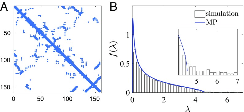
The eigenvalue spectrum for phenotypic covariance depends on how phenotype couples the residues to each other. While this will differ for different phenotypes, recent work has focused on using covariance analysis to predict contacts in tertiary protein structure (11, 13, 14, 16–18). If we consider interactions drawn from a protein contact map, what covariance is caused? For an alphabet with , the correlation between two residues that interact with strength is given by , which saturates as increases so that the resulting correlation does not exceed unity. With multiple interactions and a larger alphabet, the situation is more complex; however, we can use simulations to characterize the sample covariance matrix and corresponding eigenvalue distribution. We first simulate sequences without phylogeny, using a simple Markov model with nonzero residue couplings at locations dictated by protein contact maps. These couplings were chosen uniformly from the interval [−5, 5]. With the 784 interactions of Fig. 3A, the eigenvalue distribution of the sample covariance matrix is described well by the MP distribution (Fig. 3B). This empirical observation suggests that the eigenvalues of the true covariance matrix are all of similar size, suggesting that structural interactions do not lead to an eigenvalue power law. While real proteins will also have other phenotypic interactions, this model provides a relevant starting point.
Fig. 3.
Simulations with just structural interactions. Here 4,096 sequences are simulated without phylogeny, with structural interactions taken from the contact map of DHFR with strengths uniformly distributed on [−5, 5]. A shows the interaction matrix, and B is the spectrum of the covariance matrix of the resulting sequence alignment. B, Inset shows the upper edge of the eigenvalue distribution in more detail; compare with Fig. 2D.
Phylogenetic vs. Structural Covariance.
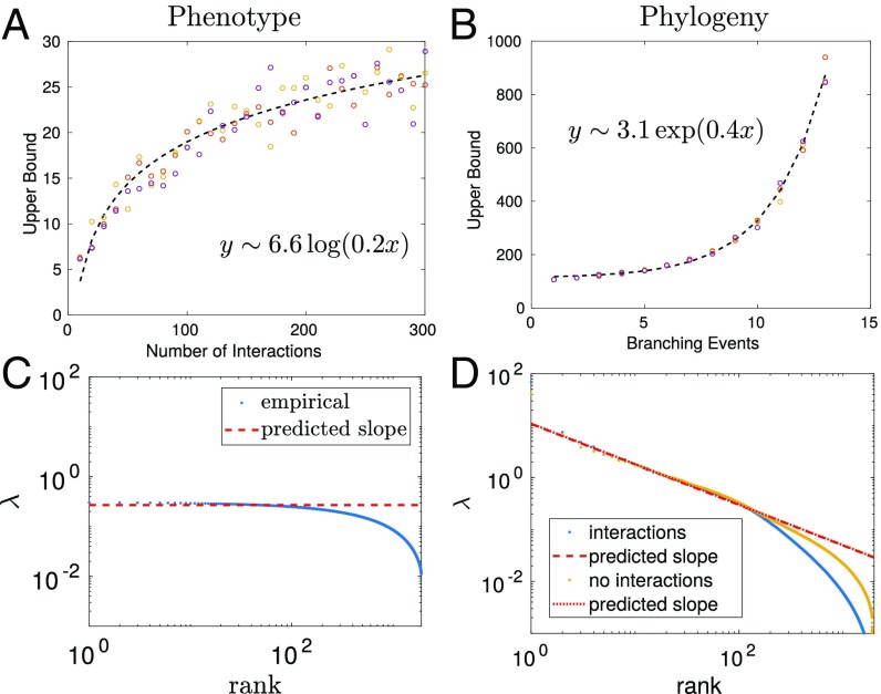
Crucially, this model suggests that there are strikingly different signatures between the covariance matrix expected from phylogeny and that expected for interactions caused by residue contacts. If only structural interactions are present, the limiting behavior of the maximum eigenvalue saturates logarithmically as a function of the number of interactions (Fig. 4A). In contrast, Fig. 4B shows that the maximum eigenvalue caused by phylogeny increases exponentially as the sequences undergo more duplication events. Moreover, Fig. 4C shows a log–log plot of the eigenvalues as a function of rank for our simulations with just phenotypic interactions (Fig. 3); the data are well fitted by a line of slope zero reflecting the absence of the power law.
Fig. 4.
(A and B) Largest eigenvalue obtained in simulations with (A) only structural interactions with strength 1.0 and (B) only phylogeny. Lines of best fit are shown. (C) Eigenvalue distribution obtained in simulations from Fig. 3 with just structural interactions, where the predicted slope is zero. (D) Comparison of eigenvalue distributions obtained in simulations with (yellow) phylogeny and (blue) phylogeny and structural interactions. The presence of interactions does not alter the power law, but does affect the small eigenvalue behavior. The lines of best fit are constrained using , where is from Eq. 1.
To probe these signatures further, we use simulations with a controlled mix of phylogeny and structural interactions. Fig 4D shows that the spectra for simulations with just phylogeny and simulations with both phylogeny and 200 random structural interactions obey the same power law. In both cases the upper power law tail follows (red line). With interactions, the lower extent of the power law is diminished; the blue curve in Fig. 4D drops off before the yellow curve. Importantly, these two spectra diverge only outside the power law regime, implying that phylogeny dominates those modes that follow the power law.
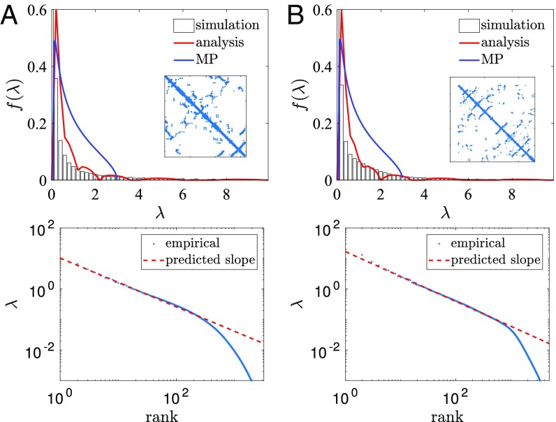
These simulations therefore suggest that interactions between residues affect the smallest eigenvalues, while phylogeny affects the largest eigenvalues, giving a potential mechanism for distinguishing the effects of phylogeny. Intuitively, this could arise because interactions between residues make it less likely that mutations at those sites will be accepted, reducing the effective mutation rate of these residues and hence affecting eigenvectors with low eigenvalues. In Fig 5 we simulate sets of sequences with both phylogeny and structural interactions from two different protein contact maps and obtain similar results to those in Fig 4D. In contrast to Fig. 3, we find that the eigenvalue distributions of the resulting sequence alignments are not MP, but are well fitted by our analytic approach. The red curves in Fig. 5 A and B are each found using the phylogenetic parameters from the power law fits in Fig. 5 C and D, respectively.
Fig. 5.
Simulations with phylogeny and interactions. Here sequences are simulated with phylogeny and interactions taken from the contact map of (A) DHFR, using , and (B) Trypsin, using . A and B, Top show the histograms of eigenvalues, compared with the MP distribution (blue curve); Insets show the contact maps. These values are used to compute the analytical distributions (red curves) which match the data well. A and B, Bottom show log–log plots of the eigenvalues as a function of rank. The predicted slope is calculated from the value of using Eq. 1 in each case and provides an excellent fit.
Eigenvalue Spectra of Protein Sequence Data.
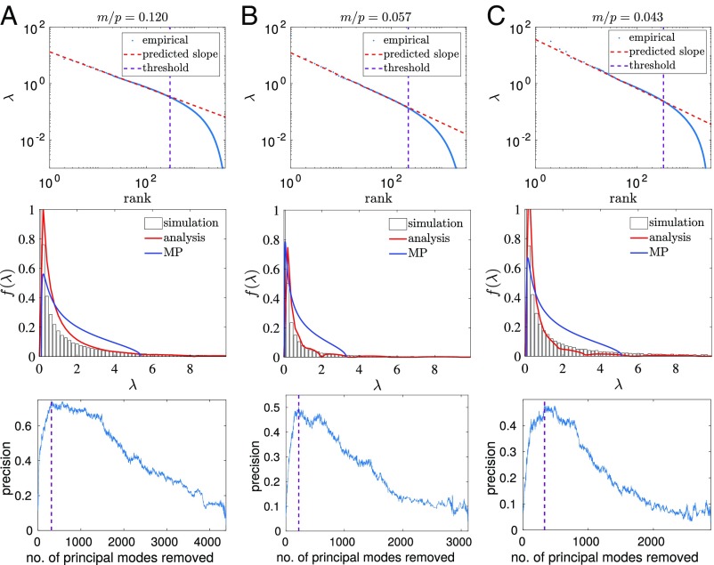
Given the vastly different signatures in the eigenvalue distributions expected from phylogeny and structural interactions, it is of great interest to see whether such signatures arise in protein sequence data. To probe this, we choose three representative protein families for which covariance analysis has been shown to yield accurate contact predictions. In Fig. 6 A–C, Top we show that the eigenvalue distributions follow a power law in each case, as predicted by our theory. Furthermore, as for the simulated data, Fig. 6 A–C, Middle shows that the phylogenetic parameters extracted from the power fitted in each case provide a closer fit (red curves) to the eigenvalue distribution than to the MP distribution (blue curves).
Fig. 6.
Protein sequence alignments follow the power law, and moreover spectral deviation from the power law can be used to deconvolve the influence of phylogeny from the covariance matrix, and facilitate contact prediction. A–C show analysis of protein sequence data from (A) Trypsin, (B) DHFR, and (C) TRML-HAEIN, a knotted tRNA-methyltransferase. In A–C, Top we show that the eigenvalues of each protein sequence alignment follow a power law. The purple dashed line indicates the point at which the spectrum deviates from this power law, indicating a threshold above which phylogeny dominates the spectrum. The parameter is inferred from this power law using the equation , where and is given by Eq. 1. The inferred values of are used to plot the red lines in A–C, Middle, which provide a good fit to the empirical spectral distributions. A–C, Bottom show that the phylogenetic threshold, derived from A–C, Top, provides an excellent indication of which modes should be removed from the covariance matrix to deconvolve the influence of phylogeny and dramatically improve contact prediction using just the covariance matrix.
Cleaning Protein Spectra.
The analysis of simulated data suggests that the effects of phylogeny can be diminished by removing large modes of the covariance matrix and enforcing the constraint that the remaining eigenvalues are all of the same size. Namely, instead of the full covariance matrix from the sequence alignments, we propose truncating the highest modes,
where . Fig. 6 shows the results of this approach for contact prediction. For each protein, the slope of the power law fit in Fig. 6 A–C, Top is used to estimate the phylogenetic parameters required for the analytical solution in Fig. 6 A–C, Middle (red curve). The point at which the eigenvalues deviate from the power law fit in Fig. 6 A–C, Top (purple dashed line) is used to determine which modes are dominated by phylogeny and should be truncated from the outer product expansion of the sample covariance matrix. Fig. 6 A–C, Bottom shows how well different truncations do at contact prediction; the purple dashed line reflects the threshold found from the power law fit and is near optimal in all cases. This phenomenology is entirely consistent with the notion that the modes corresponding to the large eigenvalues reflect the phylogenetic relatedness of the aligned sequences.
Discussion
This paper was motivated by recent advances (9–14, 16, 21) in predicting protein structure and function from the covariation of sequences, a strategy that has been successful for predicting RNA secondary structure for some time (1, 35). A major confounding effect in both situations is the effect of phylogeny, which introduces correlations between residues (30, 36, 38). The correlations due to structure/function and phylogeny must be disentangled for accurate prediction.
The primary accomplishment of this paper is to identify a feature of the eigenvalue distribution of protein covariance matrices (the power lawtail) that distinguishes covariance due to phylogeny from that caused by structural interactions. The presence of power law tails in the data from diverse protein families allows us to develop an initial approach to deconvolving structural interactions from the covariance that results from sequence phylogeny alone. Our finding that the largest modes of the covariance matrix are dominated by phylogeny suggests an alternative rationalization for the matrix inversion step that enabled features of protein structure and function to be predicted from covariance analysis of large protein sequence alignments. Furthermore the resulting cleaned covariance matrix can be used as input for other inference approaches (9–12, 18, 19, 21).
A further result is a general understanding of how phylogenetic effects impact sequence covariation in different regions of parameter space. Depending on the sequence length and the average branch length , there is a parameter regime where the covariance matrix does not feature a power law tail of large eigenvalues, and hence a different approach to disentangling phenotypic interactions from phylogenetic correlations is required. Specifically, as the eigenvalues of the true covariance matrix for phylogenetic interactions are , we expect large eigenvalues when . Given Eq. 1 for , this is equivalent to .
We have focused on the eigenvalue distribution; however, information about the phylogeny will also be imprinted in the eigenvectors of the covariance matrix. In the phylogenetic regime, the eigenvectors will have structure that reflects the relationship between the different sequences (43, 44), providing additional information about which modes should be removed for better inference of phenotypic interactions. Understanding the extent to which the effects of phylogeny and structural/functional interactions can be disentangled is an important direction for future research. Is it possible to separate the effects of phylogeny from those of interaction in parameter regimes with no power law tail? Under what circumstances can we accurately infer the strength of interactions? The approach outlined here provides a mathematical framework that future work can exploit to definitively answer these questions.
Supplementary Material
Acknowledgments
We thank M. P. Brenner and A. W. Murray for comments on a draft of this paper. This work was supported by a Next Generation fellowship (to L.J.C.), a Marie Curie Career Integration Grant [Evo-Couplings, Grant 631609], and an Engineering and Physical Sciences Research Council PhD studentship (to C.Q.).
Footnotes
The authors declare no conflict of interest.
This article is a PNAS Direct Submission.
This article contains supporting information online at www.pnas.org/lookup/suppl/doi:10.1073/pnas.1711913115/-/DCSupplemental.
References
- 1.Durbin R, Eddy SR, Krogh A, Mitchison G. Biological Sequence Analysis: Probabilistic Models of Proteins and Nucleic Acids. Cambridge Univ Press; Cambridge, UK: 1998. [Google Scholar]
- 2.Altschuh D, Lesk A, Bloomer A, Klug A. Correlation of co-ordinated amino acid substitutions with function in viruses related to tobacco mosaic virus. J Mol Biol. 1987;193:693–707. doi: 10.1016/0022-2836(87)90352-4. [DOI] [PubMed] [Google Scholar]
- 3.Shindyalov I, Kolchanov N, Sander C. Can three-dimensional contacts in protein structures be predicted by analysis of correlated mutations? Protein Eng. 1994;7:349–358. doi: 10.1093/protein/7.3.349. [DOI] [PubMed] [Google Scholar]
- 4.Lockless SW, Ranganathan R. Evolutionarily conserved pathways of energetic connectivity in protein families. Science. 1999;286:295–299. doi: 10.1126/science.286.5438.295. [DOI] [PubMed] [Google Scholar]
- 5.Finn RD, et al. The Pfam protein families database: Towards a more sustainable future. Nucleic Acids Res. 2016;44:D279–285. doi: 10.1093/nar/gkv1344. [DOI] [PMC free article] [PubMed] [Google Scholar]
- 6.Jaynes ET. Information theory and statistical mechanics. Phys Rev. 1957;106:620–630. [Google Scholar]
- 7.Lapedes AS, Giraud BG, Liu L, Stormo GD. 1999. Correlated mutations in models of protein sequences: Phylogenetic and structural effects. Statistics in Molecular Biology and Genetics, IMS Lecture Notes - Monograph Series, ed Seillier-Moiseiwitsch F (Institute of Mathematical Statistics, Hayward, CA), Vol 33, pp 236–256.
- 8.Bialek W, Ranganathan R. 2007. Rediscovering the power of pairwise interactions. arXiv:0712.4397.
- 9.Burger L, van Nimwegen E. Accurate prediction of protein-protein interactions from sequence alignments using a Bayesian method. Mol Syst Biol. 2008;4:165. doi: 10.1038/msb4100203. [DOI] [PMC free article] [PubMed] [Google Scholar]
- 10.Skerker JM, et al. Rewiring the specificity of two-component signal transduction systems. Cell. 2008;133:1043–1054. doi: 10.1016/j.cell.2008.04.040. [DOI] [PMC free article] [PubMed] [Google Scholar]
- 11.Weigt M, White RA, Szurmant H, Hoch JA, Hwa T. Identification of direct residue contacts in protein–protein interaction by message passing. Proc Natl Acad Sci USA. 2009;106:67–72. doi: 10.1073/pnas.0805923106. [DOI] [PMC free article] [PubMed] [Google Scholar]
- 12.Halabi N, Rivoire O, Leibler S, Ranganathan R. Protein sectors: Evolutionary units of three-dimensional structure. Cell. 2009;138:774–786. doi: 10.1016/j.cell.2009.07.038. [DOI] [PMC free article] [PubMed] [Google Scholar]
- 13.Marks DS, et al. Protein 3d structure computed from evolutionary sequence variation. PloS One. 2011;6:e28766. doi: 10.1371/journal.pone.0028766. [DOI] [PMC free article] [PubMed] [Google Scholar]
- 14.Dahirel V, et al. Coordinate linkage of HIV evolution reveals regions of immunological vulnerability. Proc Natl Acad Sci USA. 2011;108:11530–11535. doi: 10.1073/pnas.1105315108. [DOI] [PMC free article] [PubMed] [Google Scholar]
- 15.Morcos F, et al. Direct-coupling analysis of residue coevolution captures native contacts across many protein families. Proc Natl Acad Sci USA. 2011;108:E1293–E1301. doi: 10.1073/pnas.1111471108. [DOI] [PMC free article] [PubMed] [Google Scholar]
- 16.Hopf TA, et al. Three-dimensional structures of membrane proteins from genomic sequencing. Cell. 2012;149:1607–1621. doi: 10.1016/j.cell.2012.04.012. [DOI] [PMC free article] [PubMed] [Google Scholar]
- 17.Sułkowska JI, Morcos F, Weigt M, Hwa T, Onuchic JN. Genomics-aided structure prediction. Proc Natl Acad Sci USA. 2012;109:10340–10345. doi: 10.1073/pnas.1207864109. [DOI] [PMC free article] [PubMed] [Google Scholar]
- 18.Jones DT, Buchan DW, Cozzetto D, Pontil M. Psicov: Precise structural contact prediction using sparse inverse covariance estimation on large multiple sequence alignments. Bioinformatics. 2012;28:184–190. doi: 10.1093/bioinformatics/btr638. [DOI] [PubMed] [Google Scholar]
- 19.Ekeberg M, Lövkvist C, Lan Y, Weigt M, Aurell E. Improved contact prediction in proteins: Using pseudolikelihoods to infer Potts models. Phys Rev E. 2013;87:012707. doi: 10.1103/PhysRevE.87.012707. [DOI] [PubMed] [Google Scholar]
- 20.Ferguson AL, et al. Translating HIV sequences into quantitative fitness landscapes predicts viral vulnerabilities for rational immunogen design. Immunity. 2013;38:606–617. doi: 10.1016/j.immuni.2012.11.022. [DOI] [PMC free article] [PubMed] [Google Scholar]
- 21.Ovchinnikov S, Kamisetty H, Baker D. Robust and accurate prediction of residue-residue interactions across protein interfaces using evolutionary information. Elife. 2014;3:e02030. doi: 10.7554/eLife.02030. [DOI] [PMC free article] [PubMed] [Google Scholar]
- 22.De Leonardis E, et al. Protein and RNA structure prediction by integration of co-evolutionary information into molecular simulation. Biophys J. 2015;108:13a–14a. [Google Scholar]
- 23.Tang Y, et al. Protein structure determination by combining sparse NMR data with evolutionary couplings. Nat Methods. 2015;12:751–754. doi: 10.1038/nmeth.3455. [DOI] [PMC free article] [PubMed] [Google Scholar]
- 24.Barton JP, Kardar M, Chakraborty AK. Scaling laws describe memories of host–pathogen riposte in the HIV population. Proc Natl Acad Sci USA. 2015;112:1965–1970. doi: 10.1073/pnas.1415386112. [DOI] [PMC free article] [PubMed] [Google Scholar]
- 25.Weinreb C, et al. 3D RNA and functional interactions from evolutionary couplings. Cell. 2016;165:963–975. doi: 10.1016/j.cell.2016.03.030. [DOI] [PMC free article] [PubMed] [Google Scholar]
- 26.Sung YM, Wilkins AD, Rodriguez GJ, Wensel TG, Lichtarge O. Intramolecular allosteric communication in dopamine d2 receptor revealed by evolutionary amino acid covariation. Proc Natl Acad Sci USA. 2016;113:3539–3544. doi: 10.1073/pnas.1516579113. [DOI] [PMC free article] [PubMed] [Google Scholar]
- 27.Bitbol AF, Dwyer RS, Colwell LJ, Wingreen NS. Inferring interaction partners from protein sequences. Proc Natl Acad Sci USA. 2016;113:12180–12185. doi: 10.1073/pnas.1606762113. [DOI] [PMC free article] [PubMed] [Google Scholar]
- 28.Shakhnovich EI, Gutin AM. Engineering of stable and fast-folding sequences of model proteins. Proc Natl Acad Sci USA. 1993;90:7195–7199. doi: 10.1073/pnas.90.15.7195. [DOI] [PMC free article] [PubMed] [Google Scholar]
- 29.Lichtarge O, Bourne HR, Cohen FE. An evolutionary trace method defines binding surfaces common to protein families. J Mol Biol. 1996;257:342–358. doi: 10.1006/jmbi.1996.0167. [DOI] [PubMed] [Google Scholar]
- 30.Atchley WR, Wollenberg KR, Fitch WM, Terhalle W, Dress AW. Correlations among amino acid sites in bHLH protein domains: An information theoretic analysis. Mol Biol Evol. 2000;17:164–178. doi: 10.1093/oxfordjournals.molbev.a026229. [DOI] [PubMed] [Google Scholar]
- 31.Cocco S, Monasson R, Weigt M. From principal component to direct coupling analysis of coevolution in proteins: Low-eigenvalue modes are needed for structure prediction. PloS Comput Biol. 2013;9:e1003176. doi: 10.1371/journal.pcbi.1003176. [DOI] [PMC free article] [PubMed] [Google Scholar]
- 32.Jacquin H, Gilson A, Shakhnovich E, Cocco S, Monasson R. Benchmarking inverse statistical approaches for protein structure and design with exactly solvable models. PLoS Comput Biol. 2015;12:e1004889. doi: 10.1371/journal.pcbi.1004889. [DOI] [PMC free article] [PubMed] [Google Scholar]
- 33.Felsenstein J. Phylogenies and the comparative method. Am Nat. 1985;125:1–15. [Google Scholar]
- 34.Rivas E. Evolutionary models for insertions and deletions in a probabilistic modeling framework. BMC Bioinformatics. 2005;6:63. doi: 10.1186/1471-2105-6-63. [DOI] [PMC free article] [PubMed] [Google Scholar]
- 35.Rivas E, Clements J, Eddy SR. A statistical test for conserved RNA structure shows lack of evidence for structure in lncRNAs. Nat Methods. 2017;14:45–48. doi: 10.1038/nmeth.4066. [DOI] [PMC free article] [PubMed] [Google Scholar]
- 36.Altschul SF, Carroll RJ, Lipman DJ. Weights for data related by a tree. J Mol Biol. 1989;207:647–653. doi: 10.1016/0022-2836(89)90234-9. [DOI] [PubMed] [Google Scholar]
- 37.Wollenberg KR, Atchley WR. Separation of phylogenetic and functional associations in biological sequences by using the parametric bootstrap. Proc Natl Acad Sci USA. 2000;97:3288–3291. doi: 10.1073/pnas.070154797. [DOI] [PMC free article] [PubMed] [Google Scholar]
- 38.Dunn SD, Wahl LM, Gloor GB. Mutual information without the influence of phylogeny or entropy dramatically improves residue contact prediction. Bioinformatics. 2008;24:333–340. doi: 10.1093/bioinformatics/btm604. [DOI] [PubMed] [Google Scholar]
- 39.Dutheil JY. Detecting coevolving positions in a molecule: Why and how to account for phylogeny. Brief Bioinform. 2012;13:228–243. doi: 10.1093/bib/bbr048. [DOI] [PubMed] [Google Scholar]
- 40.Obermayer B, Levine E. Inverse Ising inference with correlated samples. New J Phys. 2014;16:123017. [Google Scholar]
- 41.Barton JP, Chakraborty AK, Cocco S, Jacquin H, Monasson R. On the entropy of protein families. J Stat Phys. 2016;162:1267–1293. [Google Scholar]
- 42.Patterson N, Price AL, Reich D. Population structure and eigenanalysis. PloS Genet. 2006;2:e190. doi: 10.1371/journal.pgen.0020190. [DOI] [PMC free article] [PubMed] [Google Scholar]
- 43.Price AL, et al. The impact of divergence time on the nature of population structure: An example from Iceland. PLoS Genet. 2009;5:e1000505. doi: 10.1371/journal.pgen.1000505. [DOI] [PMC free article] [PubMed] [Google Scholar]
- 44.McVean G. A genealogical interpretation of principal components analysis. PLoS Genet. 2009;5:e1000686. doi: 10.1371/journal.pgen.1000686. [DOI] [PMC free article] [PubMed] [Google Scholar]
- 45.Marčenko VA, Pastur LA. Distribution of eigenvalues for some sets of random matrices. Mat Sb. 1967;114:507–536. [Google Scholar]
- 46.Rao NR, Edelman A. The polynomial method for random matrices. Found Comput Math. 2008;8:649–702. [Google Scholar]
Associated Data
This section collects any data citations, data availability statements, or supplementary materials included in this article.


