Joint Magnetic Calibration and Localization Based on Expectation Maximization for Tongue Tracking

Abstract

Background

Tongue tracking, which helps researchers gain valuable insights into speech mechanism, has many applications in speech therapy and language learning. The wireless localization technique, which involves tracking a small magnetic tracer within the 3-D oral space, provides a low cost and convenient approach to capture tongue kinematics. In practice, this technique requires accurate calibration of 3-axial magnetic sensors used in the tracking system. The data-driven calibration depends on the trajectories of magnetic tracer and the ambient noise, which may change across time and space.

Methods

In this paper, we model the kinematics of tracer movement and the noisy magnetic measurements in a Bayesian framework, then present a joint calibration and localization (JCL) algorithm based on expectation maximization (EM), where the unscented Rauch-Tung-Striebel smoother (URTSS) is employed for tracer localization and the curvilinear search algorithm is applied for sensor calibration.

Results

Based on measurements conducted on our tongue tracking system with a small magnetic tracer (diameter: 6.05 mm, thickness: 1.25 mm, residual induction: 14800 G), the JCL algorithm achieves averaged root mean square error of 0.45 mm for tracer position estimation and 2.33° for tracer orientation estimation, which are significantly lower than those of the separate calibration and localization algorithms.

Conclusion

These results show JCL can help improve the localization accuracy of this system.

Significance

A potentially high precision tongue tracking method is demonstrated.

I. Introduction

Tongue motion plays an important role in speech production and contains valuable information to aid aphasia therapy [1], [2] and language learning [3], [4]. Yet most tongue movements during speech are invisible. Over the past decades, the researchers have used various measures to visulize tongue kinematics, including X-ray cinefluorography [5], ultrasound imaging [6], magnetic resonance imaging [7], wired electromagnetic articulography (EMA) [8] and wireless magnetic localization [9] etc. Among them, wireless magnetic localization is safe, low cost and convenient even though it can only track one point at a time [10]. In [9]–[11], we proposed a tongue tracking system (TTS) based on wireless magnetic localization. The main idea is to temporarily attach a small permanent-type magnetic tracer on the tongue and track tracer trajectory inside the oral cavity by measuring the changes in the magnetic field resulted from the tongue movements, with an array of magnetic sensors. Since the size of the magnetic tracer is much smaller than the distance between sensors and the oral space, it can be considered as a magnetic dipole, with magnetic field described by Euler’s equation [12].

Different methods that have been proposed for magnetic dipole localization can be generally divided into linear, nonlinear, and hybrid approaches. Linear methods provide closed-form solutions of Eulers equation with lower computational cost, while being more sensitive to measurement noise. For example, Hu et al. linearly localized magnetic dipoles using the fact that magnetic moment is orthogonal to the cross multiplication of the magnetic flux density (MFD) vector and the dipole-sensor direction vector [13]. Nara et al. expressed dipole position linearly in terms of the MFD and its spatial gradients based on deconvolution [14]. To avoid the approximation error in measuring gradients, Nara et al. further derived a linear formula relating the dipole position to surface integrals of the MFDs [15]. Nonlinear approaches using Levenberg-Marquardt (LM) algorithm [16], particle swarm optimization (PSO) [17], Nelder-Mead (NM) algorithm [10], and Powells method [10], perform iterative optimization with higher computational cost, resulting smaller localization error, provided that a good initial estimate is chosen. Hybrid approaches first use linear algorithms to quickly seek a good initial estimate, then employ nonlinear algorithms to refine it, thus improve the precision of linear algorithms, reduce the risk of being trapped in local optima, and alleviate computation burden of nonlinear algorithms. For example, Hu et al. successfully combined their linear method, proposed in [13], and LM optimization for tracking a pill in the gastrointestinal tract [18]. For a similar application, Song et al. proposed a closed-form analytical model of annular magnet, then combined it with LM and PSO algorithms to perform efficient magnetic tracking [19].

Most methods mentioned above focus on solving the inverse problem of Euler’s dipole equation or its variants. For the application of tongue tracking, the following practical problems have not been well addressed: (a) The sensors need to be calibrated, because each manufactured sensor has slightly different gain and offset from others, thus measures differently in response to an identical magnetic field. In [18], the authors separately determined the parameters of sensors, such as sensitivity, position, and orientation. In [9], the authors consider the interactions between these parameters and propose a comprehensive calibration method based on a nonlinear least square model, employing the NM algorithm to minimize fitting error between the modeled and measured magnetic fields. In [20], the authors proposed closed-form models for orientation-invariant magnetic localization and sensor calibration. In order to ensure the calibration accuracy, usually a great number of calibration samples are required to cover the span of dipole variables (i.e., 3-D position and 2-D orientation). However, the calibration could still be biased, because: (1) unless the magnetic tracer is quite far from the sensors, the approximation error of point-source dipole model affects the positions and orientations estimation of the tracer [21], which can be different in calibration set and evaluation set; (2) a few of the factors that contribute to the noise of magnetic measurement are time-varying, such as the temperature [22] and the interferences of electric or magnetic components near the sensors [23]. (b) The prior information that tongue movements are continuous is not fully exploited. It has been reported that the average speeds of tongue movements during speech are about 100~200 mm/s [24]–[26]. Thus, at 100 Hz sampling rate, the positions of the tracer at adjacent time points should be close, usually about 1~2 mm. In [10], this prior information was implicitly used to enhance the initial estimation of nonlinear localization methods, i.e., the initial value of a new sample was the estimated value of the previous one. However, the probabilistic relationship between tongue motion and magnetic field is not explicitly modelled or utilized.

To address these problems, we have investigated an adaptive magnetic calibration and localization method in a Bayesian framework, which explicitly models the kinematics of tracer movement and the probabilistic relationship between tracer movements and noisy magnetic measurements. Different from [9] which assumes the probability distributions of noises or interferences are constant, and separates sensor calibration and tracer localization, in this framework, the latent variables (tracer trajectories) as well as the parameters of sensors and noises are alternatively estimated based on the expectation maximization (EM) algorithm during evaluation [27]. Specifically, given the parameters of sensors and noises, the tracer trajectories are localized by the unscented Rauch-Tung-Striebel smoother (URTSS) [28], since the Euler’s equation is −3 degree nonlinear. URTSS is a Gaussian approximation based smoother using unscented transform to estimate the mean and covariance of distribution propagated through nonlinear functions. Given the smoothing distrbutions of tracer trajectories, the covriances of additive noises are analytically computed by setting the partial derivatives of the log-likelihood function equal to zero. Since the three axes of each magnetic sensor are orthogonal to each other and have different gains, the parameters of sensors are numerically estimated by solving weighted orthogonal Procrustes problem with curvilinear search algorithm [29].

Our contributions to the TTS are two-fold. First, dynamics of the magnetic tracer are explicitly modelled and estimated to enhance the localization through a Bayesian approach. Second, the unified calibration and localization framework based on EM helps to alleviate the bias of the estimations on sensor parameters and the noises. This is very useful in practice, especially when the instrument, such as a robotic arm shown in Fig.1, used to position the magnetic tracer along a defined trajectory cannot change the orientation of the tracer during calibration, while tongue movements during evaluation include more diverse orientations of the tracer.

Fig. 1.

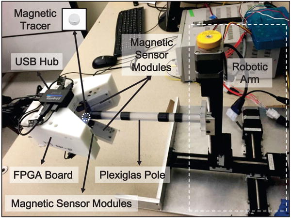
Experimental setup for magnetic calibration and localization.

The rest of the paper is organized as follows. Section II introduces the architecture of TTS. Section III first describes the probabilistic model for magnetic measurement and tracer state, then provides the joint calibration and localization (JCL) algorithm based on EM. Section IV presents the experimental results and discussion followed by conclusions in section V. The notations used in this paper are list as follows: Upper (lower) bold face letters are used for matrices (column vectors). (·)^T denotes transposition. E(·) refers the expectation. I_n is an identity matrix of size n. cov(·) denotes the covariance function. |A| denotes the determinant of matrix A. tr(A) denotes the trace of matrix A. δ(·,·) refers to the Kronecker Delta function. ⊙ denotes dot product.

II. Tongue tracking system overview

The experimental setup for magnetic calibration and localization is shown in Fig. 1, including a magnetic tracer, a robotic arm with non-magnetic Plexiglas pole, an array of 24 magnetic sensor modules, a field programmable gate array (FPGA) board housed in the white 3-D printed enclosure, and a USB hub. The tracer, i.e., a small disc-shaped permanent magnet (diameter: 6.05 mm, thickness: 1.25 mm, weight: 0.09 g, residual induction: 14800 G) (KJ Magnetics, Jamison, PA), was mounted on the end of the Plexiglas pole (25 cm) and positioned by the 3-D robotic arm (VELMEX, Bloomfield, NY) with a 3.75 μm spatial resolution. The 3-axial magnetic sensors (LSM303, STMicroelectronics, Perinton, NY) were grouped in six modules of 4 sensors each, and delivered the digitized measured magnetic field to a PC via USB port for tracer localization. The positioning of the sensor modules is aimed at capturing the changes in magnetic field due to tongue motion, by surrounding the cheek and jaw when patients use this system for tongue tracking. Each sensor module accommodated four sensor chips, which included an amplifier, a 12-bit ADC, and an I2C serial interface. The data from all sensors were collected at 100 Hz sampling rate by the FPGA (Mojo Board V3, Embedded Micro, Mountain View, CA), which includes a Spartan 6 XC6SLX9 FPGA via SPI communication interface, where the data were packetized and sent to a Windows PC, which was connected to the Mojo board by a USB cable. A custom graphical user interface (GUI) was developed in Windows environment to collect and store data from USB port, and to visualize the magnetic sensors signals in real time. In addition, a software developed by TinyG was implemented to control the robotic arm. To calibrate the gain and offset of each sensor, and indicate its 3-D position and orientation, with respect to the system origin and coordinates, a 3-D trajectory was programmed in the TinyG software. The robotic arm with the magnetic tracer mounted on the Plexiglas pole was moved according to the trajectory presented in the software. After calibration, the evaluation dataset for localization was collected in a similar way but with a different trajectory, to evaluate the tracking accuracy.

III. Methods

A. Model of Magnetic Measurements and Tracer Motions

Fig. 2 shows a cylindrical magnetic tracer with thickness l and diameter d, at location p = [p_x, p_y, p_z]^T. The orientation of the dipole moment, m, is determined by θ and ϕ. The static magnetic flux density, f, generated by this magnet, measured at the sensor location s = [s_x, s_y, s_z]^T, at a distance much greater than l and d, fits the magnetic dipole model, described by the Euler’s equation as follows [12]:

$$\mathbf{f}(\mathbf{s},\mathbf{p},\mathbf{m})=\frac{{\mu }_0}{4\pi }\frac{3{\mathbf{m}}^T(\mathbf{s}-\mathbf{p})(\mathbf{s}-\mathbf{p})-{\Vert \mathbf{s}-\mathbf{p}\Vert }^2\mathbf{m}}{{\Vert \mathbf{s}-\mathbf{p}\Vert }^5},$$ (1)

where m = [m sin θ cos ϕ, m sin θ sin ϕ, m cos θ]^T, with magnitude m = π f_rd²l/4μ₀, and f_r is the residual magnetic strength [10]. Given magnetic field data, f, and sensor position, s, the purpose of magnetic localization is to solve the unknown dipole variables including the position p and orientation, θ and ϕ. This is also known as solving the inverse problem [30]. (1) is valid only under ideal conditions, however, in practice, the measured magnetic field also depends on the the parameters of sensors (e.g., the gains, positions, orientations and offsets), and the ambient interferences (e.g., the EMF, residual magnetization in the nearby ferromagnetic objects, and induced field from electric current around the sensor). Therefore, we modify model (1) to express the magnetic field measured by a sensor, y, as follows:

$$\{\begin{array}{ll}\mathbf{y}=h(\mathbf{x},\psi )+\mathbf{v}\hfill & (2\mathrm{a})\hfill \\ h(\mathbf{x},\psi )=\mathbf{G}·\mathbf{H}·\mathbf{f}(\mathbf{s},\mathbf{p},\mathbf{m})+\mathbf{o}+{\mathbf{f}}_e\hfill & (2\mathrm{b})\hfill \end{array}$$

where h(·) is the modified function of dipole magnetic field, f_e denotes the earth’s magnetic field (EMF), v is the additive noise, dipole variable x = [p_x, p_y, p_z, θ, ϕ]^T, measurement parameters ψ = {G, H, s, o, f_e}, diagonal matrix G∈R^3×3 and vector o∈R³ are the gain and offset of the sensor, respectively; H represents the 3-D rotation matrix to correct the misalignment errors of individual sensor orientations, H^TH = I₃ and |H| = 1. In [9], we moved the tracer along a precise trajectory using a robotic arm, while simultaneously recording magnetic field data (i.e., given a group of x and y), then calibrated sensor parameters ψ, by resolving a nonlinear least square problem towards minimizing the variance of noise v. This calibration is data driven, i.e., with different sets of x and y, the optimized ψ may be different. Even if we collect plenty of x and y data to cover the spans of dipole variables and the corresponding magnetic field, the distributions of trajectories in calibration and evaluation are likely to be different, and the calibrated parameters are going to be biased as a result. This bias degrades the localization accuracy. Moreover, the measurement model expressed by (2) is static, and ignores the state transition of tracer, which reflects the tongue motion information. Therefore, we build a dynamic tracking model based on a stochastic system as follows:

$$\{\begin{array}{ll}{\mathbf{x}}_t={\mathbf{x}}_{t-1}+{\mathbf{w}}_{t-1}\hfill & (3\mathrm{a})\hfill \\ {\mathbf{y}}_t^j=h({\mathbf{x}}_t,{\psi }^j)+{\mathbf{v}}_t^j\hfill & (3\mathrm{b})\hfill \end{array}$$

where the state vector x_t∈R⁵ represents the position and angles of the magnetic dipole at time t, t = 1, 2, 3, …, T, with an initial distribution ${\mathbf{x}}_0\sim \mathcal{N}({\mathbf{m}}_0,{\mathbf{P}}_0)$, process noise ${\mathbf{w}}_{t-1}\sim \mathcal{N}(\mathbf{0},\mathbf{Q})$. Considering the close relationship between adjacent states during continuous movements, we assume x follows a first-order Markov process. The observation vector ${\mathbf{y}}_t^j\in R^3$ represents the magnetic field data measured by sensor j, j = 1, 2, 3, …, C, where C is the total number of sensors, observation noise ${\mathbf{v}}_t^j\sim \mathcal{N}(\mathbf{0},{\mathbf{R}}^j)$. Here we assume Q is diagonal, i.e., the components of tongue movements are unrelated with each other; assume R^j is diagonal and cov(v^j, vⁱ) = R^j ⊙ δ(i, j), i.e., the noise components of different sensors and axes are unrelated to each other. By combining all the sensors, (3b) can be written as

$${\mathbf{y}}_t=\hslash \left({\mathbf{x}}_t,({\psi }^1,\dots ,{\psi }^C)\right)+{\mathbf{v}}_t,$$ (4)

where ${\mathbf{y}}_t=[{\mathbf{y}}_t^1;\dots ;{\mathbf{y}}_t^C]$, ħ(x_t) = [h(x_t, ψ¹); …; h(x_t, ψ^C)], ${\mathbf{v}}_t~\mathcal{N}(\mathbf{0},\mathbf{R})$, R consists of R^j. In this dynamic tracking model, the distributions of state sequence {m_t, P_t}_t=0:T, the noise covariances {Q, R} and the sensor parameters {G^j, H^j, s^j, b^j}_j=1:C are estimated based on the measurements {y}_t=1:T, where ${\mathbf{b}}^j={\mathbf{o}}^j+{\mathbf{f}}_e^j$ is the general offset. The EMF, f_e, is assumed to be constant during the experiment, since the current TTS prototype, shown in Fig. 1, is stationary.

Fig. 2.

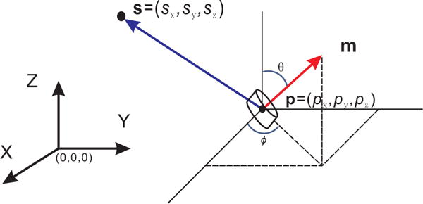
Vector representation of the magnetic dipole model [10].

B. Joint Calibration and Localization based on EM

For nonlinear dynamic systems, three kinds of approaches are usually used to estimate the states and parameters. First, the states are augmented with the parameters and recursively estimated by filtering methods [31]. However, this approach will result in large parameter covariance [32], and may cause the filter to diverge since the Gaussian approximation tends to become singular [33]. Second, the marginal likelihood of the parameters is directly approximated by filtering methods, then parameters are sought by numerical optimization [34]. This approach needs more complex derivations and cannot easily address the orthogonal constraints on sensor rotation matrix for our application. The third is EM algorithm [27] which iteratively optimizes the parameters to maximize the lower bound of log-likelihood of measurements. EM works efficiently when the parameter optimization is performed in closed-form. In the proposed tracking model, the sensor positions, s, are involved in the nonlinear dipole equation, have no closed-form solution. Considering the inaccuracies involved in the 3-D printing and installation of TTS components and sensors during system assembly, s was known with a range of uncertainty within ±3mm. Here s was identified only once with a known trajectory and was not included in the subsequent alternative calibration and localization steps. The sensor rotation matrix H with orthogonal constraints has no closed-form solution either. Here, we present two strategies: first, calibrating H once with a known trajectory, only adjusting G, b, Q, and R analytically in EM; second, optimizing H with these parameters by embedding a curvilinear search algorithm [29] in EM. The performances of these two strategies are compared in section IV. Here we describe EM algorithm for the tongue tracking application as follows.

EM is an iterative algorithm for seeking maximum likelihood parameter estimates when the model depends on latent variables. For our case, we estimate sensor parameters and noise variances, based on the observed magnetic field y_1:T. The latent variables are the sequence of dipole positions and orientations, x_1:T. EM algorithm iteratively performs expectation (E) step and maximum (M) step until it convergences. E step uses y_1:T and current parameter estimates Θ^(k) to infer the latent variables x_1:T, then computes the conditional expectation of likelihood; The M step updates the parameter estimates by maximizing the expectation. The above processing steps can be formulated as

$${\mathbf{\Theta }}^{k+1}={\text{argmax}}_{\mathbf{\Theta }}\mathrm{E}[\mathit{log}(L)|{\mathbf{y}}_{1:T},{\mathbf{\Theta }}^{(k)}],$$ (5)

where L = p(y_1:T, x_1:T|Θ) is the likelihood function with respect to Θ. Based on the first-order Markov process, L can be expressed as

$$L=p({\mathbf{x}}_0|\mathbf{\Theta }){\displaystyle \prod _{t=1}^{T}p({\mathbf{x}}_t|{\mathbf{x}}_{t-1},\mathbf{\Theta })}{\displaystyle \prod _{t=1}^{T}p({\mathbf{y}}_t|{\mathbf{x}}_t,\mathbf{\Theta })}.$$ (6)

a) E Step

The computation of E[log(L)|y_1:T, Θ^(k)] requires the knowledge of smoothing distributions p(x_t|y_1:T Θ^(k)) and p(x_t, x_t−1|y_1:T, Θ^(k)) [33]. For nonlinear models, they are estimated by Gaussian smoother approximation methods, such as extended Rauch-Tung-Striebel smoother (ERTSS) with Taylor series approximations [35] and URTSS [28] with unscented transform. The unscented transform deterministically chooses sigma points to capture the mean and covariance of a random variable undergoing a nonlinear transformation, does not need to compute the Jacobians, and is more accurate than Taylor series approximations [36]. Therefore, we employ URTSS to estimate the smoothing distributions as follows [33]:

$$\{\begin{array}{ll}\begin{array}{l}p({\mathbf{x}}_t|{\mathbf{y}}_{1:T},{\mathbf{\Theta }}^{(k)})\approx \mathcal{N}({\mathbf{x}}_t|{\mathbf{m}}_t^s,{\mathbf{P}}_t^s)\\ p({\mathbf{x}}_t,{\mathbf{x}}_{t-1}|{\mathbf{y}}_{1:T},{\mathbf{\Theta }}^{(k)})\end{array}\hfill & (7\mathrm{a})\hfill \\ \approx \mathcal{N}\left(\left[\begin{array}{c}{\mathbf{x}}_t\\ {\mathbf{x}}_{t-1}\end{array}\right]|\left[\begin{array}{c}{\mathbf{m}}_t^s\\ {\mathbf{m}}_{t-1}^s\end{array}\right],\left[\begin{array}{cc}{\mathbf{P}}_t^s& {\mathbf{P}}_t^s{\mathbf{K}}_{t-1}^T\\ {\mathbf{K}}_{t-1}{\mathbf{P}}_t^s& {\mathbf{P}}_{t-1}^s\end{array}\right]\right)\hfill & (7\mathrm{b})\hfill \end{array}$$

where ${\{{\mathbf{m}}_t^s,{\mathbf{P}}_t^s\}}_{t=1:T}$ are the means and covariances estimated by URTSS, K_t−1 is the smoother gain. Then the conditional expectation of likelihood is computed as follows [34]:

$$\mathrm{E}[\mathit{log}(L)|{\mathbf{y}}_{1:T},{\mathbf{\Theta }}^{(k)}]\approx -\frac{1}{2}\mathit{log}|2\pi {\mathbf{P}}_0|-\frac{T}{2}\mathit{log}|2\pi \mathbf{Q}|-\frac{T}{2}\mathit{log}|2\pi \mathbf{R}|-\frac{1}{2}tr\{{\mathbf{P}}_0^{-1}[{\mathbf{P}}_0^s+({\mathbf{m}}_0^s-{\mathbf{m}}_0){({\mathbf{m}}_0^s-{\mathbf{m}}_0)}^T]\}-\frac{1}{2}{\displaystyle \sum _{t}tr\{{\mathbf{Q}}^{-1}\mathrm{E}[({\mathbf{x}}_t-{\mathbf{x}}_{t-1}){({\mathbf{x}}_t-{\mathbf{x}}_{t-1})}^T|{\mathbf{y}}_{1:T}]\}}-\frac{1}{2}{\displaystyle \sum _{t}tr\{{\mathbf{R}}^{-1}\mathrm{E}{[{\mathbf{y}}_t-\hslash ({\mathbf{x}}_t)]}^T{[{\mathbf{y}}_t-\hslash ({\mathbf{x}}_t)]}^T|{\mathbf{y}}_{1:T}]\}},$$ (8)

$$\mathrm{E}[({\mathbf{x}}_t-{\mathbf{x}}_{t-1}){({\mathbf{x}}_t-{\mathbf{x}}_{t-1})}^T|{\mathbf{y}}_{1:T}]\approx {\mathbf{P}}_t^s+{\mathbf{m}}_t^s{[{\mathbf{m}}_t^s]}^T+{\mathbf{P}}_{t-1}^s+{\mathbf{m}}_{t-1}^s{[{\mathbf{m}}_{t-1}^s]}^T{\mathbf{P}}_t^s{\mathbf{K}}_{t-1}^T-{\mathbf{m}}_t^s{[{\mathbf{m}}_{t-1}^s]}^T-{\mathbf{K}}_{t-1}{\mathbf{P}}_t^s-{\mathbf{m}}_{t-1}^s{[{\mathbf{m}}_t^s]}^T,$$ (9)

$$\mathrm{E}\{[{\mathbf{y}}_t-\hslash ({\mathbf{x}}_t)]{[{\mathbf{y}}_t-\hslash ({\mathbf{x}}_t)]}^T|{\mathbf{y}}_{1:T}\}\approx {\mathbf{y}}_t{\mathbf{y}}_t^T-{\mathbf{y}}_t{\displaystyle \sum _t{\omega }_i^{(m)}\hslash {({\mathbf{\chi }}_{t,i})}^T}-{\displaystyle \sum _i{\omega }_i^{(m)}\hslash ({\mathbf{\chi }}_{t,i}){\mathbf{y}}_t^T+{\displaystyle \sum _i{\omega }_i^{(c)}}}·\hslash ({\mathbf{\chi }}_{t,i})\hslash {({\mathbf{\chi }}_{t,i})}^T,$$ (10)

where χ_t,i, i = 0, 1, 2, …, 2n are the sigma points sampled from smoothing distribution $\{{\mathbf{m}}_t^s,{\mathbf{P}}_t^s\}$, ${\omega }_i^{(m)}$ and ${\omega }_i^{(c)}$ are the associated weights for the mean estimates and covariance estimates propagated through nonlinear function ħ(·), respectively. They are computed as follows [36]:

$$\{\begin{array}{ll}{\mathbf{\chi }}_{t,0}={\mathbf{m}}_t^s\hfill & (11\mathrm{a})\hfill \\ {\mathbf{\chi }}_{t,i}={\mathbf{m}}_t^s+{\left(\sqrt{(n+\mathrm{\lambda }){\mathbf{P}}_t^s}\right)}_i,i=1,\dots ,n.\hfill & (11\mathrm{b})\hfill \\ {\mathbf{\chi }}_{t,i}={\mathbf{m}}_t^s-{\left(\sqrt{(n+\mathrm{\lambda }){\mathbf{P}}_t^s}\right)}_{i-n},i=n+1,\dots ,2n.\hfill & (11\mathrm{c})\hfill \\ {\omega }_0^{(m)}=\mathrm{\lambda }/(n+\mathrm{\lambda })\hfill & (11\mathrm{d})\hfill \\ {\omega }_0^{(c)}=\mathrm{\lambda }/(n+\mathrm{\lambda })+(1-{\alpha }^2+\beta )\hfill & (11\mathrm{e})\hfill \\ {\omega }_i^{(m)}={\omega }_i^{(c)}=1/\{2(n+\mathrm{\lambda })\},i=1,\dots ,2n.\hfill & (11\mathrm{f})\hfill \\ \mathrm{\lambda }={\alpha }^2(k+\kappa )-n\hfill & (11\mathrm{g})\hfill \end{array}$$

where ${\left(\sqrt{(n+\mathrm{\lambda }){\mathbf{P}}_t^s}\right)}_i$ is the ith column of the matrix square root. Here we use a common setting α = 1, β = 0, κ = 0 [34], then ${\omega }_0^{(c)}={\omega }_0^{(m)}=0$, and (9) can be simplified as

$$\mathrm{E}\{[{\mathbf{y}}_t-\hslash ({\mathbf{x}}_t)]{[{\mathbf{y}}_t-\hslash ({\mathbf{x}}_t)]}^T|{\mathbf{y}}_{1:T}\}\approx \frac{1}{2n}{\displaystyle \sum _{i=1}^{2n}[{\mathbf{y}}_t-\hslash ({\mathbf{\chi }}_{t,i})]{[{\mathbf{y}}_t-\hslash ({\mathbf{\chi }}_{t,i})]}^T}.$$ (12)

b) M Step

Setting the partial derivatives with respect to Q, R, P₀ and m₀ equal to zeros, it is easy to compute the optimal parameters $\widehat{\mathbf{Q}}$, $\widehat{\mathbf{R}}$, ${\widehat{\mathbf{P}}}_0$ and ${\widehat{\mathbf{m}}}_0$ for maximizing E[log(L)|y_1:T, Θ^(k)] at the kth iteration as follows [34]:

$$\{\begin{array}{ll}\widehat{\mathbf{Q}}=\frac{1}{T}{\displaystyle \sum _t\mathrm{E}\left[\left({\mathbf{x}}_t-{\mathbf{x}}_{t-1}\right){\left({\mathbf{x}}_t-{\mathbf{x}}_{t-1}\right)}^T|{\mathbf{y}}_{1:T}\right]}\hfill & \left(13\mathrm{a}\right)\hfill \\ \widehat{\mathbf{R}}=\frac{1}{T}{\displaystyle \sum _t\mathrm{E}\left[\left({\mathbf{y}}_t-\hslash \left({\mathbf{x}}_t\right)\right){\left({\mathbf{y}}_t-\hslash \left({\mathbf{x}}_t\right)\right)}^T|{\mathbf{y}}_{1:T}\right]}\hfill & \left(13\mathrm{b}\right)\hfill \\ {\widehat{\mathbf{P}}}_0={\mathbf{P}}_0^s+\left({\mathbf{m}}_0^s-{\mathbf{m}}_0\right){\left({\mathbf{m}}_0^s-{\mathbf{m}}_0\right)}^T\hfill & \left(13\mathrm{c}\right)\hfill \\ {\widehat{\mathbf{m}}}_0={\mathbf{m}}_0^s\hfill & \left(13\mathrm{d}\right)\hfill \end{array}$$

Based on (8) and (12), the optimization of G, H, and b can be approximated by resolving a least square problem as

$$minJ\left(\mathbf{G},\mathbf{H},\mathbf{b}\right)=tr\left\{{\mathbf{R}}^{-1}{\displaystyle \sum _{t,i}\left[{\mathbf{y}}_t-\hslash \left({\mathbf{\chi }}_{t,i}\right)\right]}{\left[{\mathbf{y}}_t-\hslash \left({\mathbf{\chi }}_{t,i}\right)\right]}^T\right\}.$$ (14)

Denoting $r_k^j={[{\mathbf{R}}^j(k,k)]}^{-1/2}$ and ${\mathbf{z}}_{t,i}=\left[r_k^j{\mathbf{H}}_k^j\mathbf{f}\left({\mathbf{\chi }}_{t,i},{\mathbf{s}}^j\right),r_k^j\right]$, according to the magnetic measurement equations (2b) and (4), the closed-form solutions of G and b for each sensor are given as follows:

$$\left[{\mathbf{G}}^j\left(k,k\right),{\mathbf{b}}^j\left(k\right)\right]=\left[{\displaystyle \sum _{t,i}{r}_k^j{\mathbf{y}}_t^j\left(k\right){\mathbf{z}}_{t,i}}\right]{\left[{\displaystyle \sum _{t,i}{\mathbf{z}}_{t,i}^T{\mathbf{z}}_{t,i}}\right]}^{-1}$$ (15)

where j is the sensor number, ${\mathbf{H}}_k^j$ is the kth row of H^j, and k = 1, 2, 3 are responding to the three axes. Denoting ${\mathbf{a}}_t^j={\left({\mathbf{R}}^j\right)}^{-1/2}\left({\mathbf{y}}_t^j-{\mathbf{b}}^j\right)$ and B^j = (R^j)^−1/2G^j, then the optimization of H^j can be expressed by resolving a weighted orthogonal Procrustes problem as follows:

$$\{\begin{array}{ll}minJ\left({\mathbf{H}}^j\right)={\displaystyle \sum _{t,i}{\Vert {\mathbf{a}}_t^j-{\mathbf{B}}^j{\mathbf{H}}^j\mathbf{f}\left({\mathbf{\chi }}_{t,i},{\mathbf{s}}^j\right)\Vert }_2^2}\hfill & \left(16\mathrm{a}\right)\hfill \\ s.t.{\left({\mathbf{H}}^j\right)}^T{\mathbf{H}}^j={\mathbf{I}}_3,\left|\mathbf{H}\right|=1.\hfill & \left(16\mathrm{b}\right)\hfill \end{array}$$

Denoting ${\mathbf{A}}^j=\left[{\mathbf{a}}_1^j{\mathbf{1}}_{2n}^T,\dots ,{\mathbf{a}}_t^j{\mathbf{1}}_{2n}^T,\dots ,{\mathbf{a}}_T^j{\mathbf{1}}_{2n}^T\right]$, ${\mathbf{C}}^j=\left[{\mathbf{F}}_1^j,\dots ,,{\mathbf{F}}_t^j,\dots ,{\mathbf{F}}_T^j\right]$ and ${\mathbf{F}}_t^j=\left[\mathbf{f}\left({\mathbf{\chi }}_{t,1},{\mathbf{s}}^j\right),\dots ,\mathbf{f}\left({\mathbf{\chi }}_{t,2n},{\mathbf{s}}^j\right)\right]$, then (16) can be rewritten in matrix form as follows:

$$\{\begin{array}{ll}minJ\left({\mathbf{H}}^j\right)={\Vert {\mathbf{A}}^j-{\mathbf{B}}^j{\mathbf{H}}^j{\mathbf{C}}^j\Vert }_F^2\hfill & \left(17\mathrm{a}\right)\hfill \\ s.t.{\left({\mathbf{H}}^j\right)}^T{\mathbf{H}}^j={\mathbf{I}}_3,\left|\mathbf{H}\right|=1.\hfill & \left(17\mathrm{b}\right)\hfill \end{array}$$

This problem does not have a closed-form solution, but can be solved by iterative methods, which generate a sequence of feasible points converging to a local minima. These iterative methods are often computationally expensive in order to preserve the orthogonal constraint, such as using singular value decomposition [37], or searching along geodesic by solving partial differential equations [38]. To reduce the computation time, a curvilinear search algorithm based on the Cayley transform has been developed recently [29], which is briefly described as below. Given feasible point H and gradient $\mathbf{U}=\frac{\partial J}{\partial \mathbf{H}}$, then a skew-symmetric matrix W is defined as W : UH^T − HU^T. According to the Cayley transform [39], ${\left(\mathbf{I}+\frac{\tau }{2}\mathbf{W}\right)}^{-1}\left(\mathbf{I}-\frac{\tau }{2}\mathbf{W}\right)$ is a rotation matrix. Then the new trial point is computed by

$$\overline{\mathbf{H}}={\left(\mathbf{I}+\frac{\tau }{2}\mathbf{W}\right)}^{-1}\left(\mathbf{I}-\frac{\tau }{2}\mathbf{W}\right)\mathbf{H},$$ (18)

where the step size τ can be estimated by Barzilai-Borwein method [40]. And the non-monotone strategy [41] is used to guarantee global convergence. To apply the curvilinear search in our case, we compute the gradient U according to (17a) as follows (the superscript j is not shown for simplicity):

$$J\left(\mathbf{H}\right)=tr\left[{\left(\mathbf{A}-\mathbf{BHC}\right)}^T\left(\mathbf{A}-\mathbf{BHC}\right)\right]=tr\left({\mathbf{A}}^T\mathbf{A}\right)-2tr\left[{\left(\mathbf{HC}\right)}^T{\mathbf{B}}^T\mathbf{A}\right]+tr\left[{\left(\mathbf{HC}\right)}^T{\mathbf{B}}^T\mathbf{B}\left(\mathbf{HC}\right)\right],$$ (19)

$$\frac{\partial J}{\partial \mathbf{H}}=-2{\mathbf{B}}^T\mathbf{A}{\mathbf{C}}^T+2{\mathbf{B}}^T\mathbf{B}\left(\mathbf{HC}\right){\mathbf{C}}^T=2{\mathbf{B}}^T\left(\mathbf{BHC}-\mathbf{A}\right){\mathbf{C}}^T.$$ (20)

The procedure of joint magnetic calibration and localization is summarized in Algorithm 1. H_f controls the optimization of sensor rotation matrix H. At step 14, setting break means running JCL without updating H (JCLNSR); instead, setting H_f = 1 means further running JCL with the update of H after JCLNSR convergences. The initial sensor parameters ${\mathbf{\Omega }}_s^0$ were estimated by our previous method [9] using a calibration data set with known trajectory and recorded magnetic field data. The sensor positions s were not updated during the EM optimization. In calibration data set we estimated the sensor offsets o⁰, while for evaluation we remeasured the EMF, and generate initial general offset b⁰ = o⁰ + f_e. The mean of prior distribution ${\mathbf{m}}_0^0$ was estimated by computing the first point of trajectory with the method proposed in [18]. The initial covariances ${\mathbf{P}}_0^0$ and ${\mathbf{\Omega }}_c^0$ were set empirically.

Algorithm 1.

Joint magnetic calibration and localization

Input: The number of iterations L, the stop threshold δ of EM algorithm, the recorded magnetic field data Y = {y}t=1:T, initial sensor parameters ${\mathbf{\Omega }}_s^0=\{{\mathbf{G}}^0,{\mathbf{b}}^0,{\mathbf{H}}^0,\mathbf{s}\}$, initial prior distribution ${\mathbf{\Omega }}_p^0=\left\{{\mathbf{m}}_0^0,{\mathbf{P}}_0^0\right\}$ and initial noise covariances ${\mathbf{\Omega }}_c^0=\left\{{\mathbf{Q}}^0,{\mathbf{R}}^0\right\}$. Hf = 0.
1:	for n = 1 : L do
2:	Run URTSS with Y and $\left\{{\mathbf{\Omega }}_s^{n-1},{\mathbf{\Omega }}_p^{n-1},{\mathbf{\Omega }}_c^{n-1}\right\}$ to estimate ${\mathbf{X}}^{n-1}={\left\{{\mathbf{m}}_t^s,{\mathbf{P}}_t^s\right\}}_{t=1:T}^{n-1}$;
3:	Update $\left\{{\mathbf{\Omega }}_p^{n-1},{\mathbf{\Omega }}_c^{n-1}\right\}$ to $\left\{{\mathbf{\Omega }}_p^n,{\mathbf{\Omega }}_c^n\right\}$ with respect to ${\mathbf{\Omega }}_s^{n-1}$, Y and Xn−1 according to (9)–(13);
4:	if Hf = 0 then
5:	Update ${\mathbf{\Omega }}_s^{n-1}$ to ${\mathbf{\Omega }}_s^n$ by computing {Gn, bn} with respect to Rn, Hn−1, Y and Xn−1 according to (15);
6:	else
7:	Update ${\mathbf{\Omega }}_s^{n-1}$ to ${\mathbf{\Omega }}_s^n$ by alternately optimizing {G, b} and H based on curvilinear search according to (15), (17), (18) and (20).
8:	end if
9:	Compute the J(n) = [E(log(L)]n with respect to $\left\{{\mathbf{\Omega }}_s^n,{\mathbf{\Omega }}_p^n,{\mathbf{\Omega }}_c^n\right\}$, Y and Xn−1 according to (8);
10:	if n > 1, Hf = 1 and $\left|\frac{J(n)-J(n-1)}{J(n-1)}\right|<\delta$ then
11:	break, end;
12:	end if
13:	if n > 1, Hf = 0 and $\left|\frac{J(n)-J(n-1)}{J(n-1)}\right|<\delta$ then
14:	break or Hf = 1 (optional), end;
15:	end if
16:	end for
Output: The optimized {Ωs, Ωp, Ωc} and X.

IV. Evaluation

In this section, we present experimental data to show the bias of separate calibration across different datasets, and assess the performance of the proposed JCL algorithm in reducing calibration bias and improving localization accuracy.

A. Data Sets

We placed the magnetic tracer on the tip of the robotic arm in different orientations, and controlled the robotic arm to move along different trajectories, as shown in Fig. 3. At the same time, the magnetic field data were recorded by the 24 three-axial sensors. Based on different combinations of orientations and trajectories, fifteen datasets were generated, as listed in Table I. The average speed of the robotic arm movement has a mean of 8.29 mm/s and standard deviation of 0.26 mm/s. In order to emulate various tongue movement speeds, we have down-sampled the trajectories and looked at the effect on the localization. After down-sampling, the speed of movement reach mean of 131 mm/s and standard deviation of 130 mm/s, which are closer to the maximum speed of the tongue motion. The experiments were performed at the same location in different days within a month.

Fig. 3.

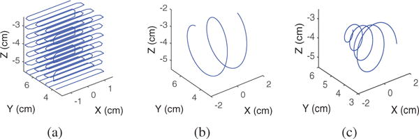
Different target trajectories in the 3 × 3 × 3 cm³ experimental space. (a) cube: 537 sample points; (b) Helix: 455 sample points; (c) Fermats spiral: 553 sample points.

Table I.

Data Sets D1–D15 with Different Tracer Trajectories and Orientations (Varying in Angle θ, While Keeping Angle ϕ = 0° Degree for All the Datasets)

Traj.	θ = 0°	θ = −45°	θ = 45°	θ = −135°	θ = 135°
Cube	D1	D2	D3*	D4*	D5*
Helix	D6	D7	D8	D9	D10
Spiral	D11	D12	D13	D14	D15

^*D3: θ = 35°, D4: θ = −130°, D5: θ = 125°.

B. Diversity of Calibration Result on Different Data Sets

We calibrated the sensor parameters based on the nonlinear least square method in [9] using data sets D1–D15. The 24 three-axial sensors are considered as 72 individual channels. The gains of sensors G are arranged as a vector, {[g_x(1), g_y(1), g_z(1)], [g_x(2), g_y(2), g_z(2)]}, ⋯, [g_x(24), g_y(24), g_z(24)]} ∈ R⁷². The sensor Euler angles for misalignment error are transformed from the three-dimensional rotation matrix H using the method in [42] and arranged as a vector {[e_x(1), e_y(1), e_z(1)], [e_x(2), e_y(2), e_z(2)], ⋯, [e_x(24), e_y(24), e_z(24)]} ∈ R⁷². The positions and offsets of sensors are represented in a similar way. Figs. 4a–4d use box plots to show the distributions of the estimated sensor parameters across datasets for each of the 72 channels. The spacing between the top and bottom of each box indicates the degree of dispersions in the estimated parameters. Figs. 4a and 4b show that the dispersions in sensor gains and offsets for most channels are clear, which reveal the biases of calibration across different datasets; while Figs. 4c and 4d show that the dispersions in sensor angles and positions are small, which means they are not sensitive to different datasets. Therefore, considering the trade-off between calibration accuracy and computation efficiency, as mentioned in Section II.B, the proposed JCL algorithm iteratively updates the estimation of sensor gains and offsets, sets the update of sensor rotation matrix H as an option, but does not update the estimation for sensor positions.

Fig. 4.

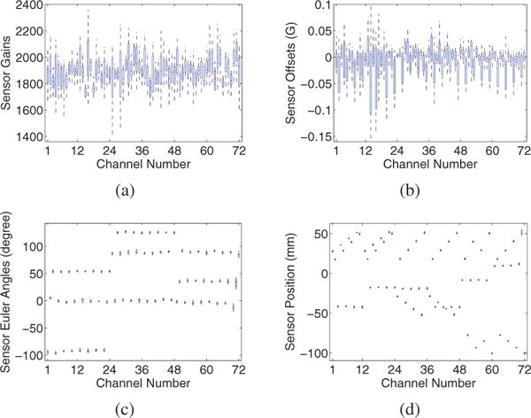
Distributions of the estimated sensor parameters: (a) gains, (b) offsets, (c) Euler angles, (d) positions, across 15 data sets for each of the 72 channels. The middle line, the bottom, and the top of the box represent the median, the 25th, and the 75th percentiles, respectively. The whiskers represent the furthermost value in the 1.5 interquartile ranges. Outliers are not represented in this figure.

C. Convergence of the JCL algorithm

Using D1 (cube trajectory, θ = 0°) as the calibration data set, and D2–D15 as the evaluation data sets, we tested the JCL algorithm with and without the update of sensor rotation matrix, denoted by JCL and JCLNSR, respectively. We observed the numbers of iterations they took before the stop criterion were met, i.e. |[J(n)− J(n−1)]/J(n−1)| < 10⁻³, where J is the conditional expectation of log-likelihood (CEL) estimated by (8), and n is the iteration number. Based on (6), we know that the likelihood function L ≤ 1, and then CEL J ≤ 0. Fig. 5a shows the CELs calculated by JCLNSR over iterations for all the evaluation data sets, which increased markedly in the early iterations and rapidly converged to a stable negative value. This result demonstrates the climbing hill optimization of JCLNSR and coincides with the derivation of (6) that CEL J ≤ 0. Across all 14 evaluation datasets, the JCLNSR algorithm took 4 – 17 iterations to meet the stop criterion, with a mean of 9.71 and a standard deviation of 4.10 iterations. Fig. 5b shows the CELs calculated by JCL. It is clear that after JCLNSR converged, the sensor rotation matrix H was involved in the alternative update of JCL, then the CELs further increased a few steps and converged again. That suggests the updates of H improve the fitting of measured magnetic field with our probability model. The proposed algorithms were implemented in Matlab and C mixed programming. The computations were run on Windows 7 Professional SP1 64 bit with Intel Core CPU i7-6700K @ 4.00 GHz. The time for JCLNSR for each dataset ranged between 0.58 and 1.96 minutes. The time for JCL for each dataset ranged between 2.02 and 4.91 minutes. However, once the sensors and noise parameters are calibrated, the localization time of unscented Kalman filtering for each data point is within 10 ms. That indicates we can run JCLNSR/JCL in the background or at the rest intervals between sessions to update the parameters in batch mode, and perform tongue tracking during sessions.

Fig. 5.

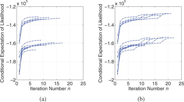
Conditional expectations of likelihood calculated by (a) JCLNSR and (b) JCL, over the number of iterations.

D. Comparison of Calibration Performance

The calibration biases of the JCL algorithm and the nonlinear least square method in [9] are listed in Table II. The sensor parameters directly computed on each evaluation data set with known trajectories and magnetic tracer orientations are considered as the target values x^∗ ∈ R⁷² (for 72 channels). The normalized calibration bias is computed as ‖x−x^∗‖/‖x^∗‖, where x is the estimated value without known trajectories and magnetic tracer orientations in evaluation datasets. On average, the estimation biases of JCL are smaller than those of our previous algorithm for all the sensor parameters. The superiority of JCL on the estimation of sensor offsets is significant (paired t-test, p = 2.55 × 10⁻⁴). This is because JCL takes advantage of sensor measurements in evaluation datasets and uses the knowledge of continuous movements of magnetic tracer, to adaptively adjust the estimation of parameters, while our previous algorithm only depends on the information from calibration data set D1.

Table II.

Estimation Biases (%) of Sensor Parameters with the Seperate Calibration Algorithm (S) [9] and with the JCL (J). The Lowest Bias for Each Dataset and Parameter Is in Bold Italic.

Evaluation	Gain		Euler Angle		Offset
Datasets	S	J	S	J	S	J
D2	4.37	3.50	2.62	2.72	328.53	69.66
D3	10.18	7.90	2.55	2.40	28.87	21.69
D4	8.32	6.81	2.90	2.80	67.04	30.63
D5	5.54	2.38	1.87	1.48	40.23	15.48
D6	6.20	6.40	4.09	4.03	128.20	34.12
D7	13.99	9.24	4.17	4.01	189.03	83.21
D8	7.98	5.74	3.56	3.63	147.61	35.41
D9	10.64	6.31	3.56	3.44	184.63	37.50
D10	13.65	13.20	4.60	4.43	289.97	113.99
D11	8.48	8.60	4.60	4.67	136.00	44.94
D12	14.72	11.18	4.39	4.34	171.58	99.19
D13	10.00	8.03	4.02	4.09	166.67	54.98
D14	11.69	6.15	4.49	4.30	197.67	63.12
D15	16.08	15.91	5.84	5.28	226.83	133.85
Avg.	10.13	7.95	3.81	3.69	164.49	59.84
Std.	3.58	3.60	1.04	1.02	85.24	36.05

E. Comparison of Localization Accuracy

Table III shows the RMSE obtained for each evaluation data set with different localization algorithms. LIN, LIN+LM and NM denotes linear algorithm, hybrid algorithm and nonlinear algorithm proposed in [13], [18] and [10], respectively. All of these three algorithms used the sensor parameters estimated from dataset D1, based on the nonlinear least square calibration method in [9]. On average, JCL achieved the best performance both in position (0.45 mm) and in orientation (2.33°). A one-way ANOVA with repeated measures indicated that the five algorithms differed significantly in both position and orientation (d.f. = 4, F = 32.81, p = 5.76 × 10⁻¹⁵ and d.f. = 4, F = 28.08, p = 1.48 × 10⁻¹³, respectively). Additional paired t-test showed that the JCL and JCLNSR were significantly better than each of the other algorithms in position (p ≤ 1.97 × 10⁻⁵). Furthermore, JCL significantly outperformed LIN, LIN+LM and NM in orientation (p ≤ 0.04).

Table III.

Comparing Localization Performances in Terms of RMSE in Tracer Position (P) and Orientation (O), Obtained for Each Evaluation Dataset with Different Algorithms. The Lowest RMSE for Each Dataset Is in Bold Italics.

Evaluation	LIN[13]		LIN+LM [18]		NM [10]		JCLNSR		JCL
Datasets	P(mm)	O(deg.)	P(mm)	O(deg.)	P(mm)	O(deg.)	P(mm)	O(deg.)	P(mm)	O(deg.)
D2	3.22	14.03	1.39	3.97	0.99	2.46	0.52	2.53	0.47	2.20
D3	1.24	3.86	0.54	1.40	0.52	1.19	0.39	0.66	0.39	0.65
D4	1.49	3.59	0.63	2.23	0.62	2.43	0.43	1.50	0.43	1.53
D5	1.60	3.63	0.51	1.30	0.51	1.21	0.39	1.41	0.40	1.60
D6	2.54	7.78	0.98	2.63	0.99	4.10	0.43	3.07	0.45	2.81
D7	2.21	9.79	1.61	4.63	1.20	3.93	0.68	3.38	0.63	3.39
D8	2.72	12.10	1.40	5.16	1.32	3.96	0.61	2.29	0.59	2.23
D9	4.48	15.55	1.23	4.72	0.95	3.96	0.62	2.70	0.53	2.73
D10	2.65	10.75	1.44	4.19	1.14	2.90	0.45	0.97	0.43	0.98
D11	1.52	6.41	0.62	3.35	0.57	4.40	0.27	3.66	0.28	3.49
D12	1.24	7.86	1.25	3.99	1.05	3.47	0.59	3.63	0.49	3.55
D13	1.62	11.75	1.07	5.69	0.89	4.31	0.50	4.05	0.44	3.70
D14	2.84	13.39	1.21	4.85	0.85	3.87	0.59	2.94	0.50	2.94
D15	1.51	9.28	1.04	4.16	0.75	2.92	0.30	0.97	0.29	0.81
Avg.	2.21	9.27	1.07	3.73	0.88	3.22	0.48	2.41	0.45	2.33
Std.	0.93	3.93	0.36	1.37	0.26	1.08	0.12	1.13	0.10	1.06

The relative poor performances of the LIN, LIN+LM and NM algorithms probably resulted from inter-dataset differences in observation noises and trajectories of the magnetic tracer, which caused error in calculating the magnetic field in ideal dipole model, expressed in (1), with the biased estimations of sensor parameters. Especially, LIN algorithm, which computes the inverse of matrix of magnetic field data [13], was very sensitive to this error, LIN+LM algorithm uses LIN for initial estimation of each sample, then performs fine gradient search, improves the localization performances, but still partially suffers from the drawback of LIN. The NM algorithm, which only employs LIN for the initialization of the first sample, then implicitly uses the state transition relationship of continuous magnet movements for localization of the following samples, was less influenced by the inter-dataset differences. The JCL algorithm employs a Bayesian framework and EM algorithm to correct the estimation of system parameters based on the magnetic sensor measurement in evaluation datasets and adapts to the inter-dataset differences. Fig. 6 shows the examples of localization results for different evaluation data sets. The trajectories reconstructed by JCL are clearly closer to the ground truth. The great average errors in orientation of all the methods (> 2°) are partly due to the manual setting errors of the angles θ and ϕ.

Fig. 6.

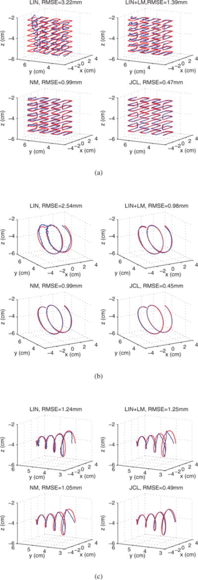
Examples of localization results obtained by different algorithms on: (a) data set D2, (b) data set D6, and (c) data set D12. The reconstructed trajectories are marked by blue dashed lines, and the ground truth trajectories are marked by red lines.

F. Data Requirement of JCL

In the tracking model of JCL (see (3)), we use the magnetic field data from evaluation sets to adjust the gain, offset, angles (i.e., rotation matrix H), and the covariance matrices of measurement noises of sensors. Since the TTS system is equipped with 24 three-axial sensors, we need to optimize 12 × 24 = 288 sensor parameters. Note that, since the recordings of sensors are assumed to be uncorrelated, at the M step of EM algorithm, the parameter optimizations for these sensors are independent (see (13)–(17)), the dimension of each is 12. Additionally, we optimize the covariance matrices of the tracer state noise which contains 5 parameters. In order to investigate the data requirement of JCL algorithm, we evenly down-sample the evaluation sets to different sizes and assess the localization accuracies. The averaged results with standard deviations across data sets (D2–D15) are listed in Table IV. Generally, the averaged RMSEs in position and in orientation decrease with increasing data points. The high dimensional parameter optimization of JCL may over fit the small number of data points (i.e., 100); in this case, the averaged RMSE of JCL is large (> 1 mm), even greater than that of LIN+LM method (shown in Table III). When using ≥ 300 data points, JCL can work on the experiment datasets; in this case, the averaged RMSEs of JCL are below 0.5 mm in position and below 2.5^◦ in orientation. Therefore, to obtain the advantage of JCL in localization accuracy, we need to record more than 300 data points in the evaluation set. If the available data points are less than 200, it is better to use separate calibration methods. Alternatively, we can embed the likelihood function of the calibration set into (6) as a regularization item to reduce the risk of overfitting as follows:

$$J_r=L^{1-\mathrm{\lambda }}{\left[{\displaystyle \prod _{t=1}^{T_c}p\left({\mathbf{y}}_t|{\mathbf{x}}_t,\mathbf{\Theta }\right)}\right]}^{\mathrm{\lambda }}$$ (21)

where L is computed on evaluation data set based on (6), ${\{{\mathbf{x}}_t,{\mathbf{y}}_t\}}_{t=1:T_c}$ are calibration data, 0 ≤ λ ≤ 1 is the tradeoff coefficient, λ = 0 corresponds to JCL algorithm, λ = 1 corresponds to the separate calibration. We will study this regularization approach in future.

Table IV.

Localization Performance of JCL in Terms of RMSE in Tracer Position (P) and Orientation (O), on Down-Sampled Evaluation Sets with Different Sizes (S).

S	100	200	300	400
P(mm)	1.56 ± 1.52	0.57 ± 1.16	0.45 ± 0.15	0.43 ± 0.12
O(deg.)	2.80 ± 0.87	2.61 ± 1.01	2.46 ± 1.10	2.36 ± 1.05

G. Robustness to various speed levels

Due to the rotation and movement limitation of the robotic arm, we used synthetic data to test the robustness of JCL across various speed levels. The tracer trajectories for evaluation were randomly generated by,

$$\{\begin{array}{ll}{\mathbf{x}}_t={\mathbf{x}}_{t-1}+\eta \cdot \mathbf{r}\cdot {\left[0.1,0.1,0.1,\pi /180,\pi /360\right]}^T\hfill & \left(22\mathrm{a}\right)\hfill \\ s.t.-2.5\le {\mathbf{x}}_t\left(1\right)\le 2.5\left(cm\right)\hfill & \left(22\mathrm{b}\right)\hfill \\ 3.5\le {\mathbf{x}}_t\left(2\right)\le 6.5\left(cm\right)\hfill & \left(22\mathrm{c}\right)\hfill \\ -6.0\le {\mathbf{x}}_t\left(3\right)\le -1.5\hfill & \left(22\mathrm{d}\right)\hfill \end{array}$$

where t = 1, 2, …, 400, considering the 100 Hz sampling rate, the duration of each trajectory was 4 s. The given constrains kept x within the range of our tongue tracking system. The initial point x₀ was randomly selected with uniform distribution in the workspace. The random coefficient r ∈ R⁵, $r~\mathcal{N}(\mathbf{0},\mathbf{1})$. η = {1.0, 1.5, 2.0, 2.5, 3.0} controlled different speed levels. The displacement speeds and orientation speeds of the generated trajectories are listed in Table V, which cover the range of tongue movement speeds during speech. The initial sensor parameters were calibrated from data set D1. To simulate the evaluation sets, we added random biases to the initial sensor parameters, which were estimated by the data sets D2–D15. The random biases of sensor orientations were $\mathcal{N}(\mathbf{0},\pi /60)$; The random biases of sensor gains were −20 dB; The random biases of sensor offsets were −14 dB; The random ambient noises were −30 dB. With these biased sensor parameters and the random tracer trajectories generated by (22), the magnetic field data sets were synthesized based on model (2), repeated 100 times for each speed level. The average tracking errors of different localization methods on the synthesized data sets for various speed levels are presented in Fig. 7. Figs. 7a and 7b show that (i) the tracking errors of JCL in position and orientation are both lower than those of other methods when η ≤ 2.5. At η = 2.0, the tracer speeds reach 311.74±132.29 mm/s in position, 159.27±120.28 deg./s in θ, 79.47±60.27 deg./s in ϕ, which are higher than normal tongue movement speeds during speech; (ii) the tracking errors in position and orientation of JCL gradually enlarge with the increasing of tracer movement speeds, since the tracer dynamic information contribute less to the computation of JCL, and the estimation errors of unscented transform in UKF smoothing increase with greater state variances; (iii) the tracking errors of NM change little across different tracer movement speeds, because NM only uses tracer dynamic information to set the initial points, does not require any derivative information, and is not sensitive to the initial points in the small workspace; (iv) interestingly, the tracking errors of LIN and LM enlarge with the increasing of tracer movement speeds. LIN does not use the dynamic information and should not be sensitive to the tracer movement speeds. However, LIN is sensitive to noise. With great speeds, the tracer has more chance to reach the boundary area of the workspace, which is relative far from the sensors. And then the corresponding sensor measurements are smaller, the ambient noises are more likely to degrade the localization accuracy of LIN. LM uses LIN to estimate the initial point and depends on the derivative information and would be influenced by the bad initial point provided by LIN.

Table V.

The Movement Speeds (AVG.+STD.) of The Generalized Trajectories.

Speed level	Displacement speed(mm/s)	Orientation speed in ϕ (deg./s)	Orientation speedin φ (deg./s)
η = 1.0	157.40 ± 66.44	80.05 ± 60.06	39.76 30.23
η = 1.5	235.90 ± 100.68	119.38 ± 90.28	59.96 ± 45.30
η = 2.0	311.74 ± 132.29	159.27 ± 120.28	79.47 ± 60.27
η = 2.5	388.18 ± 165.79	199.40 ± 150.73	99.27 ± 75.26
η = 3.0	461.95 ± 196.74	238.24 ± 181.41	119.30± 90.37

Fig. 7.

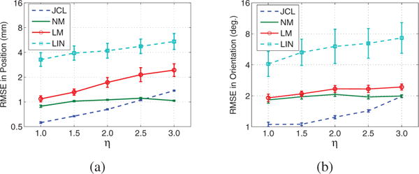
The average tracking accuracies with different speed levels for different methods: (a) RMSE in position vs. speed; (b) RMSE in position vs. speed. The error bars represent standard errors of the means.

H. Pilot Human Subject Trial

This study was conducted in accordance with the Dept. of Health and Human Services regulations for protection of human subjects. The protocol for this research was approved by the Institutional Review Board of the Georgia Institute of Technology. A healthy male subject, 35 years old, participated in this study. A magnet (diameter: 6.05 mm, thickness: 1.25 mm, weight: 0.09 g, residual induction: 14800 G) was temporarily attached to the upper surface of the subject’s tongue, about 1 cm from the tongue apex, using tissue adhesives. The subject was asked to hold his head stationary against the support as portrayed in Fig. 8a that was captured during the experiment, such that the tracer movements could only be attributed to the tongue motion as opposed to the head motion artifacts. The subject was asked to speak single words “lips [lips]” and “sights [saits]”, which consist of vowels and consonants and take 1.13 s and 1.20 s, respectively. When we performed JCL, we also used the magnetic field data that were recorded before and after the speaking of each word to avoid overfitting. The total data length we used for each word is 300, i.e., 3 s. Figs. 8b and 8c show the results of tongue movement trajectories reconstructed by the JCL algorithm for these two words. It can be seen that in /li/, the tongue tip is placed against the middle of the alveolar ridge; for /s/, the tongue tip touches behind the upper teeth; for /p/, the tongue tip slightly drops down with natural open of the mouth; for /ai/, the tongue begins back and low in the mouth, and then moves to a mid-high front; in /ts/, the sibilant affricate, tongue lifts up to stop the air flow entirely, then moves in the direction of the sharp edge of the teeth. The red vectors denote estimated y and z-components of the normalized magnetic moments, i.e., [sinϕsinφ, cosθ], see (1). While speaking the words, the red vectors varied, but generally pointed upwards, since we placed the tracer on the tongue upper surface with north pole faced up.

Fig. 8.

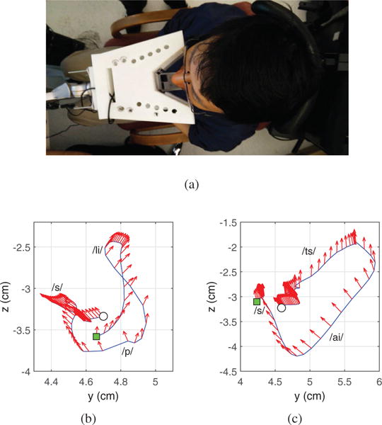
(a) experimental setup for the pilot human subject trial, as well as tracking examples of (b) word “lips” and (c) word “sights” in sagittal plane, the blue lines represent the reconstructed trajectories, the red vectors indicate estimated orientations of the magnetic tracer, the green squares and white circles denote the beginning and end points of tongue trajectories, respectively.

V. Conclusion

In this paper, a joint magnetic calibration and localization algorithm has been proposed to address the bias estimation problem in a tongue tracking system (TTS). The probabilistic relationship between the dynamics of dipole motion and the noise measurements was explicitly modelled. Based on EM criterion, the estimations of magnetic dipole location states and the measurement parameters were alternatively adjusted. By employing curvilinear search, we overcame the problem of orthogonal constraints in updating the sensor rotation matrix. Comprehensive experimental results on 15 datasets demonstrated variations of the calibrated sensor parameters, and showed the proposed method has lower calibration error and higher localization accuracy than the existing approaches. In the pilot human subject trial, the tracer trajectories reconstructed by the proposed method reflected the tongue kinematics during speech. We intend to study sensor selection algorithms to optimize the configuration of TTS and accelerate the computation of the proposed method. We will also conduct additional experiments on both healthy subjects and those with speech impairments.

Biographies

Jun Lu received the Ph.D. degree in electronic engineering from South China University of Technology, Guangzhou, China, in 2008. In 2009 and 2010, he was a post doctor at Center for Brain Computer Interfaces and Brain Information Processing, South China University of Technology, Guangzhou, China, where he has worked on signal processing and machine learning. Since 2011, he has been a Researcher in the School of Automation, Guangdong University of Technology, Guangzhou, China.

Zhongtao Yang received B.S and Master degrees in Electrical and Computer Engineering from Georgia Institute of Technology in 2015, and 2016 respectively. He was a research assistant at GT-Bionics Lab for two years. Currently he is an employee at Amazon, Inc. Seattle, WA, 98121.

Klaus Okkelberg received the B.S. degree in electrical engineering from the Pennsylvania State University in 2011 and the M.S. degree in electrical engineering from the University of New Orleans in 2014. He is currently in the GT-Bionics Lab and working towards the Ph.D. degree in electrical and computer engineering at the Georgia Institute of Technology.

Maysam Ghovanloo (S’00–M’04–SM’10) received the B.S. degree in electrical engineering from the University of Tehran, and the M.S. degree in biomedical engineering from the Amirkabir University of Technology, Tehran, Iran in 1997. He also received the M.S. and Ph.D. degrees in electrical engineering from the University of Michigan, Ann Arbor, in 2003 and 2004. Dr. Ghovanloo developed the first modular Patient Care Monitoring System in Iran where he also founded a startup to manufacture physiology and pharmacology research laboratory instruments. From 2004 to 2007 he was an Assistant Professor in the Department of ECE at the North Carolina State University, Raleigh, NC. Since 2007 he has been with the Georgia Institute of Technology, School of Electrical and Computer Engineering, where he is a Professor and the founding director of the GT-Bionics Lab. He has 8 issued patents and authored or coauthored more than 200 peer-reviewed conference and journal publications on implantable microelectronic devices, integrated circuits and micro-systems for IMD applications, and modern assistive technologies.

References

- 1.Katz WF, McNeil MR. Studies of articulatory feedback treatment for apraxia of speech based on electromagnetic articulography. SIG 2: Perspectives on Neurophysiology and Neurogenic Speech and Language Disorders. 2010 Oct.20(3):73–79. [Google Scholar]
- 2.Yano J, et al. Effect of visual biofeedback of posterior tongue movement on articulation rehabilitation in dysarthria patients. Journal of Oral Rehabilitation. 2015 Mar;42(8):571–579. doi: 10.1111/joor.12293. [DOI] [PubMed] [Google Scholar]
- 3.Ouni S. Tongue control and its implication in pronunciation training. Computer Assisted Language Learning. 2014 May;27(5):439–453. [Google Scholar]
- 4.Katz WF, Mehta S. Visual feedback of tongue movement for novel speech sound learning. Frontiers in Human Neuroscience. 2015 Nov;9 doi: 10.3389/fnhum.2015.00612. [DOI] [PMC free article] [PubMed] [Google Scholar]
- 5.Yang M, et al. Extraction of tongue contour in x-ray videos. IEEE International Conference on Acoustics, Speech and Signal Processing (ICASSP) IEEE. 2013:1094–1098. [Google Scholar]
- 6.Remijn L, et al. Ultrasound imaging for analyzing lateral tongue movements during mastication in adults with cerebral palsy compared with adults without oral motor disabilities. Ultrasound in Medicine & Biology. 2015 Mar;41(6):1784–1793. doi: 10.1016/j.ultrasmedbio.2015.02.007. [DOI] [PubMed] [Google Scholar]
- 7.Badin P, et al. Development and implementation of fiducial markers for vocal tract mri imaging and speech articulatory modelling. Interspeech. 2013:1321–1325. [Google Scholar]
- 8.Ji A, et al. The electromagnetic articulography mandarin accented english (EMA-MAE) corpus of acoustic and 3d articulatory kinematic data. IEEE International Conference on Acoustics, Speech and Signal Processing (ICASSP) IEEE. 2014:7719–7723. [Google Scholar]
- 9.Farajidavar A, et al. A comprehensive method for magnetic sensor calibration: A precise system for 3-D tracking of the tongue movements. Annual International Conference of the IEEE Engineering in Medicine and Biology Society (EMBS) IEEE. 2012:1153–1156. doi: 10.1109/EMBC.2012.6346140. [DOI] [PMC free article] [PubMed] [Google Scholar]
- 10.Cheng C, et al. Towards a magnetic localization system for 3-D tracking of tongue movements in speech-language therapy. Annual International Conference of the IEEE Engineering in Medicine and Biology Society(EMBS) IEEE. 2009:563–566. doi: 10.1109/IEMBS.2009.5334058. [DOI] [PMC free article] [PubMed] [Google Scholar]
- 11.Huo X, et al. A magneto-inductive sensor based wireless tongue-computer interface. IEEE Transactions on Neural Systems and Rehabilitation Engineering. 2008 Nov;16(5):497–504. doi: 10.1109/TNSRE.2008.2003375. [DOI] [PMC free article] [PubMed] [Google Scholar]
- 12.Huray PG. Maxwell’s Equations. Hoboken: Wiley-IEEE Press; 2009. Static magnetic fields; pp. 266–290. ch. 6. [Google Scholar]
- 13.Hu C, et al. A linear algorithm for tracing magnet position and orientation by using three-axis magnetic sensors. IEEE Transactions on Magnetics. 2007 Dec;43(12):4096–4101. [Google Scholar]
- 14.Nara T, et al. A closed-form formula for magnetic dipole localization by measurement of its magnetic field and spatial gradients. IEEE Transactions on Magnetics. 2006 Sep;42(10):3291–3293. [Google Scholar]
- 15.Nara T, et al. Properties of the linear equations derived from euler’s equation and its application to magnetic dipole localization. IEEE Transactions on Magnetics. 2012 Oct;48(11):4444–4447. [Google Scholar]
- 16.Wang X, et al. A localization method using 3-axis magnetoresistive sensors for tracking of capsule endoscope. Annual International Conference of the IEEE Engineering in Medicine and Biology Society (EMBS) IEEE. 2006:2522–2525. doi: 10.1109/IEMBS.2006.260711. [DOI] [PubMed] [Google Scholar]
- 17.Yang W, et al. A six-dimensional magnetic localization algorithm for a rectangular magnet objective based on a particle swarm optimizer. IEEE Transactions on Magnetics. 2009 Jul;45(8):3092–3099. [Google Scholar]
- 18.Hu C, et al. A cubic 3-axis magnetic sensor array for wirelessly tracking magnet position and orientation. IEEE Sensors Journal. 2010 Apr;10(5):903–913. [Google Scholar]
- 19.Song S, et al. 6-d magnetic localization and orientation method for an annular magnet based on a closed-form analytical model. IEEE Transactions on Magnetics. 2014 Sep;50(9):1–11. [Google Scholar]
- 20.Shen H-M, et al. Real-time orientation-invariant magnetic localization and sensor calibration based on closed-form models. IEEE Magnetics Letters. 2015 Aug;6:1–4. [Google Scholar]
- 21.Li Y, et al. Numeric calculation for near field of permanent magnet. Information and Automation (ICIA), 2013 IEEE International Conference on IEEE. 2013:499–504. [Google Scholar]
- 22.Beravs T, et al. Magnetometer calibration using Kalman filter covariance matrix for online estimation of magnetic field orientation. IEEE Transactions on Instrumentation and Measurement. 2014;63(8):2013–2020. [Google Scholar]
- 23.Springmann JC, Cutler JW. Attitude-independent magnetometer calibration with time-varying bias. Journal of Guidance, Control, and Dynamics. 2012;35(4):1080–1088. [Google Scholar]
- 24.Tasko SM, Westbury JR. Speed–curvature relations for speech-related articulatory movement. Journal of Phonetics. 2004 Jan;32(1):65–80. [Google Scholar]
- 25.Löfqvist A. Tongue movement kinematics in long and short japanese consonants. The Journal of the Acoustical Society of America. 2007 Jul;122(1):512–518. doi: 10.1121/1.2735102. [DOI] [PMC free article] [PubMed] [Google Scholar]
- 26.Yunusova Y, et al. Tongue movements and their acoustic consequences in amyotrophic lateral sclerosis. Folia Phoniatrica et Logopaedica. 2012 Apr;64(2):94–102. doi: 10.1159/000336890. [DOI] [PMC free article] [PubMed] [Google Scholar]
- 27.Dempster AP, et al. Maximum likelihood from incomplete data via the EM algorithm. Journal of the Royal Statistical Society Series B (Methodological) 1977 Jan;:1–38. [Google Scholar]
- 28.Sarkka S. Unscented rauch–tung–striebel smoother. IEEE Transactions on Automatic Control. 2008 Apr;53(3):845–849. [Google Scholar]
- 29.Wen Z, Yin W. A feasible method for optimization with orthogonality constraints. Mathematical Programming. 2013 Dec;142(1–2):397–434. [Google Scholar]
- 30.Lima EA, et al. The magnetic inverse problem. The SQUID Handbook: Applications of SQUIDs and SQUID Systems. 2006;II:139–267. [Google Scholar]
- 31.Olivier LE, et al. Dual particle filters for state and parameter estimation with application to a run-of-mine ore mill. Journal of Process Control. 2012 Mar;22(4):710–717. [Google Scholar]
- 32.Zhao Z, et al. Parameter estimation in batch process using em algorithm with particle filter. Computers & Chemical Engineering. 2013 Oct;57:159–172. [Google Scholar]
- 33.Särkkä S. Bayesian filtering and smoothing. Vol. 3 Cambridge University Press; 2013. [Google Scholar]
- 34.Kokkala J, et al. Sigma-point filtering based parameter estimation in nonlinear dynamic systems. arXiv preprint arXiv:1504.06173. 2015 Apr; [Google Scholar]
- 35.Sage AP, Melsa JL. Estimation theory with applications to communications and control. DTIC Document, Tech Rep. 1971 Oct; [Google Scholar]
- 36.Julier SJ, Uhlmann JK. Unscented filtering and nonlinear estimation. Proceedings of the IEEE. 2004 Mar;92(3):401–422. [Google Scholar]
- 37.Lin C-Y, Tomizuka M. International Conference of the ASME Dynamic Systems and Control. American Society of Mechanical Engineers; 2015. Estimating rigid transformation with correlated observations. [DOI] [Google Scholar]
- 38.Edelman A, et al. The geometry of algorithms with orthogonality constraints. SIAM journal on Matrix Analysis and Applications. 1998 Jun;20(2):303–353. [Google Scholar]
- 39.Cayley A. Sur quelques propriétés des déterminants gauches. Journal für die reine und angewandte Mathematik. 1846;32:119–123. [Google Scholar]
- 40.Barzilai J, Borwein JM. Two-point step size gradient methods. IMA Journal of Numerical Analysis. 1988 Aug;8(1):141–148. [Google Scholar]
- 41.Zhang H, Hager WW. A nonmonotone line search technique and its application to unconstrained optimization. SIAM Journal on Optimization. 2004 May;14(4):1043–1056. [Google Scholar]
- 42.Slabaugh GG. Computing euler angles from a rotation matrix. Retrieved on August. 1999 Aug;6(2000):39–63. [Google Scholar]