Covariate Selection for Association Screening in Multi-Phenotype Genetic studies

Abstract

Testing for associations in big data faces the problem of multiple comparisons, with true signals difficult to detect on the background of all associations queried. This is particularly true in human genetic association studies where phenotypic variation is often driven by numerous variants of small effect. The current strategy to improve power to identify these weak associations consists of applying standard marginal statistical approaches and increasing study sample sizes. While successful, this approach does not leverage the environmental and genetic factors shared between the multiple phenotypes collected in contemporary cohorts. Here we develop Covariates for Multi-phenotype Studies, an approach that improves power when correlated variables have been measured on the same samples. Our analyses over real and simulated data provide direct support that correlated phenotypes can be leveraged to achieve dramatic increases in power, often surpassing the power equivalent of a two-fold increase in sample size.

Introduction

Performing agnostic searches for association between pairs of variables in large-scale data, using either common statistical techniques or machine learning algorithms, faces the problem of multiple comparisons. This is particularly true for genetic association studies, where contemporary cohorts have access to millions of genetic variants as well as a broad range of clinical factors and biomarkers for each individual. With billions of candidate associations, the identification of a true association of small magnitude is extremely challenging. Standard analysis approaches currently consists of looking at the data in one dimension (i.e. testing a single outcome with each of the millions of candidate genetic predictors) and applying univariate statistical tests – the commonly named GWAS (genome-wide association study) approach^{1, 2}. To increase power, GWAS rely on increasing sample size in order to reach the multiple comparisons adjusted significance level. The largest studies to date, including hundreds of thousands of individuals across dozens of cohorts, have pushed the limit of detectable effect sizes. For example, researchers are now reporting genetic variants explaining less than 0.01% of the total variation of body mass index (BMI)³.

In addition to the substantial financial costs of collecting and genotyping large cohorts, this brute force approach has practical limits. More importantly, this approach does not leverage the large amount of additional phenotypic and genomic information measured in many studies. Joint analyses of multiple phenotypes with each predictor of interest (e.g. Manova, MultiPhen)^4–6 offer a gain in power, but have three major drawbacks. First, a significant result can only be interpreted as an association with any one of the phenotypes. While this is useful information for screening purposes, it is insufficient to identify specific genotype-phenotype associations⁶. Second, it makes the replication process difficult, since all genotype-phenotype pairs must be considered. Third, joint tests have lower power than univariate tests when only a small proportion of the phenotypes are associated with the tested genetic variant. This is a simple problem of dilution; a small number of true associations mixed with many null phenotypes will reduce power.

In this work, we develop CMS (covariates for multi-phenotype studies), a method that improves association test power in multi-phenotype studies, while providing the resolution of univariate tests. When testing for association between a genotype and a phenotype CMS allows the other collected correlated phenotypes to serve as covariates. The core of the method is a principled approach to selecting a set of these covariates that are correlated with the phenotype, but not with the genotype, thereby reducing phenotypic variance independent of the genotype and concomitantly increasing power. We show via application to simulated and real data sets that CMS scales to thousands of phenotypes, produces gains in power equivalent to a two- to three-fold increase in sample size, and outperforms other recently proposed multi-phenotype approaches with univariate resolution including a Bayesian approach (mvBIMBAM⁷), and dimensionality reduction approaches (PCA⁸, PEER⁹).

Results

Covariates as proxy for unmeasured causal factors

The objective of this work is to develop a method that keeps the resolution of univariate analysis when testing for association between an outcome Y and candidate predictor X, but takes advantage of other available covariates $C=\left(C_1,C_2,\dots C_m\right)$ to increase power. Consider the inclusion of covariates correlated with the outcome in a standard regression framework. This may increase the signal-to-noise ratio between the outcome and the candidate predictor when testing: $Y=X+C_L$, where $C_L\subset C$. The selection of which covariates $C_i$ are relevant to a specific association test is usually based on causal assumptions^{10, 11}. Epidemiologists and statisticians commonly recommend the inclusion of two types of covariates when testing for association between X and Y: those that are potential causal factors of the outcome and independent of X, and those that may confound the association signal between X and Y, i.e. variables such as principal components (PCs) of genotypes or covariates that capture undesired structure in the data that can lead to false associations¹². All other variables that vary with the outcome because of shared risk factors are usually ignored. However, those variables carry information about the outcome, and more precisely about the risk factors of the outcome. Because they potentially share dependencies with the outcome, they can be used as proxies for unmeasured risk factors. As such, they can be incorporated in $C_L$ to improve the detection of associations between X and Y. However, when these variables depend on the predictor X, using them as covariates can lead to both false positive and false negative results depending on the underlying causal structure of the data.

The presence of interdependent explanatory variables, also known as multicollinearity¹³, can induce bias in the estimation of the predictor’s effect on the outcome. We recently discussed this issue in the context of genome-wide association studies that adjusted for heritable covariates¹⁴. To illustrate this collider bias, consider first the simple case of two independent covariates $U_1$ and $U_2$ that are true risk factors of Y. When testing for association between X and Y, adjusting for $U_1$ and $U_2$ can increase power, because the residual variance of Y after the adjustment is smaller while the effect of X is unchanged (Fig. 1a), i.e. the ratio of the outcome variance explained by X over the residual variance is larger after removing the effect of $U_1$ and $U_2$. However, in practice, true risk factors of the outcome are rarely known. Consider instead the more realistic scenario where $U_1$ and $U_2$ are unknown but a covariate C, which also depends on those risk factors, has been measured. Because of their shared etiology, Y and C display positive correlation, and when X is not associated with C, adjusting Y for C increases power to detect ( $Y,X$) associations (Fig. 1b). Problems arise when C is associated with X. In this case adjusting Y for C biases the estimation of the effect of X on Y, decreasing power when the effect of X is concordant between C and Y (Fig. 1c), and inducing false signal when the effect is discordant (in opposite direction or when X is not associated with Y, Fig. 1d). The same principles apply when including multiple covariates correlated with the outcome.

Figure 1. Variance components of adjusted variables.

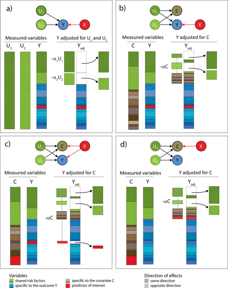
We illustrate the components of the variance of an outcome Y before and after adjusting for other variables. The predictor of interest, X, is displayed in red. In (a), the adjusting variables (U₁ and U₂) are true causal factors that have direct effects on Y, therefore adjusting Y for U₁ and U₂ reduces the variance of Y. In (b) the true factors are not measured but a variable C influenced by U₁ and U₂, is measured. Adjusting Y for C reduces the residual variance of Y, but also introduces a component of the variance specific to C. In (c) the covariate shares factors with Y, but is also influenced by X. When the effect of X on C is concordant with the effect of X on Y, this can induce a power loss. In (d) Y is not associated with the predictor and adjusting for C can induce false association signal by introducing the effect of X into the residual of Y.

When none of the covariates depend on the predictor (Fig. 1a-b), their inclusion in a regression can reduce the variance of the outcome without confounding, leading to increased statistical power while maintaining the correct null distribution. This gain in power can be easily translated in terms of a sample size increase. The noncentrality parameter (ncp) of the standard univariate chi-square test between X and Y is $nc{p}_{XY}=N\times {\pi }_X^2/\left({\sigma }_Y^2-{\pi }_X^2\right)$ where N, ${\sigma }_Y^2$ and ${\pi }_X^2$are the sample size, the total variance of the outcome Y, and the squared correlation between X and Yrespectively. When reducing ${\sigma }_Y^2$ by a factor $\gamma$ through covariate adjustment, and assuming the effect of X on Y is small, so that ${\sigma }_Y^2-{\pi }_X^2\approx {\sigma }_Y^2$, $nc{p}_{XY}$ can be approximated by $N\times {\pi }_X^2/\left({\sigma }_Y^2/\gamma \right)=\left(N/\gamma \right)\times \left({\pi }_X^2/{\sigma }_Y^2\right)$. For example, when the covariates explain 30% of the variance of Y, the power of the adjusted test is equivalent to analyzing approximately a 1.4 fold larger sample size (as compared to the unadjusted test). When covariates explain 80% of the phenotypic variance –a realistic proportion in some genetic datasets examined below– the power gain is equivalent to a five-fold increase in sample size (Fig. 2a).

Figure 2. Examples of shared variance in real data and equivalent increases in sample size.

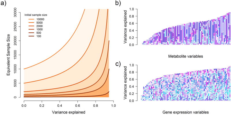
Panel (a) shows the equivalent increase in sample size as a function of the variance of the outcome explained by covariates assuming initial sample sizes ranging from 100 to 10,000. Panels (b) and (c) show the distribution of variance explained by other variables for 79 metabolites from the PANSCAN study, and a random sub-sample of expression abundance estimates from 79 genes in the gEUVADIS study. The size of the bar corresponds to the total variance explained of each outcome by other available covariates, while the relative contribution of these covariates to each outcome is illustrated with different sets of random colors for each bar.

Selecting covariates for each outcome-predictor pair

The central problem that must be solved is how to select a subset of the available covariates to optimize power while preventing induction of false positive associations between the outcome and the predictor. To do this, all covariates associated with the outcome should be included except those also associated with the predictor. A naïve solution would consist of filtering out covariates based on a p-value threshold from the association test between each covariate and the predictor (e.g. removing predictors with a predictor-covariate association p-value < 0.05). However, unless the sample size is infinitely large, type I covariates (i.e. covariates associated with the predictor) will be included. Furthermore, such a filtering also implies that some type II covariates (i.e. covariates not associated with the predictor) will be removed because they incidentally pass the p-value threshold. Interestingly, removing type II covariates using this approach not only results in a sub-optimal test, it also induces an inflated false positive rate (Supplementary Fig. 1). In brief, when the outcome and the covariate are correlated, low predictor-covariate p-value implies low predictor-outcome p-value. As a result, the p-value distribution from the subset of predictor-outcome unadjusted statistics (i.e. those for which the predictor-covariate p-value is below the threshold) is enriched for low p-value, resulting in an overall type I error inflation for the approach (Supplementary Note and Supplementary Fig. 2).

In this work, we develop a computationally efficient heuristic to improve the selection of type II covariates while removing type I covariates that we refer further to as CMS (Covariates for Multi-Phenotype Studies). We present an overview of the approach, with complete details of the algorithm provided in the online Methods and the Supplementary Note.

Let $\widehat{\delta }$ and $\widehat{\beta }$ be the marginal estimated regression coefficients between $X$ and C, and between X and $Y$ (not adjusted for C) respectively, and let $\widehat{\gamma }$ be the estimated correlation between Y and C. Naive p-value based filtering, i.e. unconditional filtering on $\widehat{\delta }$, assumes that under the null ( $\delta =0$) $\widehat{\delta }$ is normally distributed with $\mathbb{E}\left(\widehat{\delta }\right)=0$ and variance $1/n$, where n is the sample size. The central advance of CMS is to additionally use the expected mean and variance of $\widehat{\delta }$ conditional on $\widehat{\beta }$ under a complete null model ( $\delta =\beta =0$). We show that this can be approximated as: $\mathbb{E}\left(\widehat{\delta }|\widehat{\beta }\right)\approx \widehat{\beta }\widehat{\gamma }$ and $\mathrm{var}\left(\widehat{\delta }|\widehat{\beta }\right)\approx \mathrm{var}\left(\widehat{\delta }-\widehat{\beta }\widehat{\gamma }\right)=\left(1-{\widehat{\gamma }}^2\right)/n$ (Supplementary Note, and Supplementary Fig. 3).

The bias observed from naïve univariate p-value filtering (Supplementary Fig. 1) is induced by the misspecification of the expected mean and variance of the predictor-covariate effect estimate when the predictor is associated with neither the outcome, nor the covariates. Figure 3a illustrates $\widehat{\delta }$ inclusion area for a p-value threshold of 5% –i.e. if $\widehat{\delta }$ is outside the inclusion area, the covariate $C$ is filtered out –based on the unconditional distribution. As shown in Supplementary Table 1 and Supplementary Figure 4, which describes the simple case of a single covariate, using the distribution of $\widehat{\delta }$ conditional on $\widehat{\beta }$ to select covariates is also poor solution, resulting in a deflated test statistic for $\widehat{\beta }$ due to an overestimation of the standard error of $\widehat{\beta }$ when adjusting for the selected covariates. The improvement from CMS is derived from defining the inclusion area as a combination of the unconditional and conditional distributions of $\widehat{\delta }$ (Figure 3b,c). This solves the inflation observed in Supplementary Fig. 1 and leads to a valid test under the complete null model with a variable number of available covariates (see Supplementary Fig. 3 and Supplementary Table 1).

Figure 3. Conditional and unconditional distribution.

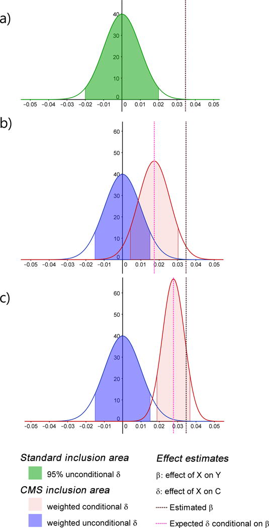
Example of inclusion area based on the distribution of $\widehat{\delta }$, the estimated effect between the predictor X and the covariate C under the null hypothesis of no association between X and C ( $\delta =0$) and no association between X and the outcome Y ( $\beta =0$). (a) presents the standard 95% confidence interval (green area) corresponding to p-value <0.05 unconditional on $\widehat{\beta }$. (b) and (c) show both the unconditional (blue curve) and conditional (pink curve) distribution of $\widehat{\delta }$. CMS combines the two, setting an inclusion area (blue+pink shaded), while weighting both interval by a factor depending on the correlation between Y and C, which equals 0.5 in (b) and 0.8 in (c). Plots were drawn assuming all variables are standardized, using a sample size of 10,000, an overall variance of Y explained of 0.7, $\widehat{\beta }=0.035$ and a multivariate test of association between all covariates and Y with a p-value ( $p_{\mathrm{MUL}}$) of 0.3.

Finally, to reduce the risk of false positives, the algorithm scales inclusion areas on the basis of total amount of the outcome’s variance explained by $C_{l\in L}$ and $\widehat{\beta }$. To further improve the performance of filtering covariates we also consider omnibus association test between $C_{l\in L}$ and Y, which is more effective when multiple covariates have small to moderate effects (see Supplementary Note).

Simulated data analysis and method comparisons

We first assessed the performance of the proposed method through a simulation study in which we generated series of multi-phenotype datasets over an extensive range of parameter settings (see online Methods and Supplementary Note). Each dataset included n individuals genotyped at a single nucleotide polymorphism (SNP) with minor allele frequency (MAF) drawn uniformly from [0.05, 0.5], a normally distributed phenotype Y, and $m=\left[10, 40, 80\right]$ correlated covariates $C=\left(C_1,C_2,\dots C_m\right)$. Under the null, the SNP does not contribute to the phenotype and under the alternate the SNP contributes to the phenotype under an additive model. In some datasets, the SNP also contributes to a fraction $\pi =\left[0\text{\%},15\text{\%},35\text{\%}\right]$ of the covariates. These are the covariates, which we wish to identify and filter out of the regression. We considered sample sizes n of 300, 2,000 and 6,000, we varied $r_C^2$, the variance of Y explained by C, from 25% to 75%. We varied the effect of the predictor on Y and C, when relevant, from almost undetectable (i.e. median ${\chi }^2=3$) to relatively large (i.e. median ${\chi }^2=20$). For each choice of parameters, we generated 10,000 replicates and performed four association tests: (unadjusted) linear regression (LR), linear regression with covariates included based on p-value filtering at an $\alpha$ threshold of 0.1 (FT), CMS, and an oracle method that includes only the covariates not associated with the SNP (OPT), this being the optimal test regarding our goal. We considered a total of 432 scenarios and as shown in Figure 4 and Supplementary Tables 2-4 the type I error rate of CMS is well calibrated across parameter ranges. Note that we did not consider strategies which include all $C_{l=1\dots m}$ variables as covariates, MANOVA, or “reverse regression” (i.e. MultiPhen)⁵, as these approaches lead to substantial inflation of type I error rate (see Supplementary Fig. 5).

Figure 4. Power and robustness.

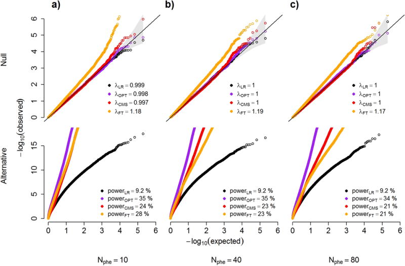
QQ plots under the null and alternate distributions of p-values from a series of simulations. We compare four statistical tests: a standard marginal univariate test (LR); the optimally adjusted test (OPT) that includes as covariates only the outcomes not associated with the predictor; CMS; and a univariate test that include as covariate all outcomes with a p-value for association with the predictor above 0.1 (FT). Grey boxes show the genomic inflation factor ${\lambda }_{GC}$ for the null models (upper panels), and estimated power at an α threshold of 5×10⁻⁷ (to correct for 100,000 tests) for the alternative model (lower panels). Null models also include the 95% confidence interval of the −log₁₀(p-values), displayed as a grey cone around the diagonal. Simulations were taken from 100,000 datasets including 10 (a), 40 (b) and 80 (c) outcomes under a null model (upper panels), where a predictor of interest is not associated with a primary outcome but is associated with either 0%, 15% or 35% of the other outcomes with probability 0.75, 0.2 and 0.05 respectively, and under the alternative (lower panels), where the predictor is associated with the primary outcome only. The variance of the primary outcome that can be explained by the other outcomes was randomly chosen from [25%, 50%, 75%] with equal probability.

We compared the performances of CMS against other recently proposed multi-phenotype approaches including mvBIMBAM. The CMS approach was more than 100 fold faster than mvBIMBAM and the two methods showed similar accuracy when compared using ROC curves (Supplementary Fig. 6). We also considered data reduction techniques aimed at modelling hidden structure. For each dataset we tested the association between the primary outcome and the genotype while adding principal components (PCs) or PEER factors. We observed increasing type I error rates when increasing the number of PCs or PEER factors in the model (Supplementary Figure 7). Furthermore, at a fixed false positive rate, when we applied CMS on top PEER factors, we found that CMS substantially increases power above those gains available from PEER (Supplementary Fig. 8 and Supplementary Note).

Real data analysis

We first analyzed a set of 79 metabolites measured in 1192 individuals genotyped at 668 candidate SNPs. We derived the correlation structure between these metabolites (Fig. 2b and Supplementary Fig. 9)³ and estimated the maximum gain in power that can be achieved by our approach in these data. The proportion of variance of each metabolite explained by the other metabolites varied between 1% and 91% (Fig. 2b). This proportion is higher than 50% for two thirds of the metabolites, equivalent to a two-fold increase in sample size. For 10% of the metabolites, other variables explain over 80% of the variance, corresponding to a five-fold increase in sample size. In such cases, predictors explaining less than 1% of metabolite’s variation can change from undetectable (power<1%) to fully detectable (power>80%).

We performed a systematic screening for association between each SNP and each metabolite, using both a standard univariate linear regression adjusting for potential confounding factors and using CMS to identify additional covariates. Overall, both tests showed correct ${\lambda }_{GC}$ (Supplementary Fig. 10a). We focused on associations significant after Bonferroni correction (P < 9.5×10⁻⁷ corresponding to the 52,772 tests performed). The standard unadjusted approach (LR) detected 5 significant associations. In comparison, the CMS approach identifies 10 associated SNPs (Table 1), including four of the five associations identified by LR. In most cases the p-value of CMS was dramatically lower (e.g. 1000 fold smaller for rs780094 – alanine). Comparing these results to four independent GWAS metabolite scans of larger sample size (N equal 8,330, 7,824, 2,820, and 2,076 for Finnish¹⁵, KORA+TwinsUK,^{16, 17} and FHS,¹⁸ respectively), we found that all metabolite/gene associations only identified by CMS replicated (Supplementary Table 5).

Table 1.

Identified signals from the association test between 79 metabolites and 668 candidate SNPs.

Chr	SNP	Gene	Outcome	P-value			Known from study
				PLR	PCMS	SSincr
1	rs477992	PHGDH	serine	6.2×10−5	1.4×10−7	2.15	KORA+TwinsUK16/FHS18
2	rs2216405	near CPS1, LANCL1	glycine	4.1×10−26	2.3×10−33	1.56	KORA+TwinsUK16/FHS18
			serine	3.7×10−5	6.4×10−10	1.76	KORA+TwinsUK16/FHS18
			creatine	7.6×10−8	4.8×10−9	1.34	KORA+TwinsUK16/FHS18
			acetylglycine	2.2×10−8	3.1×10−9	1.44	KORA+TwinsUK16
2	rs780094	GCKR	alanine	6.1×10−5	4.0×10−8	2.06	KORA+TwinsUK16/FHS18/Finnish15
4	rs1352844	GC	lactose	6.1×10−7	6.3×10−6	2.06
10	rs7094971	SLC16A9	carnitine	2.9×10−10	1.1×10−15	2.01	KORA+TwinsUK16/FHS18
			acetylcarnitine	1.4×10−6	9.4×10−13	2.36	KORA+TwinsUK16
12	rs2657879	GLS2	glutamine	3.1×10−5	4.2×10−10	2.50	KORA+TwinsUK16/Finnish15
16	rs6499165	SLC7A6	lysine	2.6×10−5	7.5×10−10	3.00	KORA+TwinsUK16

There was 79 metabolites tested for association with 668 SNPs, so a total of 52104 tests. P-value threshold accounting for multiple testing is 9.5×10-7. Significant p-values are indicated in bold.

Abbreviation: P_LR is the p-value for the standard unadjusted univariate test of each single phenotype with each single SNP; P_CMS is the p-value from the CMS algorithm; SS_incr is the equivalent sample size increase achieved after adjusting for covariates selected by the CMS algorithm.

Sample size of the replication was 8,330, 7,824, and 2,076 for Finnish¹⁵, KORA+TwinsUK^{16, 17}, and FHS¹⁸ studies, respectively

This analysis confirms the power of CMS, highlighting its ability to identify variants with much smaller sample size. Interestingly, the only association identified by the unadjusted analysis (lactose and GC, P=6.1×10⁻⁷) and not confirmed by CMS (P=6.3×10⁻⁶) was also the only one that did not replicate in the larger studies. Note that in the analysis presented in Table 1, we followed the identical analysis approach of the previous studies and did not adjust for either PCs or PEER factors⁹. However, adjusting did not qualitatively change the results. For example, we considered adjusting for 5, 10, and 20 PCs and obtained 11, 15 and 17 hits for CMS and 9, 11, and 5 hits for LR with PC covariates (Supplementary Table 6). The overall replication rate was lower when including PCs, consistent with the higher false positive rate we observed in our simulations.

We then considered genome-wide cis-eQTL mapping in RNA-seq data from the gEUVADIS study. Gene expression is a particularly compelling benchmark, as the gold standard analyses already use an adjustment strategy to account for hidden factors in eQTL GWAS^{9, 19}. Here we used the PEER approach⁹ to derive hidden factors, as this method was applied in the original analysis²⁰. After stringent quality control the data included 375 individuals of European ancestry with expression estimated on 13,484 genes, of which 11,675 had at least one SNP with a MAF ≥ 5% within 50kb of the start and end sites.

We observed that expressions levels between genes were highly correlated (Fig. 2c), an ideal scenario for CMS. We first performed a standard cis-eQTL screening using linear regression (LR), testing each SNP within 100kb of each available gene for association with overall normalized RNA level while adjusting for 10 PEER factors, for a total of ~1.3 million tests. Then, we applied CMS to identify, for each test, which other gene’s RNA levels could be used as covariates on top of the PEER factors. As shown in Supplementary Figure 10b, both LR and CMS showed large number of highly significant associations. For comparison purposes we plotted the most significant SNP per gene obtained with the standard approach against those obtained with CMS in Figure 5. As shown in this figure, 2,725 genes had a least one SNP significant with both methods, and 56 genes were identified by the standard approach only. Conversely 657 genes were found only with CMS, corresponding to a 24% increase in detection of cis-eQTL loci. This indicates that by being gene/SNP specific, CMS is a priori able to recover substantial additional variance, allowing for increased power (Table 2 and Supplementary Table 7).

Figure 5. Analysis of the gEUVADIS data.

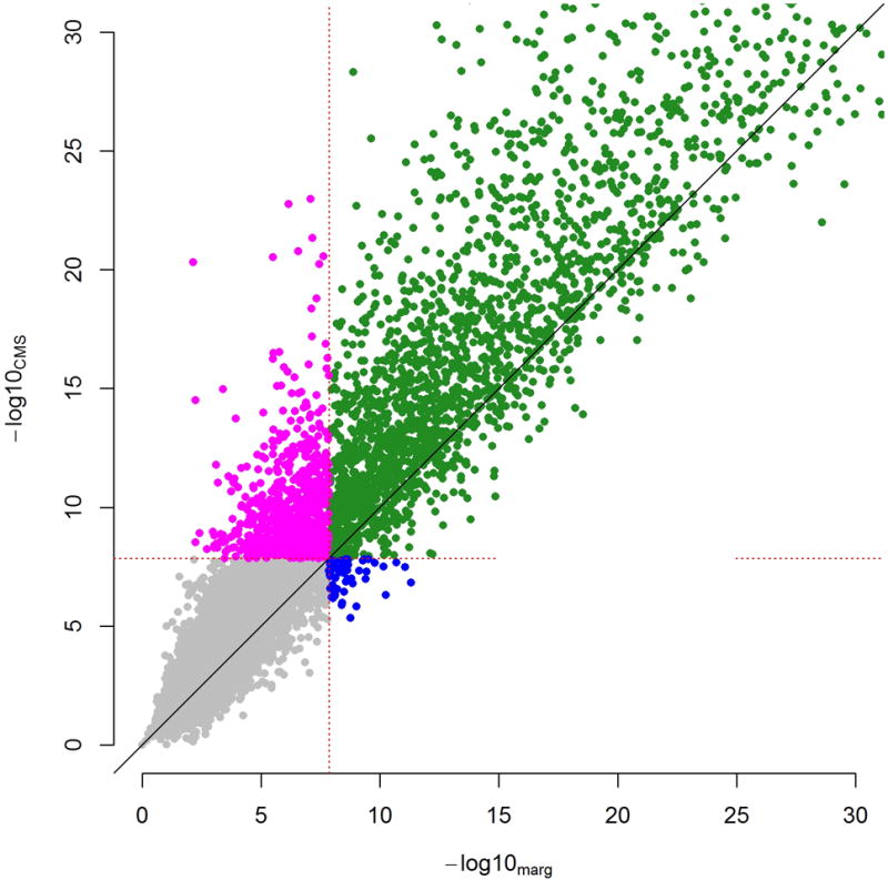
−log₁₀(p-values) of the most significant SNP per gene obtained by CMS (y-axis) and linear regression (LR, x-axis) from a genome-wide cis-eQTL mapping of 11,675 genes in 375 individuals from the gEUVADIS study. For illustration purposes we truncated the plots at −log₁₀(p-value)=30. Both CMS and LR adjusted for 10 PEER factors, while the CMS analysis also included 0 to 50 additional covariates per SNP/gene pair tested. We considered a stringent significance threshold of 1.4×10⁻⁸ to account for the approximately 3.5 million tests and derived the number of gene showing at least one cis-eQTL with LR only (blue), CMS only (red), both approaches (turquoise), or neither (grey).

Table 2.

Replication of association from the cis-eQTL screening in GEUVADIS.

Approach	# Disc.a	SNPb	%Rep.c	Replication per Tissue
				Fibr.	LCL	Tcell	Brain	Bcell	Mon.	Liv.	Adi.	Skin	Blood
LR & CMS	2725	LR	34.7%	1	737	4	27	20	69	33	137	125	185
		CMS	35.9%	3	770	2	26	20	73	28	147	133	175
LR only	56	LR	21.8%	0	5	0	0	1	0	0	3	4	3
		CMS	24.1%	0	8	0	0	1	0	0	2	2	3
CMS only	657	LR	20.2%	1	79	0	1	6	7	3	14	7	35
		CMS	19.6%	1	78	0	1	5	6	2	16	11	35
None	8237	LR	7.0%	1	185	1	2	9	38	10	61	53	245
		CMS	7.2%	1	199	2	4	8	46	7	81	62	258

^aNumber of SNP-gene association with p-value below the Bonferroni corrected significance threshold.

^bSNP used for the replication analysis

^cPercentage of SNP-gene association replicated, after removing the discovery SNPs that could not be mapped.

Abbreviation: Fibr. = Fibrobalst; Mon.= Monocytes ; Liv.=Liver; Adi.=Adipose

Note that the sum of per-tissue does not equal the number of hits times the % of replication as a given association can be replicated in multiple tissue.

To assess the validity of our results we performed an in-silico replication analysis using two databases of known eQTLs^{21, 22}. We found that 35% of the SNP-gene associations found by both LR and CMS replicated. For the subset of association found only by CMS the replication rate was 20%, similar to the results from the LR only replication, which was 22%. The replication rate was 6% for genes without a CMS or LR association. The replications were primarily in LCL (Table 2), and the replication rate for our study is within the same range as the replication rate from previous LCL studies (Supplementary Table 8), confirming that a substantial number of the additional associations identified by CMS correspond to real signal (see Supplementary Note). Additional GC correction of the p-values using inflation factors form a null experiment ( ${\lambda }_{\mathit{LR}}$=1.01, and ${\lambda }_{\mathit{CMS}}$=1.05, Supplementary Fig. 11) did not qualitatively change the results.

Discussion

Growing collections of high-dimensional data across myriad fields, driven in part by the “big data revolution” and the Precision Medicine Initiative, offer the potential to gain new insights and solve open problems. However, when mining for associations between collected variables, identifying signals within the noise remains challenging. While univariate analysis offers precision, it fails to leverage the correlation structure between variables. Conversely, joint analyses of multiple phenotypes have increased power at the cost of decreased precision. We demonstrated in both simulated and real data that the proposed method, CMS, maintains the precision of univariate analysis, but can still exploit global data structures to increase power. Indeed, in the data sets examined in this study we observed up to a 3-fold increase in effective sample size in both the gene expression and metabolites data thanks to the inclusion of relevant covariates (Supplementary Figure 12).

CMS can be applied generally, but is particularly well suited to the analysis of genetic data for several reasons. First, the genetic architectures of many complex phenotypes are consistent with a polygenic model with many genetic variants of small effect size that are difficult to detect using standard approaches²³. Second, many correlated phenotypes share genetic and environmental variance without complete genetic overlap²⁴. Third, the underlying structure of the genomic data is relatively well understood with an extensive literature on the causal pathway from genotypes to phenotypes through direct and indirect effects on RNA, protein and metabolites (Supplementary Fig. 13 and Supplementary Note). Finally, when the predictors of interests are genetic variants, there is less concern regarding potential confounding factors. The only well-established confounder of genetic data is population structure and this can be easily addressed using standard approaches¹². For other types of data, when the underlying structure of the data is unknown the risk for introducing bias is high.

Several other groups have considered the problem of association testing in high-dimensional data while maintain precision. In genetics, multivariate linear mixed models (mvLMMs) have demonstrated both precision and increases in power when correlated phenotypes are tested jointly. However, mvLMMs are only exploiting the genetic similarity of phenotypes and are not computationally efficient enough to handle dozens of phenotypes jointly⁴. CMS leverages both genetic and environmental correlations and can be easily adapted to hundreds or thousands of phenotypes as we demonstrated here. Instead, we compared CMS to other more related approaches, including the Bayesian approach mvBIMBAM, and adjustment for hidden factors inferred from either principal component analysis or PEER. We found that mvBIMBAM and CMS had very similar accuracy as measured by the AUC, while mvBIMBAM was approximately 100 fold slower, and applicable only to a small number of phenotypes (i.e. <10). As for strategies that reconstruct hidden variables, we found that they can induce false positives²⁵, and are suboptimal compared to CMS. Indeed, the gEUVADIS analysis showed a 24% increase in the detection of eQTL when applied on top of PEER factor adjustment.

There are several caveats to our approach. First, the proposed heuristic is conservative by design to avoid false association signals and so all the available power gain is not achieved. Second, while all simulations we performed show strong robustness, it remains a heuristic as are other methods^{9, 19}. Ultimately, we recommend external replication to validate results and effect size, as is standard in genetic studies. Third, CMS is more computationally intensive than methods such as PCA or PEER. Fourth, CMS assumes that the variables are measured and available on all samples. The current implementation includes a naïve missing data imputation and simple case-scenario simulations showed this strategy has minimum impact on the robustness of CMS (supplementary Fig. 14). However more advanced approaches have been developed²⁶. Fifth, while the principles we leveraged are likely applicable to categorical and binary outcomes (see²⁷ for logistic regression), our algorithm is currently only applicable to continuous outcomes. Sixth, for monogenic disorders, or phenotypes without intermediately measured endophenotypes, CMS is unlikely to result in power gains.

We focused on association screening and aimed at optimizing power and robustness. However, the selection of covariates performed by CMS might carry information about which covariates are operating through specific SNPs. Future work will explore whether output from CMS can generate hypotheses on the underlying causal model. There are other additional improvements not specific to CMS worth exploring. In particular, when multiple phenotypes are considered as outcomes then a multiple test correction penalty must be selected to account for all tests across all phenotypes. In this study, we applied a Bonferroni correction, not accounting for the correlation between outcomes. This is a conservative correction and more powerful approaches are possible²⁸.

Large-scale genomic data have the potential to answer important biological questions and improve public health. However, those data come with methodological challenges. Many questions, such as improving risk prediction or inferring causal relationships rely on our ability to identify associations between variables. In this study, we provide a comprehensive overview of how leveraging shared variance between variables can be used to fulfill this goal. Building on this principle we developed the CMS algorithm, an innovative approach which can dramatically increase statistical power to detect weak associations.

Online Methods

The CMS algorithm

We develop an algorithm to select relevant covariates when testing for association between a predictor X and an outcome Y. For a set of candidate covariates $C=\left(C_1,C_2,\dots C_m\right)$, the filtering is applied on ${\widehat{\delta }}_l$ and $p_l$, the estimated marginal effect of the predictor X on $C_l$ and its associated p-value, respectively. It uses four major features: i) $r_C^2$ the total amount of variance of Y explained by the C ; ii) ${\widehat{(\gamma }}_{\mathit{lu}}^2,{\widehat{\gamma }}_{\mathit{lm}}^2$)the estimated effect of each $C_{l\in 1\dots m}$ on Y and their joint effect respectively; iii) $\widehat{\beta }$, the estimated effect of X on Y from the marginal model $Y~\alpha +\beta X$; and iv) $p_{\text{MUL}}$, the p-value for the multivariate test of all $C_{l=1\dots m}$ and X, which is estimated using a standard multivariate approach (i.e. MANOVA).

Filtering is applied in two steps using the aforementioned features and additional parameters described thereafter. Step 1 is an iterative procedure focusing on $p_{\text{MUL}}$. It consists in removing potential covariates until $p_{\text{MUL}}$ reaches $t_{\text{MUL}}$, a p-value threshold set to 0.05 by default. This step is effective at removing combination of covariates with strong to moderate effects, but will potentially leave weakly associated covariates.

Step 2 is also iterative and uses covariates pre-selected at step 1. It consists in deriving two confidence intervals ${\mathrm{\Delta }}_{\mathrm{l}.\text{cond}}$ and ${\mathrm{\Delta }}_{\mathrm{l}.\text{un}}$, for the expected distribution of ${\widehat{\delta }}_l$ conditional on $\widehat{\beta }$ under a complete null model ( ${\delta }_l=0$ and $\beta =0$), and the unconditional distribution of ${\widehat{\delta }}_l$, respectively. The unconditional distribution of ${\widehat{\delta }}_l$ can be approximated as $\mathcal{N}\left(0,\sqrt{1/n}\right)$, while the conditional distribution is $\mathcal{N}\left(\widehat{\gamma }\widehat{\beta },\sqrt{\left(1-{\widehat{\gamma }}^2\right)/n}\right)$, where $\widehat{\gamma }$ is the estimated correlation between Y and C (see Supplementary Note). The inclusion area for each ${\widehat{\delta }}_l$ is defined as the union of ${\mathrm{\Delta }}_{l.\mathrm{cond}}$ and ${\mathrm{\Delta }}_{l.un}$, which are determined from the conditional and unconditional distributions, $r_C^2, {\widehat{(\gamma }}_{\mathit{lu}}^2,{\widehat{\gamma }}_{\mathit{lm}}^2$), $\widehat{\beta }$, and distribution-specific weights $w_u$ and $w_c$ we further introduced to improve power and robustness. Specifically, ${\mathrm{\Delta }}_{l.un}=\left[{\mu }_{l.un}-{\sigma }_{l.un}\times w_u, {\mu }_{l.un}+{\sigma }_{l.un}\times w_u\right]$and ${\mathrm{\Delta }}_{l.\mathrm{cond}}=\left[{\mu }_{l.\mathrm{cond}}-{\sigma }_{l.\mathrm{cond}}\times w_c, {\mu }_{l.\mathrm{cond}}+{\sigma }_{l.\mathrm{cond}}\times w_c\right]$ where $({\mu }_{l.un}$, ${\mu }_{l.\mathrm{cond}})$ and $({\sigma }_{l.un}, {\sigma }_{l.\mathrm{cond}})$ are the unconditional and conditional means and standard deviations respectively.

The weights $w_u$ and $w_c$ are always less than 2 and shrink the size of the inclusion area. To get ( $w_u,w_c)$ we first set a stringency parameter $w_{ST}=0.1\times p_{\mathrm{MUL}}\times \left(1-r_C^2\right)\times \left(1-{\widehat{\gamma }}_{\mathit{lu}}^2\right)/{\widehat{\gamma }}_{\mathit{lm}}^2$, which decreases as $r_C^2 \text{and the} {\widehat{\gamma }}_{\mathit{lu}}$ increase. This makes the inclusion area smaller as the covariate $C_l$ being considered explains more of the variance of Y. The purpose of this parameter is to decrease the risk of false positives because bias will be enhanced when the residual variance of the outcome is reduced¹⁴. This is illustrated in Figure 3, where the unconditioned inclusion area from CMS is smaller than for the standard approach.

As $\left|\widehat{\beta }\right|$ increases, the likelihood of the true $\beta$ being null decreases and we want $w_c$, and the conditional interval ${\mathrm{\Delta }}_{\mathrm{l}.\text{cond}}$, to shrink to zero. We use a simple linear function for $w_c$with a transition that corresponds to the point where the 95% CI of the observed $\widehat{\beta }$ and ${\widehat{\delta }}_l|{\delta }_l=0$ stop overlapping. The former CI approximately equal $\widehat{\beta }\pm 2/\left(\sqrt{n}\times {\sigma }_X\right)$, where ${\sigma }_X$ is the standard deviation of X, while the later equals $0\pm 2/\left(\sqrt{n}\times {\sigma }_X\right)$. Expressed as chi-squared this transition point corresponds to ${\chi }_{\beta }^2={\widehat{\beta }}^2\times n\times {\sigma }_X^2=16$. We set $w_c=min(w_{ST},f_c\left({\chi }_{\beta }^2\right))$ and $w_u=min(w_{ST},f_u\left({\chi }_{\beta }^2\right))$ where $f_c\left({\chi }_{\beta }^2\right)$ and $f_u\left({\chi }_{\beta }^2\right)$are defined below to linearly scale with respect to this transition point.

Altering the transition point or scaling the inclusion interval can increase the risk of false positives or decrease power (Supplementary Figs. 15–17). We chose the CMS parameters conservatively to prevent false positives, however, alternative approaches such as cross validation may identify parameters that increase the power of CMS while maintaining a calibrated null distribution. Interestingly, the omnibus association test between $C_{l\in L}$ and Y has very little impact on the overall performance (Supplementary Fig. 17) with the parameters used here.

Finally, because of multicollinearity, the estimated ${\gamma }_l$ can vary substantially depending on which other covariates $C_{k\ne l}$ is already included in the model. As a result, ${\gamma }_l$ cannot be estimated from a marginal model such as $Y~{\gamma }_l{C}_l$. To address, this issue we implemented the selection of covariates into an iterative loop where $\widehat{\gamma }=\left({\widehat{\gamma }}_1\dots {\widehat{\gamma }}_m\right)$ terms are re-estimated each time a candidate covariate is excluded.

The complete CMS algorithm is provided in the Supplementary Note.

Simulations

We simulated series of genetic and phenotypic datasets under a variety of genetic models to interrogate the properties of the proposed test. Each dataset included n individuals genotyped at a single nucleotide polymorphism (SNP), a normally distributed phenotype Y, and $m=\left[10, 40, 80\right]$ correlated covariates $C=\left(C_1,C_2,\dots C_m\right)$. Genotypes g for each of individuals were generated by summing two samples from a binomial distribution with probability uniformly drawn in [0.05, 0.5] and then normalized to have mean 0 and variance 1. Under the null, the SNP does not contribute to the phenotype and under the alternate the SNP contributes to the phenotype under an additive model. In some datasets, the SNP also contributes to a fraction $\pi =\left[0\text{\%},15\text{\%},35\text{\%}\right]$ of the covariates. These are the covariates, which we wish to identify and filter out of the regression. The remaining variance for each phenotype, which represents the remaining genetic and environmental variance, was drawn from a m+1-dimensional multivariate normal distribution with mean 0 and variance C. In instances where this matrix was not positive definite we used the Higham algorithm²⁹ to find the closest positive definite matrix. The diagonal of the covariance matrix was specified as 1 minus the effect of g (if relevant) such that the total variance of each phenotype had an expected value of 1.

We considered sample sizes n of 300, 2,000 and 6,000, we varied $r_C^2$, the variance of Y explained by C, from 25% to 75%. We varied the effect of the predictor on Y and C, when relevant, from almost undetectable (i.e. median ${\chi }^2=3$) to relatively large (i.e. median ${\chi }^2=20$). For each choice of parameters, we generated 10,000 replicates and performed four association tests: (unadjusted) linear regression (LR), linear regression with covariates included based on p-value filtering at an $\alpha$ threshold of 0.1 (FT), CMS, and an oracle method that includes only the covariates not associated with the SNP (OPT), this being the optimal test regarding our goal. For each null model we derived the genomic inflation factor³⁰ ${\lambda }_{GC}$, while for the alternative model we estimated power at an $\alpha$ threshold of 5×10⁻⁷, to account for the 100,000 tests performed. All tests were two-sided. Results for each of the 432 scenarios considered are presented in Supplementary Figs. 18–44.

To comprehensively summarize the performance of the different tests across these scenarios, we randomly sampled subsets of the simulations to mimic real datasets while focusing on a sample size of 2,000 individuals and a total of 100,000 SNPs tested. For null models, we assumed that two thirds (66%) of the genotypes are under the complete null (not associated with any covariate, $\pi =0$), while 27% are associated with a small proportion of the covariates ( $\pi =0.15$), and the remaining 7% are highly pleiotropic ( $\pi =0.35$).

We compared the performances of CMS against other recently proposed multi-phenotype approaches. This includes mvBIMBAM, a Bayesian approach that aims to classify the outcome as directly associated, indirectly associated, or unassociated with the predictor. The mvBIMBAM approach has the main advantage of proposing a formal theoretical framework that, similar to structural equation modelling, explores a wide range of underlying causal models. However, there is a large computational cost, and the approach is currently limited to the analysis of a relatively small number of traits (<10). We therefore performed our comparison using small-scale simulated data (i.e. 10 phenotypes).

Other potential alternatives to CMS are data reduction techniques that aimed at modelling hidden structure. They have been widely-used for the analysis of molecular phenotypic data, with a primary goal of removing confounding effects^{8, 9, 19}. We examined principal component analysis, as it has been widely used and is still one of the most popular approaches⁸, and a more complex factor analysis inspired method (PEER), which has outperformed similar methods⁹. We simulated series of large multivariate datasets under a null model, where a genotype is associated with multiple variables but not the primary outcome of interest (i.e. in the presence of type II covariates). For each dataset we tested the association between the primary outcome and the genotype while adding principal components (PCs) or PEER factors. Results from this experiment are presented in Supplementary Figure 7, and show an increasing type I error rates when increasing the number of PCs or PEER factors in the model.

Previous studies also observed that including fixed effects can improve power over dimensionality reductions approaches that incorporate these same variables³¹. This is likely driven by the shrink that is applied when these methods jointly fit effect sizes of multiple correlated variables. To investigate the power gains available to CMS when PCs/PEER factors are used we simulated data under an alternative model of true association but in the absence of type II covariates to avoid the aforementioned issue. We applied CMS on top of a variable number of PEER factors that were always included as covariates PEER (Supplementary Fig. 8).

The metabolite data

Circulating metabolites were profiled by liquid chromatography-tandem mass spectrometry (LC-MS) in prediagnostic plasma from 453 prospectively-identified pancreatic cancer cases and 898 controls. These subjects were drawn from four U.S. cohort studies: the Nurses Health Study (NHS), Health Professionals Follow-up Study (HPFS), Physicians Health Study (PHS) and Women’s Health Initiative (WHI). Two controls were matched to each case by year of birth, cohort, smoking status, fasting status at the time of blood collection, and month/year of blood collection. Metabolites were measured in the laboratory of Dr. Clary Clish at the Broad Institute using the methods described in Wang et al.³² and Townsend et al.³³ A total of 133 known metabolites were measured; 50 were excluded from analysis because of poor reproducibility in samples with delayed processing (n=32), CV>25% (n=13), or undetectable levels for >10% subjects (n=5). The remaining 83 metabolites showed good reproducibility in technical replicates or after delayed processing.³³ Among those, 79 had no missing data and were considered further for analysis. Additional details of these data have can be found here³⁴. Genotypic data was also available for some of these participants. A subset of 645 individuals from NHS, HPFS and PHS had genome-wide genotypes data as part of PanScan study³⁵. Among the remaining participants, 547 have been genotyped for 668 SNPs chosen to tag genes in the inflammation, vitamin D, and immune pathways. To maximize sample size we focused our analysis on these 668 SNPS which were therefore available in a total of 1,192 individuals. In-sample minor allele frequency of these variants range from 1.1% to 50%. Metabolite levels were approximately Gaussian after adjusting for the confounding factors and were therefore not transformed further (Supplementary Figure 45). We first applied standard linear regression testing each SNP for association with each metabolite while adjusting for five potential confounding factors: pancreatic cancer case-control status, age at blood draw, fasting status, self-reported race, and gender. We then applied the CMS while also including the five confounding factors as covariates. All tests were two-sided.

The gEUVADIS data

The gEUVADIS data²⁰ consists of RNA-seq data for 464 lymphoblastoid cell line (LCL) samples from five populations in the 1000 genomes project. Of these, 375 are of European ancestry (CEU, FIN, GBR, TSI) and 89 are of African ancestry (YRI). In these analyses, we considered only the European ancestry samples. Raw RNA-sequencing reads obtained from the European Nucleotide Archive were aligned to the transcriptome using UCSC annotations matching hg19 coordinates. RSEM (RNA-Seq by Expectation-Maximization)³⁶ was used to estimate the abundances of each annotated isoform and total gene abundance is calculated as the sum of all isoform abundances normalized to one million total counts or transcripts per million (TPM). For each population, TPMs were log2 transform and median normalized to account for differences in sequencing depth in each sample. A total of 29,763 total genes were initially available. We removed those that appear to be duplicates or that had low expression value (defined as log2(TPM)<2 in all samples). After filtering, 13,484 genes remain. The genotype data was obtained from 1000 Genomes Project Phase 1 data set. We restricted the analysis to the SNPs with a MAF≥5% that were within ±50kB from the gene tested for cis-effect. A total of 11,175 genes had at least one SNP that match these criteria. We performed a standard cis-eQTL screening applying first standard linear regression while adjusting for PEER factors. We then applied CMS while including the same PEER factors as covariates. All tests were two-sided.

When running CMS, we performed a pre-filtering of the candidate covariates. More specifically, for each gene analyzed –referred further as the target gene– we restrained the number of candidate covariates (i.e. gene other than the target) to be evaluated. First, we aimed at avoiding genes which expression is more likely to be associated with some of the SNPs tested because of a cis-effect, as such genes are more likely to induce false signal. Thus, all genes in close physically proximity with the target genes (≤1Mb) were excluded. Second, we aimed at reducing the number of candidate covariates (13,484 minus 1, a priori), as most of them are likely uninformative and because our simulation showed that for small sample size, CMS would have reduced robustness if the number of candidate covariates is too large. To do so we performed an initial screening for association between the target and all other genes and used the top 50 showing the strongest squared-correlation with the target.

We performed an in-silico replication analysis using two databases of known eQTLs. The first database included results from 15 publicly available studies (excluding the European gEUVADIS) from multiple tissues²¹, and a second one included eQTLs in whole blood samples from a joint analysis of 7 studies²². Summary statistics were not available for every SNP, instead these databases listed all SNPs found at an FDR of 5% in each study. Therefore, we could not perform a standard replication study and instead compared the replication rate of CMS and LR in these databases. Note that we expect smaller replication rate for the LR-only and CMS-only compared to those identified by both approaches, as the latter group includes variants with the largest effects, while the former ones correspond to associations of smaller magnitude. Finally, we performed a quasi-null experiment where we tested for trans-effects using random SNPs from the genome, assuming that the majority of these will be under the null.

Variance explained in multiple regressions

We plotted in Figure 2b-c the variance of a set of outcomes $Y=\left(Y_1,\dots Y_K\right)$ that can be explained by covariates in the data –i.e. how much of the variance of $Y_i$ can be explained by $Y_{j\ne i}$. For illustration purposes, we also approximated the individual contribution of each $Y_{j\ne i}$ covariate. In brief, we standardized all variables and estimated ${\gamma }_l^2$, the proportion of variance of the outcome explained by each $Y_{j\ne i}$ from the marginal models $Y_i~{\gamma }_j{Y}_{j\ne i}$, and $r_{\mathit{model}}^2$, the total variance of $Y_i$ explained by all $Y_{j\ne i}$ jointly, from the model $Y_i~\gamma Y_{j=1\dots K, j\ne i}$. Then, we derived $v_{\mathit{ij}}$, an approximation of the relative contribution of each $Y_{j\ne i}$ to the variance of $Y_i$ as follows:

$$v_{\mathit{ji}}=\frac{{\gamma }_j^2}{{{\displaystyle \sum }}_{k\ne i}{\gamma }_k^2}\times r_{\mathit{model}}^2$$

Note that this is an arbitrary re-scaling of the real contribution of the $Y_{j\ne i}$ variable. Indeed, the correlation between all $Y_{j\ne i}$ induces multicollinearity in the regression and it follows that ${\displaystyle \sum }_{k\ne i }{\gamma }_k^2\gg r_{\mathit{model}}^2$.

Missing data

The current version of the algorithm includes a naïve imputation strategy for missing data that consists in replacing missing values of candidate covariates by their mean value. This allows avoiding the sharp decrease in sample size that could arise if the proportion of missing value is too large. Note that the inference is performed per predictor-outcome pair and only for the covariates while we do not infer missing values for the outcome or the predictor tested. We show in Supplementary Figure 14 that the imputation does not have a strong impact on the robustness of the test, although we note that large-scale (i.e. ≥50% of missing values) random missingness appears to slightly deflate the test statistics from CMS.

Data availability

The gEUVADIS RNA-sequencing data, genotype data, variant annotations, splice scores, quantifications, and QTL results are freely and openly available with no restrictions at www.geuvadis.org. The Metabolites data that support the findings of this study are available from the corresponding author upon reasonable request.

Code availability

An implementation of the approach is freely available at https://github.com/haschard/CMS

References

- 1.Stranger BE, Stahl EA, Raj T. Progress and promise of genome-wide association studies for human complex trait genetics. Genetics. 2011;187:367–383. doi: 10.1534/genetics.110.120907. [DOI] [PMC free article] [PubMed] [Google Scholar]
- 2.Sham PC, Purcell SM. Statistical power and significance testing in large-scale genetic studies. Nature reviews Genetics. 2014;15:335–346. doi: 10.1038/nrg3706. [DOI] [PubMed] [Google Scholar]
- 3.Locke AE, et al. Genetic studies of body mass index yield new insights for obesity biology. Nature. 2015;518:197–206. doi: 10.1038/nature14177. [DOI] [PMC free article] [PubMed] [Google Scholar]
- 4.Zhou X, Stephens M. Efficient multivariate linear mixed model algorithms for genome-wide association studies. Nature methods. 2014 doi: 10.1038/nmeth.2848. [DOI] [PMC free article] [PubMed] [Google Scholar]
- 5.O’Reilly PF, et al. MultiPhen: joint model of multiple phenotypes can increase discovery in GWAS. PloS one. 2012;7:e34861. doi: 10.1371/journal.pone.0034861. [DOI] [PMC free article] [PubMed] [Google Scholar]
- 6.Aschard H, et al. Maximizing the power of principal-component analysis of correlated phenotypes in genome-wide association studies. American journal of human genetics. 2014;94:662–676. doi: 10.1016/j.ajhg.2014.03.016. [DOI] [PMC free article] [PubMed] [Google Scholar]
- 7.Stephens M. A unified framework for association analysis with multiple related phenotypes. PloS one. 2013;8:e65245. doi: 10.1371/journal.pone.0065245. [DOI] [PMC free article] [PubMed] [Google Scholar]
- 8.Liang L, et al. A cross-platform analysis of 14,177 expression quantitative trait loci derived from lymphoblastoid cell lines. Genome research. 2013;23:716–726. doi: 10.1101/gr.142521.112. [DOI] [PMC free article] [PubMed] [Google Scholar]
- 9.Stegle O, Parts L, Durbin R, Winn J. A Bayesian framework to account for complex non-genetic factors in gene expression levels greatly increases power in eQTL studies. PLoS computational biology. 2010;6:e1000770. doi: 10.1371/journal.pcbi.1000770. [DOI] [PMC free article] [PubMed] [Google Scholar]
- 10.Greenland S, Pearl J, Robins JM. Causal diagrams for epidemiologic research. Epidemiology. 1999;10:37–48. [PubMed] [Google Scholar]
- 11.Hernan MA, Hernandez-Diaz S, Werler MM, Mitchell AA. Causal knowledge as a prerequisite for confounding evaluation: an application to birth defects epidemiology. American journal of epidemiology. 2002;155:176–184. doi: 10.1093/aje/155.2.176. [DOI] [PubMed] [Google Scholar]
- 12.Price AL, et al. Principal components analysis corrects for stratification in genome-wide association studies. Nature genetics. 2006;38:904–909. doi: 10.1038/ng1847. [DOI] [PubMed] [Google Scholar]
- 13.Farrar DE, Glauber RR. Multicollinearity in Regression Analysis: The Problem Revisited. The Review of Economics and Statistics. 1967;49:92–107. [Google Scholar]
- 14.Aschard H, Vilhjalmsson BJ, Joshi AD, Price AL, Kraft P. Adjusting for heritable covariates can bias effect estimates in genome-wide association studies. American journal of human genetics. 2015;96:329–339. doi: 10.1016/j.ajhg.2014.12.021. [DOI] [PMC free article] [PubMed] [Google Scholar]
- 15.Kettunen J, et al. Genome-wide association study identifies multiple loci influencing human serum metabolite levels. Nature genetics. 2012;44:269–276. doi: 10.1038/ng.1073. [DOI] [PMC free article] [PubMed] [Google Scholar]
- 16.Shin SY, et al. An atlas of genetic influences on human blood metabolites. Nature genetics. 2014;46:543–550. doi: 10.1038/ng.2982. [DOI] [PMC free article] [PubMed] [Google Scholar]
- 17.Suhre K, et al. Human metabolic individuality in biomedical and pharmaceutical research. Nature. 2011;477:54–60. doi: 10.1038/nature10354. [DOI] [PMC free article] [PubMed] [Google Scholar]
- 18.Rhee EP, et al. A genome-wide association study of the human metabolome in a community-based cohort. Cell metabolism. 2013;18:130–143. doi: 10.1016/j.cmet.2013.06.013. [DOI] [PMC free article] [PubMed] [Google Scholar]
- 19.Leek JT, Storey JD. Capturing heterogeneity in gene expression studies by surrogate variable analysis. PLoS genetics. 2007;3:1724–1735. doi: 10.1371/journal.pgen.0030161. [DOI] [PMC free article] [PubMed] [Google Scholar]
- 20.Lappalainen T, et al. Transcriptome and genome sequencing uncovers functional variation in humans. Nature. 2013;501:506–511. doi: 10.1038/nature12531. [DOI] [PMC free article] [PubMed] [Google Scholar]
- 21.Yu CH, Pal LR, Moult J. Consensus Genome-Wide Expression Quantitative Trait Loci and Their Relationship with Human Complex Trait Disease. Omics: a journal of integrative biology. 2016;20:400–414. doi: 10.1089/omi.2016.0063. [DOI] [PMC free article] [PubMed] [Google Scholar]
- 22.Westra HJ, et al. Systematic identification of trans eQTLs as putative drivers of known disease associations. Nature genetics. 2013;45:1238–1243. doi: 10.1038/ng.2756. [DOI] [PMC free article] [PubMed] [Google Scholar]
- 23.Gibson G. Rare and common variants: twenty arguments. Nature reviews Genetics. 2011;13:135–145. doi: 10.1038/nrg3118. [DOI] [PMC free article] [PubMed] [Google Scholar]
- 24.Bulik-Sullivan B, et al. An atlas of genetic correlations across human diseases and traits. Nature genetics. 2015;47:1236–1241. doi: 10.1038/ng.3406. [DOI] [PMC free article] [PubMed] [Google Scholar]
- 25.Dahl A, Guillemot V, Mefford J, Aschard H, Zaitlen N. Adjusting For Principal Components Of Molecular Phenotypes Induces Replicating False Positives. bioRxiv. 2017 doi: 10.1534/genetics.118.301768. [DOI] [PMC free article] [PubMed] [Google Scholar]
- 26.Dahl A, et al. A multiple-phenotype imputation method for genetic studies. Nature genetics. 2016;48:466–472. doi: 10.1038/ng.3513. [DOI] [PMC free article] [PubMed] [Google Scholar]
- 27.Robinson LD, Jewell NP. Some Surprising Results about Covariate Adjustment in Logistic Regression Models. International Statistical Review/Revue Internationale de Statistique. 1991;59:227–240. [Google Scholar]
- 28.Peterson CB, Bogomolov M, Benjamini Y, Sabatti C. Many Phenotypes Without Many False Discoveries: Error Controlling Strategies for Multitrait Association Studies. Genetic epidemiology. 2016;40:45–56. doi: 10.1002/gepi.21942. [DOI] [PMC free article] [PubMed] [Google Scholar]
- 29.Higham NJ. Computing the nearest correlation matrix—a problem from finance. IMA Journal of Numerical Analysis. 2002;22:329–343. [Google Scholar]
- 30.Devlin B, Roeder K, Wasserman L. Genomic control, a new approach to genetic-based association studies. Theoretical population biology. 2001;60:155–166. doi: 10.1006/tpbi.2001.1542. [DOI] [PubMed] [Google Scholar]
- 31.Liu X, Huang M, Fan B, Buckler ES, Zhang Z. Iterative Usage of Fixed and Random Effect Models for Powerful and Efficient Genome-Wide Association Studies. PLoS genetics. 2016;12:e1005767. doi: 10.1371/journal.pgen.1005767. [DOI] [PMC free article] [PubMed] [Google Scholar]
- 32.Wang TJ, et al. Metabolite profiles and the risk of developing diabetes. Nat Med. 2011;17:448–453. doi: 10.1038/nm.2307. [DOI] [PMC free article] [PubMed] [Google Scholar]
- 33.Townsend MK, et al. Reproducibility of metabolomic profiles among men and women in 2 large cohort studies. Clin Chem. 2013;59:1657–1667. doi: 10.1373/clinchem.2012.199133. [DOI] [PMC free article] [PubMed] [Google Scholar]
- 34.Mayers JR, et al. Elevation of circulating branched-chain amino acids is an early event in human pancreatic adenocarcinoma development. Nature medicine. 2014;20:1193–1198. doi: 10.1038/nm.3686. [DOI] [PMC free article] [PubMed] [Google Scholar]
- 35.Wolpin BM, et al. Genome-wide association study identifies multiple susceptibility loci for pancreatic cancer. Nature genetics. 2014;46:994–1000. doi: 10.1038/ng.3052. [DOI] [PMC free article] [PubMed] [Google Scholar]
- 36.Li B, Dewey CN. RSEM: accurate transcript quantification from RNA-Seq data with or without a reference genome. BMC bioinformatics. 2011;12:323. doi: 10.1186/1471-2105-12-323. [DOI] [PMC free article] [PubMed] [Google Scholar]
Associated Data
This section collects any data citations, data availability statements, or supplementary materials included in this article.
Supplementary Materials
Data Availability Statement