Global spectral clustering in dynamic networks

Significance

Statistical theory has mostly focused on static networks observed as a single snapshot in time. In reality, networks are generally dynamic, and it is of substantial interest to discover the clusters within each network to visualize and model their connectivities. We propose the persistent communities by eigenvector smoothing algorithm for detecting time-varying community structure and apply it to a recent dataset in which gene expression is measured during a broad range of developmental periods in rhesus monkey brains. The analysis suggests the existence of change points as well as periods of persistent community structure; these are not well estimated by standard methods due to the small sample size of any one developmental period or region of the brain.

Abstract

Community detection is challenging when the network structure is estimated with uncertainty. Dynamic networks present additional challenges but also add information across time periods. We propose a global community detection method, persistent communities by eigenvector smoothing (PisCES), that combines information across a series of networks, longitudinally, to strengthen the inference for each period. Our method is derived from evolutionary spectral clustering and degree correction methods. Data-driven solutions to the problem of tuning parameter selection are provided. In simulations we find that PisCES performs better than competing methods designed for a low signal-to-noise ratio. Recently obtained gene expression data from rhesus monkey brains provide samples from finely partitioned brain regions over a broad time span including pre- and postnatal periods. Of interest is how gene communities develop over space and time; however, once the data are divided into homogeneous spatial and temporal periods, sample sizes are very small, making inference quite challenging. Applying PisCES to medial prefrontal cortex in monkey rhesus brains from near conception to adulthood reveals dense communities that persist, merge, and diverge over time and others that are loosely organized and short lived, illustrating how dynamic community detection can yield interesting insights into processes such as brain development.

Networks or graphs are used to display connections within a complex system. The vertices in a network often reveal clusters with many edges joining vertices of the same cluster and comparatively few edges joining vertices of different clusters. Such clusters, or communities, could arise from functionality of distinct components of the network, e.g., genes coregulating a cellular process.

Statistical theory (1, 2) has mostly focused on static networks, observed as a single snapshot in time or developmental epoch. In reality, networks are generally dynamic, and it is of substantial interest to visualize and model their evolution. Applications abound, e.g., social networks in Twitter, dynamic diffusion networks in physics, and gene coexpression networks for developing brains. Community detection is vital in all of these areas to illustrate the structure of the relationship of network nodes and how they change over time. While statistical inference in static networks is well established (3–7), how to combine the information in dynamic networks is comparatively less understood. Recent works have sought to extend community detection to dynamic networks (8–15) and to centrality (16) and to extend clustering to dynamic data (17).

Our method, persistent communities by eigenvector smoothing (PisCES), implements degree-corrected spectral clustering, with a smoothing term to promote similarity across time periods, and iterates until a fixed point is achieved. Specifically, this global spectral clustering approach combines the current network with the leading eigenvector of both the previous and future results. The combination is formed as an optimization problem that can be solved globally under moderate levels of smoothing when the number of communities is known. We find that it is important to choose appropriate levels of both smoothing and model order, as well as to balance regularization with “letting the data speak,” and we use data-driven methods to do so.

Dynamic networks derived from gene coexpression networks reveal community structure among the genes that develops over spatial or temporal periods, providing a fine-scale view of the inner workings of cellular mechanisms. While it is known that gene expression varies dramatically over developmental periods in the brain, the specific changes in gene communities for a developing brain are not fully understood. Understanding brain disorders like autism spectrum disorder and schizophrenia have been particularly challenging to scientists because of the large number of genes implicated. The clustering of risk genes for neurodevelopmental disorders in specific spatiotemporal periods can help to explain the nature of these disorders.

Recently a rich source of data has become available pertaining to this question. Transcription for numerous samples in rhesus monkeys is assessed over a dense set of pre- and postnatal periods (18). Once the data are divided into fine anatomical regions and developmental periods, however, sample sizes are very small ($<20$), making it difficult to estimate the gene–gene adjacency matrix from correlated expression of genes. PisCES can significantly improve the power of community detection in this scenario.

We illustrate the power of dynamic community detection methods by investigating the gene communities as they develop over age and cortical layers in the medial prefrontal cortex. The analysis reveals that while many communities are restricted to particular developmental periods, others persist, illustrating the existence of change points as well as periods of persistent community structure. For example, communities enriched for neural projection guidance (NPG) are much more tightly clustered during prenatal development, peaking just before birth. This pattern is consistent with existing knowledge about neurodevelopment. Genes with the annotation NPG have been linked to autism spectrum disorder (9) and our method can provide critical insight into the interactions of these genes.

Methods

Spectral Methods for Static Networks.

Spectral clustering is a popular class of methods for finding communities in a static network, and many variations have been discussed in the literature (19–22). A prototypical method is given by ref. 6. Given a symmetric $n\times n$ adjacency matrix $A$ and a fixed number of communities $K$, the method computes the degree-normalized (or “Laplacianized”) adjacency matrix $L$, which is given by

$$L=D^{-1/2}A{D}^{-1/2}\hspace{1em}\text{where}\hspace{1em}D=\text{diag}(\text{degree}).$$ [1]

The method then returns the clusters found by $K$-means clustering on the eigenvectors of $L$ corresponding to its $K$ largest eigenvalues in absolute value. Methods for choosing $K$ include refs. 23–26.

Eigenvector Smoothing for Dynamic Networks.

Let $A_1,\dots ,A_T$ denote a time series of symmetric adjacency matrices, and for $t=1,\dots ,T$, let $L_t$ denote the Laplacianized version of $A_t$, as given by Eq. 1. Let $K$ be fixed, and let $V_t\in {ℝ}^{n\times K}$ denote the matrix whose columns are the $K$ leading eigenvectors of $L_t$. Let $U_t=V_t{V}_t^T$, the projection matrix onto the column space of $V_t$.

In static spectral clustering, one would apply $K$-means clustering to $V_1,\dots ,V_T$ separately. To share signal strength over time, a simplified form of PisCES would solve the following optimization problem, which returns a sequence of matrices ${\overline{U}}_1,\dots ,{\overline{U}}_T$ that are smoothed versions of $U_1,\dots ,U_T$,

$$\underset{{\overline{U}}_1,\dots ,{\overline{U}}_T}{\min }{\displaystyle \sum _{t=1}^T}{\parallel U_t-{\overline{U}}_t\parallel }_F^2+\alpha {\displaystyle \sum _{t=1}^{T-1}}{\parallel {\overline{U}}_t-{\overline{U}}_{t+1}\parallel }_F^2\hspace{0.17em}\text{subject to}\hspace{0.17em}{\overline{U}}_t\in \{V{V}^T:V\in {ℝ}^{n\times K},V^{T}V=I\}\hspace{0.17em}\forall \hspace{0.17em}t,$$ [2]

and then apply $K$-means clustering to the eigenvectors of each smoothed matrix ${\overline{U}}_1,\dots ,{\overline{U}}_T$ separately.

The optimization problem Eq. 2 is nonconvex and, to the best of our knowledge, no efficient methods for its global solution currently exist. We propose the following iteration,

$${\overline{U}}_1^{\mathrm{\ell }+1}={\mathrm{\Pi }}_K(U_1+\alpha {\overline{U}}_2^{\mathrm{\ell }})$$ [3]

$${\overline{U}}_t^{\mathrm{\ell }+1}={\mathrm{\Pi }}_K(\alpha {\overline{U}}_{t-1}^{\mathrm{\ell }}+U_t+\alpha {\overline{U}}_{t+1}^{\mathrm{\ell }}),t=2,\dots ,T-1$$ [4]

$${\overline{U}}_T^{\mathrm{\ell }+1}={\mathrm{\Pi }}_K(\alpha {\overline{U}}_{T-1}^{\mathrm{\ell }}+U_T),$$ [5]

where the mapping ${\mathrm{\Pi }}_K$ extracts the $K$ leading eigenvectors and is given for a matrix $M$ by

$${\mathrm{\Pi }}_K(M)=\sum _{k=1}^K{v}_k{v}_k^T,$$

where $v_1,\dots ,v_K$ are the $K$ leading eigenvectors of $M$. To initialize, we set ${\overline{U}}_t^0=U_t$ for $t=1,\dots ,T$.

Convergence result.

Theorem 1 is proved in SI Appendix, section S1, and states that for proper choice of $\alpha$, the iterative algorithm given by Eqs. 3–5 converges to the global optimum of Eq. 2:

Theorem 1.

For $\alpha <\frac{1}{4\sqrt{2}+2}\approx 0.13$, the iterations Eqs. 3–5 converge to the global minimizer of Eq. 2 under any feasible initialization.

Intuition.

To build intuition for the behavior of the method, observe that if ${\overline{U}}_{t-1}^{\mathrm{\ell }}$ and ${\overline{U}}_{t+1}^{\mathrm{\ell }}$ are orthogonal to $U_t$, and if $\alpha <1/2$, then Eq. 4 implies that ${\overline{U}}_t^{\mathrm{\ell }+1}=U_t$, so that the information at neighboring times is effectively ignored. Along these lines, in simulations where a change point exists in the community memberships, smoothing is suppressed automatically at this time point. This suggests that the method applies a variable amount of smoothing to each time step, which goes to zero as the community memberships at neighboring times become uncorrelated.

For $t=1,\dots ,T$ and $i=1,\dots ,n$, let $x_{ti}\in {ℝ}^K$ denote the $i$th row of the matrix $V_t$. For each time step $t$, static spectral clustering seeks to find cluster centroids ${\mu }_k\in {ℝ}^K$ for $k=1,\dots ,K$ and a cluster assignment vector $z\in {[K]}^n$ to optimize the $K$-means objective function

$$\underset{\{{\mu }_k\},z}{\min }\sum _{i=1}^n{\parallel x_{ti}-{\mu }_{z(i)}\parallel }^2.$$

In SI Appendix, section S2, we show that Eq. 2 can be derived as a spectral relaxation of the following smoothed $K$-means objective, over time-varying centroids and assignment vectors ${\{{\mu }_{tk}\}}_{t=1,k=1}^{T,K}$ and ${\{z_t\}}_{t=1}^T$,

$$\underset{\{{\mu }_{tk}\},\{z_t\}}{\min }\sum _{t=1}^T\sum _{i=1}^n{\parallel x_{ti}-{\mu }_{t,z_t(i)}\parallel }^2+\frac{\alpha }{2}\sum _{t=1}^{T-1}\mathrm{\Delta }(z_t,z_{t+1}),$$ [6]

where the penalty term $\mathrm{\Delta }(z_t,z_{t+1})$ utilizes the “chi-square” metric for comparing partitions (27, 28), which ensures smoothness of the cluster assignments. However, the objective function allows the density of the blocks to change drastically across different developmental periods.

Laplacian smoothing.

Eqs. 7–9 give a variation in which $L_1,\dots ,L_T$ are used more directly,

$${\overline{U}}_1^{\mathrm{\ell }+1}={\mathrm{\Pi }}_K(|L_1|+\alpha {\overline{U}}_2^{\mathrm{\ell }})$$ [7]

$${\overline{U}}_t^{\mathrm{\ell }+1}={\mathrm{\Pi }}_K(\alpha {\overline{U}}_{t-1}^{\mathrm{\ell }}+|L_t|+\alpha {\overline{U}}_{t+1}^{\mathrm{\ell }})\hspace{1em}t=2,\dots ,T-1$$ [8]

$${\overline{U}}_T^{\mathrm{\ell }+1}={\mathrm{\Pi }}_K(\alpha {\overline{U}}_{T-1}^{\mathrm{\ell }}+|L_T|),$$ [9]

where $|L_t|$ denotes the matrix $L_t$ with its eigenvalues replaced by their absolute values.

How should these iterations be interpreted? Analogous to eigenvector smoothing, we show in SI Appendix, section S3 that Eqs. 7–9 globally solve the optimization problem

$$\underset{{\overline{U}}_1,\dots ,{\overline{U}}_T}{\min }{\displaystyle \sum _{t=1}^T}{\parallel |L_t|-{\overline{U}}_t\parallel }_F^2+\alpha {\displaystyle \sum _{t=1}^{T-1}}{\parallel {\overline{U}}_t-{\overline{U}}_{t+1}\parallel }_F^2\hspace{0.17em}\text{subject to}\hspace{0.17em}{\overline{U}}_t\in \{V{V}^T:V\in {ℝ}^{n\times K},V^{T}V=I\}\hspace{0.17em}\forall \hspace{0.17em}t,$$ [10]

for certain values of $\alpha$ and that this problem can be derived as a spectral relaxation to an analogous version of Eq. 6, in which $x_{ti}$ now denotes the $i$th row of the square root of $|L_t|$.

Cross-validation.

To choose $\alpha$, we use a cross-validation method for degree-corrected clustering, found in ref. 24 (SI Appendix, section S4).

PisCES.

PisCES extends Laplacian smoothing by allowing the number of classes $K$ to be unknown and possibly varying over time.

This is accomplished by replacing the operator ${\mathrm{\Pi }}_K$ in Eqs. 7–9 with a new operator $\mathrm{\Pi }$, which requires a model order selection method $\kappa$ to choose the number of eigenvectors from the data:

$$\mathrm{\Pi }(M)=\sum _{k=1}^{\kappa (M)}{v}_k{v}_k^T.$$

Here $\kappa :{ℝ}^{n\times n}\mapsto \mathbb{N}$ is a function that determines the number of eigenvectors to be returned, and $v_1,\dots ,v_{\kappa (M)}$ are the eigenvectors of $M$ corresponding to its $\kappa (M)$ largest eigenvalues in absolute value.

To choose the model order $\kappa (M)$, in principle one could use or adapt existing methods for eigenvector selection, such as refs. 23–26. Alternatively, in Model Order Selection $𝜿$ we describe a new method that can be adapted to the specific assumptions of the data-generating process.

The iterates for PisCES (that is, Eqs. 7–9 with ${\mathrm{\Pi }}_K$ replaced by $\mathrm{\Pi }$) are heuristic in that no convergence theorems are known. However, simulations suggest that they can help when $K$ cannot be accurately estimated from any single network $A_t$ due to noise.

To estimate the clusters, $K$ means is applied to the eigenvectors of ${\overline{U}}_1,\dots ,{\overline{U}}_T$.

Model Order Selection $\kappa$.

Given a Laplacianized matrix $L\in {ℝ}^{n\times n}$ with eigenvalues $|{\lambda }_1|\ge \mathrm{\cdots }\ge |{\lambda }_n|$, $\kappa (L)$ is given by

$$\kappa (L)=\min \{K:|{\lambda }_i|-|{\lambda }_{i+1}|<\delta ,\text{for all}\hspace{0.17em}i>K\},$$ [11]

where $\delta$ is the threshold for the “noise” eigenvalues of a null model for the data-generating process.

In generic network settings, a suitable null model could be to simulate Laplacianized Erdos–Renyi adjacency matrices $L^{(ER)}$ with size and density matching $L$ and eigenvalues $|{\lambda }_1^{(ER)}|\ge \mathrm{\cdots }|{\lambda }_n^{(ER)}|$ and to return the $0.95$ quantile of the largest eigengap excluding ${\lambda }_1^{(ER)}$:

$$\delta ={\text{quantile}}_{0.95}\left[\max \{|{\lambda }_i^{(ER)}|-|{\lambda }_{i+1}^{(ER)}|,i\ge 2\}\right].$$ [12]

This approach may be appropriate when the observation noise is assumed to be independent across dyads (such as a stochastic block model)—e.g., when the dyads are the observations.

A null model assuming dyadically independent observation noise may not be appropriate when networks $A_1,\dots ,A_T$ are transformations of empirical correlation matrices, as in Results. Instead, a more appropriate choice may be to generate random samples that are matched in number to the observations that are used to form the correlation matrices underlying $A_1,\dots ,A_T$. Further details on such null models can be found in SI Appendix, section S5 and Figs. S1–S3.

Simulations

Simulations suggest that PisCES works well in practice. Here we show three examples of simulation performance; more results can be found in SI Appendix, section S6 and Figs. S4–S7.

Figs. 1 and 2 show simulations where $A_1,\dots ,A_T$ are symmetric adjacency matrices each generated by a dynamic degree-corrected block model (DCBM) (8), where

$${[A_t]}_{ij}\sim \text{Bernoulli}\left({\psi }_{ti}{\psi }_{tj}{B}_{z_{ti},z_{tj}}^{(t)}\right)\hspace{1em}i,j\in [n],j>i,$$ [13]

with ${[A_t]}_{ij}={[A_t]}_{ji}$. Here $z_t\in {[K]}^n$ and ${\psi }_t\in {ℝ}^n$ are vectors of class labels and degree parameters, and $B^{(t)}\in {[\mathrm{0,1}]}^{K\times K}$ is a connectivity matrix. $z_t$ evolves over time by

$$z_{(t+1)i}=\{\begin{array}{cc}{z}_{ti}\hspace{1em}\hfill & \text{with prob.}\hspace{0.17em}1-r\hfill \\ \text{Multinomial}(\frac{1}{K},\dots ,\frac{1}{K})\hspace{1em}\hfill & \text{otherwise},\hfill \end{array}$$ [14]

where $r$ denotes the probability that a node changes clusters, and ${\psi }^{(t)}$ and $B^{(t)}$ are randomized at each stage by

$${\psi }_t=1/2+{\pi }_t/n$$ [15]

$$B_{lk}^{(t)}=\{\begin{array}{cc}\text{Unif}(p_{\text{in}}^{(1)},p_{\text{in}}^{(2)})\hspace{1em}\hfill & l=k\hfill \\ p_{\text{out}}\hspace{1em}\hfill & l\ne k,\hfill \end{array}$$ [16]

where ${\pi }_t$ is a random permutation of 1:$n$, and $p_{\text{in}}=(p_{\text{in}}^{(1)},p_{\text{in}}^{(2)})$ and $p_{\text{out}}$ are in-cluster and between-cluster density parameters.

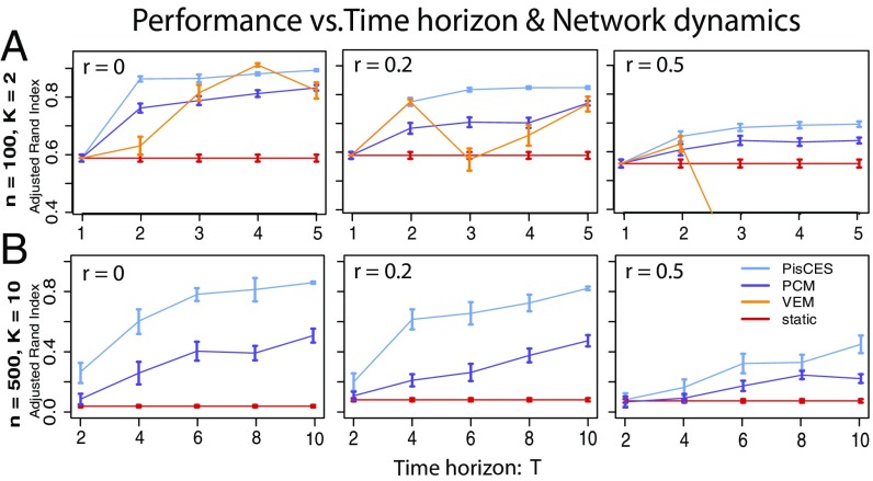
Fig. 1.

Performance on synthetic networks as a function of time horizon and class dynamics, as measured by the adjusted Rand index between true and estimated community labels. Networks were generated under a dynamic DCBM (Eqs. 13–15) with three key parameters: $p_{\text{in}}$ and $p_{\text{out}}$, which determine the in-cluster and out-of-cluster edge probability/density, and $r$, which determines the amount of change in cluster memberships between consecutive networks (0 for no change). For A, $K=2,n=100,p_{\text{in}}=(0.2,0.25),p_{\text{out}}=0.1$, and for B, $K=10,n=500,p_{\text{in}}=(0.2,0.35),p_{\text{out}}=0.1$. Shown are 100 simulations per data point.

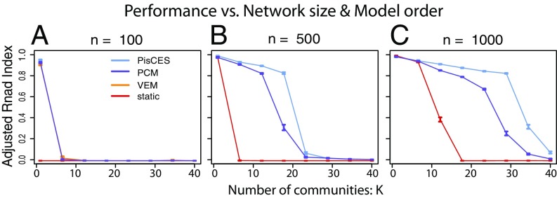
Fig. 2.

Performance on synthetic networks as a function of network size and number of communities, as measured by ARI between true and estimated community labels. (A–C) Networks are generated under the dynamic DCBM with $n\in \{100,500,\mathrm{1,000}\}$, $K\in \{1,4,8,12,\dots ,40\}$, $r=0.1$, $p_{\text{in}}=(0.2,0.5)$, $p_{\text{out}}=0.1$, $T=10$. Shown are 100 simulations per data point.

For comparison, we evaluate a variational–expectation-maximization (“VEM”) likelihood method for the dynamic DCBM (8) and a spectral method [“PCM” (preserving cluster membership)] (17); as a baseline we contrast these with static spectral clustering (“static”). (Due to its computational complexity, results for VEM are shown for n = 100 only, as its runtimes were impractical for $n\ge 500$.)

Fig. 1 shows improving performance for PisCES as the time horizon $T$ increases (which allows greater sharing of information) and decreasing performance as the nodal classes evolve more rapidly over time. Fig. 2 shows increasing performance for all methods as the network size $n$ increases and decreasing performance as the number of nodal classes $K$ increases. In all cases, PisCES performs comparably to or better than the other methods.

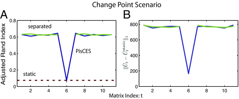
In Methods, we mention that PisCES suppresses the amount of smoothing at times where an outlier or a change point exists in the data. To demonstrate this, Fig. 3 shows the results of a simulation with $T=11$ where the class labels evolve as a dynamic DCBM except at times $t=6$ and $t=7$, at which point they are randomized with no dependence on past time steps. Fig. 3 shows that the estimated ${\overline{U}}_t$ at $t=6$ closely resembles the output of static spectral clustering, while at the other time steps the output closely resembles that of PisCES applied to $A_1,\dots ,A_5$ and to $A_7,\dots ,A_{11}$.

Fig. 3.

Performance of PisCES in a scenario with outlier at time $t=6$ (main text). Simulations were generated from a dynamic DCBM with $n=500$, $K=10$, $p_{\text{in}}=(0.3,0.3)$, $p_{\text{out}}=0.1$, $r=1$ for $A_6$, and $r=0.1$ outside the change point. (A) ARI performance of PisCES applied to $A_1,\dots ,A_{11}$ (blue line), static spectral clustering (static, red dashed line), and PisCES applied separately to $A_1,\dots ,A_5$ and to $A_7,\dots ,A_{11}$ (“separated,” green lines). (B) ${\parallel {\overline{U}}_t-{\overline{U}}_t^{\text{static}}\parallel }_1$, where ${\overline{U}}_t$ is the output of PisCES (green) or “separate” (blue), and ${\overline{U}}_t^{\text{static}}$ is the output of static.

Results

Background.

The transcriptional patterns of the developing primate brain are of keen interest to neuroscientists and others interested in neurological and psychiatric disorders. Bakken et al. (18) provide a high-resolution transcriptional atlas of rhesus monkeys (Macaca mulatta) built from recorded samples of gene expression, including expression of 9,173 genes that can be mapped directly to humans. The samples span six prenatal ages from 40 embryonic days to 120 embryonic days (E40–E120) and four postnatal ages from 0 mo to 48 mo after birth (0 M to 48 M; SI Appendix, section S7). These ages represent key stages of development in the prenatal phase and key milestones postnatally (newborn, juvenile, teen, and mature). The samples can also be divided into different regions of the brain and further into different layers (i.e., subregions) within each region. For example, in postnatal ages, the medial prefrontal cortex region (mPFC) can be divided into contiguous layers L6–L2, with a more complex layer parcellation in prenatal ages (SI Appendix, Table S2).

The changes in gene expression over spatiotemporal periods have been fairly well studied, but changes in coexpression are less well understood. Bakken et al. (18) used weighted gene coexpression network analysis (WGCNA) (29) to identify gene communities in the cortex of rhesus monkeys at each age; roughly speaking, this corresponds to dividing the samples by age, constructing gene coexpression networks from each subset of samples, and then performing a clustering analysis on each network. Our goal is to take this investigation farther using PisCES, but in this present work we give exploratory results only to demonstrate proof of concept.

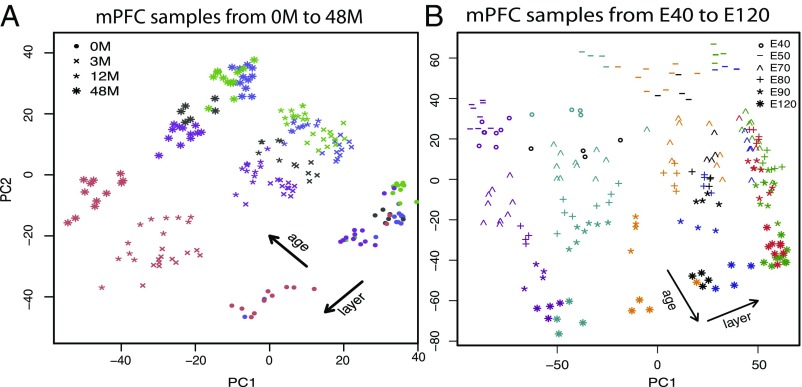
Due to its importance in understanding developmental brain disorders, we focus on the mPFC and use only the $423$ samples corresponding to that region in our analysis (SI Appendix, Fig. S8). For these samples, variability in the first two components of principal components analysis is explained roughly equally by their layer or by their age, suggesting that they may be grouped by either variable (Fig. 4). To illustrate that PisCES can be used over time or location, we choose to divide the $209$ prenatal samples by age category (E40–E120) and divide the $214$ postnatal samples by their layer within the mPFC region (L6–L2).

Fig. 4.

(A and B) Top two principal components for mPFC samples in (A) postnatal ages 0 M to 48 M and (B) prenatal ages E40–E120. Age and layer of each sample are depicted by marker shape and color, respectively. Shown are postnatal layers L2 (blue), L3 (green), L4 (black), L5 (purple), and L6 (red) and prenatal layers VZ (purple), SZ/IFZ (cyan), IZ/OFZ (orange), SP (blue), L5/L6/CPi (green), L2/L3/CPo (red), and MZ (black). Samples obtained from a given age and layer are relatively homogeneous in their rates of transcription.

For each group of samples, coexpression networks (gene networks in which edges encode coexpression level between gene pairs) are constructed by the procedure of refs. 18 and 29. Specifically, adjacency matrix $A_t$ for group $t\in \left(\text{E40–E120, L6–L2}\right)$ is generated by soft thresholding the empirical correlation matrix

$${[A_t]}_{ij}={|\text{corr}(g_i,g_j)|}^6,\hspace{1em}i\ne j,$$ [17]

where $g_i$ and $g_j$ are the recorded expression levels for genes $i$ and $j$ in the samples belonging to group $t$.

PisCES Results.

PisCES—using Eq. S17 for $\delta$—is run separately on the pre- and postnatal samples. The detected communities vary in composition, size, and density (Dataset S1); see SI Appendix, Table S3 for descriptive summaries. For pre- and postnatal analyses we compare the performance of algorithms, using a measure of log-likelihood (SI Appendix, Fig. S9). PisCES generally performs the best across ages and layers, suggesting that the dynamic progression is informative.

To assess the similarity of communities across periods we compute the adjusted Rand index (ARI) (27) between subsequent periods. We find that, for the most part, communities in adjacent ages or layers are more similar in composition than those in noncontiguous periods (SI Appendix, Table S4); for example, we find that communities in E120 are most similar to those in E90 (ARI = 0.23) and least similar to those in E40 (ARI = 0.05).

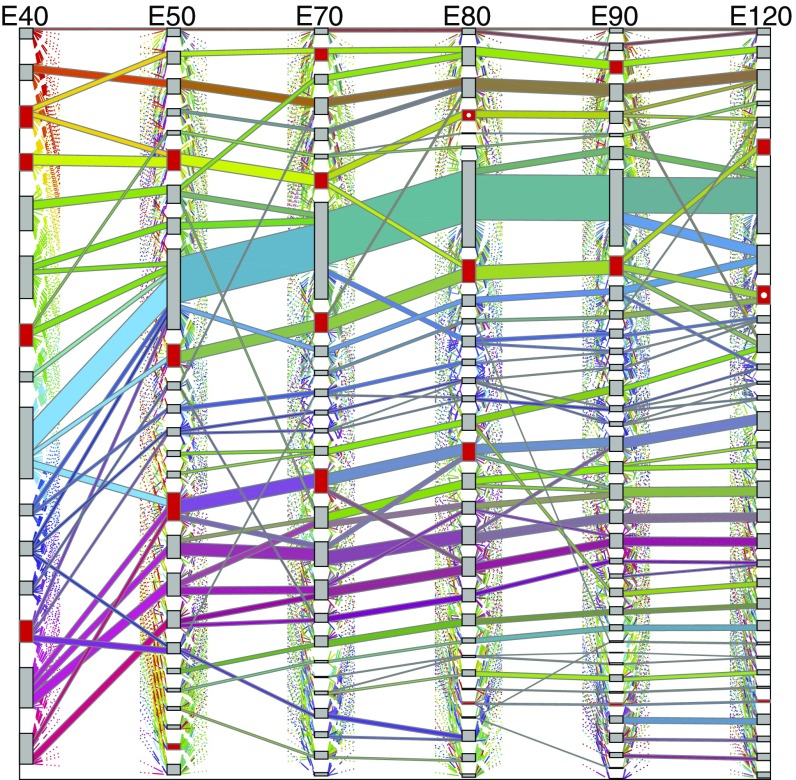
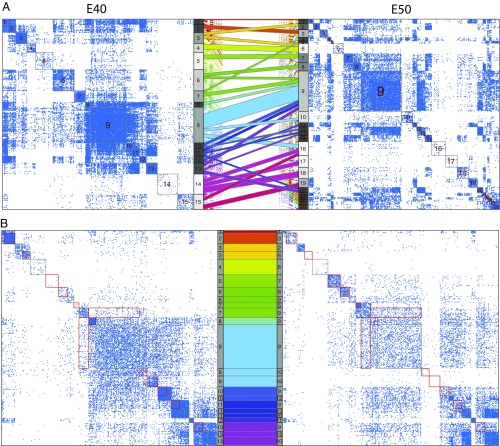
Many communities persist in pre- and postnatal samples as illustrated by the Sankey plots (Fig. 5 and SI Appendix, Fig. S10). To better understand the Sankey display, we focus on the transition from E40 to E50 and display thresholded weighted adjacency matrices along with the mapping between communities (Fig 6A). The ninth community (blue) appears to dominate Fig. 5; however, closer inspection of Fig. 6A suggests that this cluster may be dominated by genes that are connected with many genes outside of the cluster, indicating that this cluster is not likely to be interesting biologically.

Fig. 5.

Sankey plot for prenatal cases. Gray and red boxes denote communities, with height indicating community size. Colored “flows” denote groups of genes moving between communities, with height indicating flow size. To reduce clutter, only large flows ($>100$ genes or $>15\%$ of its source and destination community) are shown; small flows are partially drawn using dotted lines. Each flow’s color is determined by its gene membership and equals the mixture of the colors of its input flows. NPG-enriched communities are denoted by red boxes, with ASD-enriched communities further marked by a white circle (E80, fourth from top, and E120, ninth from top).

Fig. 6.

(A) Sankey plot for stages E40 and E50 only, along with the thresholded Laplacian matrices L_E40 and L_E50 corresponding to those stages. (B) Submatrices of L_E40 and L_E50 corresponding to those genes in large flows between E40 and E50 (excluding E40 communities 14 and 15). To facilitate comparison, the genes in L_E50 have been reordered to match their ordering in L_E40. Red boxes highlight large difference between the submatrices. In both A and B, the flow colors match their coloring in Fig. 5.

To facilitate visual comparison of the adjacency matrices, only those nodes belonging to the major flows between E40 and E50 have been included in Fig. 6B. Cluster boundaries are delineated in red (featured) or gray. The density of some clusters decreases markedly from E40 to E50 (clusters $2\to 3$, $3\to 6$, $9\to 10$, $9\to 16$), while others increase (clusters $5\to 7$, $6\to 8$, $6\to 9$). Genes in dense clusters $7$, $8$, $10$, $11$, and $13$ go to cluster $9$ and lose their tight connectivity as they enter this catch-all cluster, suggesting that some genes act together, but only for brief periods.

For each community, we examine the composition of genes to interpret function using Enrichr (amp.pharm.mssm.edu/Enrichr/) for annotation. Communities are highlighted in red for which neural projection guidance (NPG) genes show significant enrichment (Fig. 5 and SI Appendix, Fig. S10). Given the hypothesis that strongly correlated genes share regulation and/or function (30), we examined the communities to determine whether any are enriched with the Simons Foundation Autism Research Initiative (SFARI) autism spectrum disorder (ASD) risk genes (classes 1, 2, 3, and S) (https://gene.sfari.org/autdb/GS_Home.do). Across prenatal communities we observe the strongest clustering of ASD genes in two communities, one at E80 and another at E120 (white dot in red). Both of these communities are enriched for NPG and synaptic transmission (ST) genes and fall in NPG- and ST-enriched paths (SI Appendix, Fig. S11). NPG and ST genes have been strongly implicated with ASD (31, 32).

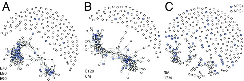
We further investigate the 263 NPG genes that persist in nominally significant enriched communities across at least three consecutive periods (NPG⁺) to identify the properties of the most highly persistent genes. These 64 NPG⁺ genes show a notable pattern of expression across ages and layers in contrast to the other NPG genes (NPG⁻). The former set of genes expresses more highly in mPFC at all ages and layers, but especially during the period just before and at birth (SI Appendix, Fig. S12) A thresholded-correlation network (Fig. 7) shows how the NPG genes coexpress within three epochs of development: E70–E90, E120–0M, and 3M–12M. Clearly the NPG⁺ genes are more tightly clustered at every epoch and there is a notable pattern to the development of clustered genes over time (SI Appendix, Fig. S13). All of these results suggest that a subset of NPG genes plays a strong coordinated role in mid-to-late fetal development in the mPFC, up to and including the time of birth.

Fig. 7.

(A–C) The correlation networks for all NPG genes in different time bands. NPG genes with pairwise correlations at least $0.7$ in the specific time band are connected with edges; nodes for NPG⁺ genes are filled. Fruchterman–Reingold layout (implemented by igraph’s layout_nicely function: igraph.org/r/doc/layout_nicely.html) is applied to illustrate network structures.

ST genes also show strong clustering and persistence in the prenatal analysis; however, unlike NPG genes, the tight clustering of ST genes is not apparent in the postnatal analysis of layers. And yet ST genes become most strongly expressed at birth and continue to be highly expressed throughout life in the mPFC (SI Appendix, Fig. S14A). This seeming contradiction illustrates a limitation of correlation to accurately capture the relationships between genes under certain conditions. Examining the correlation pattern between two ST genes over two periods of time reveals the problem (SI Appendix, Fig. S14B). At E120 the genes have considerable variability in expression and show a strong correlation, but at 0M both genes are expressing at their maximum level. When this happens, there is insufficient variability in expression to detect correlation between genes, and hence the correlation is near zero. This suggests that other measures of coexpression will be needed as we continue to investigate gene communities.

Discussion

Community detection, which involves identification of the number of clusters in a network and the membership of each node, is a challenging problem, especially in applications like gene coexpression when the information about the network is uncertain. This paper aims to improve community detection within networks by incorporating available information about the evolution of a network over time. PisCES works by smoothing the signal contained in a series of adjacency matrices, ordered by time or developmental unit, to permit analysis by spectral clustering methods designed for static networks.

Applying PisCES to the medial prefrontal cortex in rhesus monkey brains from near conception to adulthood reveals communities that persist over numerous developmental periods, communities that merge and diverge over time, and others that are loosely organized and ephemeral. PisCES provides a powerful tool to facilitate the discovery of such fine-scale dynamic structures in coexpression data.

Weighted adjacency matrices derived from gene-coexpression data over a number of time frames or developmental periods are ideal for PisCES. These estimates are usually derived from correlation matrices and are often based on a limited number of samples when the spatial–temporal partitions are extremely fine. But, in this situation, dynamic smoothing across partitions can increase the reliability of the resulting communities.

Estimates of community structure provided by PisCES for the rhesus monkeys have highlighted features that comport with known brain development, such as the coordinated expression of NPG and ST genes. This provides a proof of concept for the analysis paradigm. We posit that in-depth study of gene communities over spatial and temporal partitions of the brain will elucidate key developmental periods and communities associated with neurological disorders.

References

- 1.Kolaczyk ED. Statistical Analysis of Network Data: Methods and Models. 1st Ed Springer; New York: 2009. [Google Scholar]
- 2.Newman M. Networks: An Introduction. Oxford Univ Press; New York: 2010. [Google Scholar]
- 3.Holland PW, Laskey KB, Leinhardt S. Stochastic block models: First steps. Soc Networks. 1983;5:109–137. [Google Scholar]
- 4.Wang YJ, Wong GY. Stochastic blockmodels for directed graphs. J Am Stat Assoc. 1987;82:8–19. [Google Scholar]
- 5.Karrer B, Newman MEJ. Stochastic blockmodels and community structure in networks. Phys Rev E. 2011;83:016107. doi: 10.1103/PhysRevE.83.016107. [DOI] [PubMed] [Google Scholar]
- 6.Rohe K, Chatterjee S, Yu B. Spectral clustering and the high-dimensional stochastic blockmodel. Ann Stat. 2011;39:1878–1915. [Google Scholar]
- 7.Lei J, Rinaldo A. Consistency of spectral clustering in stochastic block models. Ann Stat. 2015;43:215–237. [Google Scholar]
- 8.Matias C, Miele V. Statistical clustering of temporal networks through a dynamic stochastic block model. J R Stat Soc Ser B Stat Methodol. 2016;79:1119–1141. [Google Scholar]
- 9.Ghasemian A, Zhang P, Clauset A, Moore C, Peel L. Detectability thresholds and optimal algorithms for community structure in dynamic networks. Phys Rev X. 2016;6:031005. [Google Scholar]
- 10.Cribben I, Yu Y. Estimating whole-brain dynamics by using spectral clustering. J R Stat Soc Ser C Appl Stat. 2017;66:607–627. [Google Scholar]
- 11.Nguyen NP, Dinh TN, Shen Y, Thai MT. Dynamic social community detection and its applications. PLoS One. 2014;9:e91431. doi: 10.1371/journal.pone.0091431. [DOI] [PMC free article] [PubMed] [Google Scholar]
- 12.Xu KS, Hero AO. Dynamic stochastic blockmodels for time-evolving social networks. IEEE J Selected Top Signal Process. 2014;8:552–562. [Google Scholar]
- 13.Mucha PJ, Richardson T, Macon K, Porter MA, Onnela JP. Community structure in time-dependent, multiscale, and multiplex networks. Science. 2010;328:876–878. doi: 10.1126/science.1184819. [DOI] [PubMed] [Google Scholar]
- 14.Bazzi M, et al. Community detection in temporal multilayer networks, with an application to correlation networks. Multiscale Model Simul. 2016;14:1–41. [Google Scholar]
- 15.Bassett DS, et al. Robust detection of dynamic community structure in networks. Chaos. 2013;23:013142. doi: 10.1063/1.4790830. [DOI] [PMC free article] [PubMed] [Google Scholar]
- 16.Taylor D, Myers SA, Clauset A, Porter MA, Mucha PJ. Eigenvector-based centrality measures for temporal networks. Multiscale Model Simul. 2017;15:537–574. doi: 10.1137/16M1066142. [DOI] [PMC free article] [PubMed] [Google Scholar]
- 17.Chi Y, Song X, Zhou D, Hino K, Tseng BL. Evolutionary spectral clustering by incorporating temporal smoothness. In: Berkhin P, Caruana R, Wu X, editors. Proceedings of the 13th ACM SIGKDD International Conference on Knowledge Discovery and Data Mining. Association for Computing Machinery; New York: 2007. pp. 153–162. [Google Scholar]
- 18.Bakken TE, et al. A comprehensive transcriptional map of primate brain development. Nature. 2016;535:367–375. doi: 10.1038/nature18637. [DOI] [PMC free article] [PubMed] [Google Scholar]
- 19.Amini AA, et al. Pseudo-likelihood methods for community detection in large sparse networks. Ann Stat. 2013;41:2097–2122. [Google Scholar]
- 20.Newman ME. Spectral methods for community detection and graph partitioning. Phys Rev E. 2013;88:042822. doi: 10.1103/PhysRevE.88.042822. [DOI] [PubMed] [Google Scholar]
- 21.Sussman DL, Tang M, Fishkind DE, Priebe CE. A consistent adjacency spectral embedding for stochastic blockmodel graphs. J Am Stat Assoc. 2012;107:1119–1128. [Google Scholar]
- 22.Sarkar P, et al. Role of normalization in spectral clustering for stochastic blockmodels. Ann Stat. 2015;43:962–990. [Google Scholar]
- 23.Chen K, Lei J. Network cross-validation for determining the number of communities in network data. J Am Stat Assoc. 2017 doi: 10.1080/01621459.2016.1246365. [DOI] [Google Scholar]
- 24.Li T, Levina E, Zhu J. 2017. Network cross-validation by edge sampling. arXiv:1612.04717v4.
- 25.Wang YR, et al. Likelihood-based model selection for stochastic block models. Ann Stat. 2017;45:500–528. [Google Scholar]
- 26.Le CM, Levina E. 2015. Estimating the number of communities in networks by spectral methods. arXiv:1507.00827.
- 27.Hubert L, Arabie P. Comparing partitions. J Classif. 1985;2:193–218. [Google Scholar]
- 28.Meilă M. Local equivalences of distances between clusterings—a geometric perspective. Mach Learn. 2012;86:369–389. [Google Scholar]
- 29.Langfelder P, Horvath S. WGCNA: An R package for weighted correlation network analysis. BMC Bioinformatics. 2008;9:559. doi: 10.1186/1471-2105-9-559. [DOI] [PMC free article] [PubMed] [Google Scholar]
- 30.Parikshak N, et al. Integrative functional genomic analyses implicate specific molecular pathways and circuits in autism. Cell. 2013;155:1008–1021. doi: 10.1016/j.cell.2013.10.031. [DOI] [PMC free article] [PubMed] [Google Scholar]
- 31.Willsey AJ, et al. Coexpression networks implicate human midfetal deep cortical projection neurons in the pathogenesis of autism. Cell. 2013;155:997–1007. doi: 10.1016/j.cell.2013.10.020. [DOI] [PMC free article] [PubMed] [Google Scholar]
- 32.De Rubeis S, et al. Synaptic, transcriptional and chromatin genes disrupted in autism. Nature. 2014;515:209–215. doi: 10.1038/nature13772. [DOI] [PMC free article] [PubMed] [Google Scholar]
Associated Data
This section collects any data citations, data availability statements, or supplementary materials included in this article.