Confirmation of a gyral bias in diffusion MRI fiber tractography

Abstract

Diffusion MRI fiber tractography has been increasingly used to map the structural connectivity of the human brain. However, this technique is not without limitations; for example, there is a growing concern over anatomically correlated bias in tractography findings. In this study, we demonstrate that there is a bias for fiber tracking algorithms to terminate preferentially on gyral crowns, rather than the banks of sulci. We investigate this issue by comparing diffusion MRI (dMRI) tractography with equivalent measures made on myelin‐stained histological sections. We begin by investigating the orientation and trajectories of axons near the white matter/gray matter boundary, and the density of axons entering the cortex at different locations along gyral blades. These results are compared with dMRI orientations and tract densities at the same locations, where we find a significant gyral bias in many gyral blades across the brain. This effect is shown for a range of tracking algorithms, both deterministic and probabilistic, and multiple diffusion models, including the diffusion tensor and a high angular resolution diffusion imaging technique. Additionally, the gyral bias occurs for a range of diffusion weightings, and even for very high‐resolution datasets. The bias could significantly affect connectivity results using the current generation of tracking algorithms.

1. INTRODUCTION

It has long been recognized that a detailed map of the structural connections in the brain would be of great value for understanding cognition, brain function, normal development, and aging, as well as neurological disease and disorders (Schmahmann & Pandya, 2009, 2007; Sporns, 2013). Thus, creating a comprehensive description of the neuronal connections in the brain (i.e., the human connectome (Sporns, Tononi, & Kotter, 2005)) has been a major scientific goal for decades (Schmahmann & Pandya, 2007). Early investigators relied on techniques performed on postmortem tissue that limit analysis to small brain areas, or one system of pathways at a time (see Schmahmann & Pandya, 2009, 2007 for historical reviews). The advent of diffusion MRI (dMRI) (Le Bihan et al., 1986) and dMRI fiber tracking (Mori, Crain, Chacko, & van Zijl, 1999) opened up the possibility of studying white matter anatomy on living subjects, and across the entire brain, in a matter of minutes.

The ability to noninvasively study the human brain has made dMRI one of the main tools used in connectomics research for inferring anatomical pathways connecting brain regions. Significant progress has been made in modeling the network architecture of the brain (Hagmann et al., 2008, 2007; Honey et al., 2009), parcellating the cortex into functionally and anatomically distinct subregions (Behrens & Johansen‐Berg, 2005; Mars et al., 2011), and making detailed measurements of white matter microstructure (Dyrby, Sogaard, Hall, Ptito, & Alexander, 2013; Gong et al., 2005; Miller et al., 2011). However, despite its widespread use in inferring the “connectedness” between brain regions, dMRI fiber tracking is not without its limitations (Jones, Knosche, & Turner, 2013).

For an accurate connectivity map of the brain, estimated dMRI fiber trajectories (streamlines) must be able not only to follow major fiber bundles through the deep white matter, but must also correctly follow fibers as they cross the white matter/gray matter (WMGM) boundary. This is particularly problematic in areas of the cerebral cortex that exhibit complex folding and convolutions. Recently, it has been shown that tractography streamlines have a tendency to terminate primarily on gyral crowns, rather than the walls of sulci, or the sulcal fundi (Chen et al., 2013; Kleinnijenhuis et al., 2015; Nie et al., 2012; Reveley et al., 2015). These results could have significant implications regarding cortical development and morphogenesis (Chen et al., 2013; Nie et al., 2012). However, it has been suggested that, rather than an anatomical reality, this likely reflects a bias in fiber tracking algorithms (Van Essen et al., 2014). Clearly, a tendency for streamlines to track toward certain regions of the brain could significantly bias quantitative connectivity studies using dMRI, including network connectome profiles and brain parcellation results.

The observation that tractography streamlines are denser in gyri than in sulci could have several explanations. For one, it could have genuine anatomical underpinnings. Due to their convexity (Peters & Jones, 1984; Van Essen & Maunsell, 1980), the cortical volume (per unit surface area of the WMGM boundary) at gyral crowns would be greater than at the relatively flat sulcal walls or concave fundi (Van Essen et al., 2014). If the axonal density associated with a unit volume of the cortex were to be relatively homogenous, as is often assumed (Donahue et al., 2016; Rockel, Hiorns, & Powell, 1980; Van Essen et al., 2014), this would imply that the number of axons crossing the WMGM boundary at the gyral crowns would have to be higher than those along the banks or fundus of sulci (Van Essen et al., 2014).

On the other hand, the “gyral bias” could be an artifact of tracking algorithms, due either to technical limitations or inherent simplifying assumptions. Analysis of myelin‐stained sections has shown that many fibers follow a sharply curved trajectory as they enter the cortex, particularly those near the sulcal walls (Budde & Annese, 2013; Sotiropoulos et al., 2013a; Van Essen et al., 2014). Because of the large voxel size of dMRI acquisitions (typically 2–3 mm), these areas are prone to partial volume effects. This could bias orientation estimates along the WMGM border to point in the direction of the adjacent white matter (which is often tangential to the boundary (McNab et al., 2013; Van Essen et al., 2014)), rather than correctly pointing toward the sulcal cortical surface (Van Essen et al., 2014). Because these orientation estimates form the input of most tracking algorithms, any fiber tracking would subsequently exhibit a bias.

Even if fiber orientations were estimated perfectly, tracking algorithms might still not be able to propagate correctly into the cortex. Tracking usually involves choosing a curvature threshold, a maximum angle that the trajectory is able to turn through over a certain distance (Jones et al., 2013). This parameter is often justified on the basis that fibers in the brain typically do not exhibit sharp bends; however, this will clearly preclude accurately tracking fibers that truly exhibit curvatures greater than this threshold. Similarly, in voxels where multiple “crossing” fibers are detected, many algorithms will propagate in the direction with the least angular deviation from the previous tracking step. Again, along the cortex, this could lead to streamlines continuing to follow the direction of the white matter bundles, rather than exiting the white matter to enter the cortex (Van Essen et al., 2014), even if these fibers were correctly detected.

In addition to limitations of the dMRI acquisition and tracking algorithm, bias can be introduced in part by the strategy used to begin streamline propagation. Some of the most common seeding strategies include propagating streamlines from every voxel in the brain (“whole brain” seeding), or seeding from every voxel in the white matter (“white matter” seeding). Because longer white matter pathways occupy a greater volume from which to seed, these pathways tend to be over‐represented in streamline reconstruction (Smith, Tournier, Calamante, & Connelly, 2013; Yeh, Smith, Liang, Calamante, & Connelly, 2016). If these pathways were to terminate more frequently in specific regions (i.e., gyral crowns), this could, again, lead to a larger number of streamlines entering this area. To compensate for this, it is common in many brain network studies to heuristically scale the contribution of each streamline to the overall connection density by the reciprocal of the streamline length (Hagmann et al., 2010, 2008). Several groups have attempted to bypass this potential source of bias by seeding only from the WMGM boundary (Girard, Whittingstall, Deriche, & Descoteaux, 2014; Smith, Tournier, Calamante, & Connelly, 2012). However, it is unclear what effect the seeding strategy, and subsequent quantification, have on potential gyral biases in diffusion tractography.

Taken together, it is clear that dMRI tractography has limitations that could produce significant bias in certain anatomical regions, and prevent creation of accurate connectivity maps of the brain. Hence, there is a need to better understand to what extent, and under which circumstances, these biases occur.

In this study, using histology as a validation tool, we compared dMRI fiber tractography to myelin histology performed on a Rhesus macaque brain to investigate gyral bias. We first asked how the true (histologically defined) density of fibers entering the cortex varies along the gyral blade, and if this “fiber density profile” varies between different gyri. Next, we asked whether fiber tracking using the very commonly used diffusion tensor imaging (DTI) model is biased toward the gyral crowns, relative to histological measurements, and if this bias is dependent on seeding or fiber quantification strategies. We then investigated the axonal trajectories near the WMGM boundary along gyral blades by assessing fiber curvature, the effects of the tractography curvature threshold, and the agreement with dMRI estimated fiber orientations. We then assess whether the b‐value, or diffusion‐weighting, affects the results in any way. In addition, intuition suggests that increasing the spatial resolution of dMRI images would lead to more accurate fiber tracking (Heidemann, Anwander, Feiweier, Knosche, & Turner, 2012; Van Essen et al., 2014) and a reduced gyral bias. Hence, we analyze different tractography methods using data‐sets acquired at varying spatial resolutions to test this hypothesis. Finally, we then move away from the commonly used diffusion tensor and assess tractography based on a higher order algorithm (constrained spherical deconvolution (Tournier, Calamante, & Connelly, 2007)) for estimating fiber orientation, and use this to construct 3D fiber pathways.

2. METHODS

2.1. MRI acquisition

All animal procedures were approved by the Vanderbilt University Animal Care and Use Committee. MRI experiments were performed on a single hemisphere of an adult Rhesus macaque (Macaca Mulatta) brain that had been perfused with physiological saline followed by 4% paraformaldehyde. The brain was then immersed for 3 weeks in phosphate‐buffered saline (PBS) medium with 1 mM Gd‐DTPA in order to reduce longitudinal relaxation time (D'Arceuil, Westmoreland, & de Crespigny, 2007). The brain was placed in liquid Fomblin (California Vacuum Technology, CA) and scanned on a Varian 9.4 T, 21 cm bore magnet. A structural image was acquired using a 3D gradient echo sequence (TR = 50 ms; TE = 3 ms; flip angle = 45°) at 200 μm isotropic resolution.

Diffusion data were then acquired with a 3D spin‐echo diffusion‐weighted EPI sequence (TR = 340 ms; TE = 40 ms; NSHOTS = 4; NEX = 1; Partial Fourier k‐space coverage = .75) at 400 μm isotropic resolution. Diffusion gradient pulse duration and separation were 8 ms and 22 ms, respectively, and the b‐value was set to 6,000 s/mm². This value was chosen due to the decreased diffusivity of ex vivo tissue, which is approximately a third of that in vivo (Dyrby et al., 2011), and is expected to closely replicate the signal attenuation profile for in vivo tissue with a b‐value of ∼2,000 s/mm². A gradient table of 101 uniformly distributed directions (Caruyer, Lenglet, Sapiro, & Deriche, 2013) was used to acquired 101 diffusion‐weighted volumes with four additional image volumes collected at b = 0. Unless otherwise noted, all fiber tractography was performed on this dataset.

To assess the effects of the diffusion weighting on any potential gyral bias, the full diffusion acquisition was repeated with b‐values of 3,000, 9,000, and 12,000 s/mm², while keeping all other acquisition parameters (including diffusion times) constant. Higher b‐values have been shown to be beneficial for several advanced diffusion (and fiber) reconstruction algorithms (Alexander & Barker, 2005; Dyrby et al., 2011; Tournier, Calamante, & Connelly, 2013). Finally, to assess the effects of image resolution, the full acquisition was repeated with resolution ranging from 300 μm isotropic to 800 μm isotropic, in 100 μm increments. Here, all b‐values were set to 6,000 s/mm². Again, all acquisition parameters were kept constant (including diffusion times), except for field‐of‐view and number of phase‐encoding and readout points required to achieve the intended resolution.

The signal‐to‐noise ratio in the white matter of the non‐diffusion weighted images ranged from ∼36 in the 300 μm isotropic images to ∼310 in the 800 μm isotropic images, values much higher than those typical of diffusion MRI on clinical scanners (∼16–20). Comparing the macaque and human brain based on volume only (∼80 and 1200 mL (Allen, Damasio, & Grabowski, 2002), respectively), our 300 μm isotropic voxels would be roughly equivalent to ∼740 μm isotropic in the human, while our 800 μm isotropic scans would resemble human voxels at ∼2 mm isotropic.

2.2. Histology

After imaging, the brain was embedded in dry ice and sectioned on a microtome at a thickness of 25 μm in the coronal plane. Using a Canon EOS20D (Lake Success, NY, USA) digital camera, the tissue block was digitally photographed prior to cutting every twelfth section, resulting in a through‐plane photographic resolution of 300 um. Thirty five slices, with an effective slice gap of 1.8 mm, were selected for this study. The tissue sections were then stained for myelin using the silver staining method of Gallyas (Gallyas, 1971) and mounted on glass slides. Whole‐slide bright‐field microscopy was performed using a Leica SCN400 Slide Scanner at 20× magnification, resulting in an in‐plane resolution of 0.5 μm/pixel.

2.3. Registration

To transfer the MRI information into high‐resolution histological space (or vice‐versa), a multistep registration procedure was used (Choe et al., 2011). Briefly, each 2D histological slice was registered to the corresponding block‐face image using a mutual information based 2D linear registration followed by 2D nonlinear registration using the adaptive bases algorithm (ABA)(Rohde, Aldroubi, & Dawant, 2003). Next, all block‐face photographs were assembled into a 3D block volume, which was registered to the mean MRI b = 0 image using a 3D affine transformation followed by 3D nonlinear registration with ABA. The block to MRI registration was performed for all MRI acquisitions separately. Concatenation of these two deformation fields allows any scalar MRI information (i.e., labels for the crown and walls) to be transformed into histological space. For orientation information derived from MRI, the data were transformed and reoriented appropriately using the preservation of principal directions (PPD) strategy (Alexander & Barker, 2005).

2.4. Data processing

From the histological and MRI datasets, six pieces of information were obtained (Figure 1).

Figure 1.

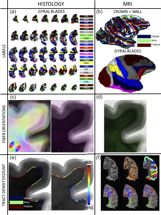
Data processing pipeline. From the histological (left column) and MRI (right column) datasets, six pieces of information are extracted. Twenty‐four gyral blades are manually defined on histological slices (a), while labels for the crown, walls, and fundi are defined based on convexity measures from 3D MRI data (b). The 3D WMGM surface colored with the crown/wall/fundus labels are shown on top, while the gyral labels transferred to MRI space are shown below (note color scheme is same from part 1). Structure tensor analysis (c, left) is used to extract the myelinated, or ground truth, axon orientations (c, right), for comparisons with dMRI estimated fiber orientations (d) after transformation to histological space. A count of axons entering the cortex is made along the entire gyral blade, in gyral crowns and sulcal walls (left) for the myelinated tract density measurement (right) (e), for comparisons with the dMRI tractography connectivity and fiber density measures (f). Shown on top are a select slice from the b0 image, the WMGM boundary, and gyral labels segmented into crowns, walls, and fundi. On bottom are shown results from various tractography algorithms (from left to right: DTI, M1; DTI, M2; CSD, M1) [Color figure can be viewed at http://wileyonlinelibrary.com]

2.4.1. Definition of gyral blades

Gyral blades were defined on the histological sections. Manual labeling of 24 gyral blades across all slices (Figure 1a) was performed by a neuroanatomist (IS), with the help of existing macaque atlases (Bakker, Tiesinga, & Kotter, 2015; Paxinos, Huang, & Toga, 2000). Each gyral region of interest was represented on a minimum of 4 slices, and all described procedures were performed for all regions on all slices.

Gyral blades and abbreviations are as follows: superior frontal gyrus (SFG); medial frontal gyrus (MFG); inferior frontal gyrus (IFG); frontal orbital gyrus (FOG); lateral orbital gyrus (LorG); medial orbital gyrus (MorG); gyrus rectus (Gre); anterior cingulate gyrus (ACgG); precentral gyrus (PrG); superior temporal gyrus (STG); insula (INS); middle temporal gyrus (MTG); inferior temporal gyrus (ITG); postcentral gyrus(PoG); posterior cingulate gyrus (PCgG); supramarginal gyrus (SMG); fusiform gyrus (FuG); posterior parahippocampal gyrus (PPhG); superior parietal lobule (SPL); angular gyrus (AnG); inferior occipital gyrus (IOG); lingual gyrus (LiG); cuneus (CUN); occipital gyrus (OG). Note that one gyrus, PPhG, was removed from analysis as it was determined to be defined only on gyral crowns (see Section 2.4.2), and had no data from sulcal walls for comparison.

The gyral labels were transferred to MRI space (Figure 1b, bottom) using the transformations described above (see Section 2.3). Transferred labels were visually inspected, and manually corrected as necessary.

2.4.2. Defining gyral crowns and sulcal walls

Labels for gyral crowns and sulcal walls were defined from the structural MRI data. Taking advantage of the 3D architecture provided from MRI, many groups have developed methods to reconstruct gyral and sulcal parcellations using mesh‐based, or surface‐based, analysis derived from either mean curvature or convexity measures (Dale, Fischl, & Sereno, 1999; Desikan et al., 2006; Destrieux, Fischl, Dale, & Halgren, 2010; Fischl, Sereno, & Dale, 1999; Fischl et al., 2004; Li, Guo, Nie, & Liu, 2009; Li et al., 2010). Traditionally, the crown of the gyrus is defined by its convexity (negative curvature) (Fischl et al., 2004; Peters & Jones, 1984). The sulcal walls, or banks of the sulci, are the areas of cortex along opposing sides of adjacent gyri (Peters & Jones, 1984) and are characterized by a low curvature (Fischl et al., 2004). Finally, the fundus describes the deepest part of the sulcus (Peters & Jones, 1984) and are regions with positive curvature (Fischl et al., 2004). In this study, we began with a joint segmentation and bias field correction based on integrated local intensity clustering (Li et al., 2008) to create a white matter mask. Next, a mesh of the WMGM boundary was created, and for every vertex, the mean curvature (Dale et al., 1999; Fischl et al., 1999) is calculated. Then, a simple threshold was applied at the 33rd and 66th percentile of the mean curvatures to segment the surface into crown, walls, and fundi (Figure 1b, top). After registration, the labels derived from 3D MRI data were transferred into 2D histological space (Figure 1b, bottom). At this point, we have labels for gyral blades defined in both histolgical and MRI space, and each blade is segmented into crown(s), wall(s), and fundus (fundi).

2.4.3. Myelinated fiber orientations

The ground truth fiber orientations were defined on histological myelin‐stained slices using structure tensor (ST) analysis (Bigun & Granlund, 1987). The ST has been employed on histological sections in 2D on rat (Budde & Frank, 2012) and human (Budde & Annese, 2013; Ronen et al., 2014) brains, and in 3D on macaque (Khan et al., 2015) and squirrel monkey (Schilling et al., 2016) brains. ST analysis is a technique based on the dyadic product of the image gradient vector with itself, and results in an orientation estimate for every pixel in the image (Figure 1c, left). Downsampling of the high‐resolution orientation estimates was employed to determine the primary fiber orientation in 150 μm² areas (Figure 1c, right). These were then used for comparison with the primary orientation estimated from MRI using the diffusion tensor model (see Section 2.4.4), and for analysis of fiber curvature along the WMGM boundary. For visualization, ST values of orientation, anisotropy, and staining intensity are displayed as hue, saturation, and brightness (HSB) images (Figure 1c, left), respectively, at native resolution (Budde & Frank, 2012).

2.4.4. dMRI estimated fiber orientations

We chose to use the tensor model for comparisons of orientation with histology (although any local reconstruction algorithm can be processed and compared in a similar way). The tensor was estimated using a NLLS DT fit (Jones & Basser, 2004). After transformation to and reorientation in histological space (see Section 2.3), the primary eigenvector of the diffusion tensor was projected onto the 2D histological plane (Choe, Stepniewska, Colvin, Ding, & Anderson, 2012; Figure 1d). This 2D projection was then compared to the histological fiber orientations estimated using ST analysis.

2.4.5. Myelinated “tract density”

An automatic count of the axons leaving the white matter and entering the cortex was made along the entire WMGM boundary mesh surface for every gyral blade (Figure 1e). This was performed by dilating the WMGM boundary 50 μm into the cortex (to ensure we were not counting axons in the white matter) and taking the intensity profile along this band. Because the myelinated axons appear as low intensities, the intensity values were inverted, and a count of the number of peaks meeting an (empirically derived) intensity threshold was made. This threshold was kept constant across the entire slice, and for all slices. The fiber density was then the average axon count over a specific distance. For each gyral blade, this measurement was summarized by taking the ratio of the average fiber density at the crown(s) over the average fiber density at the wall(s). We refer to this quantity as the “connectivity profile” of each gyral blade. For statistical analysis, we took the natural log of this ratio. This makes the ratios additive, the variance homogenous, and the distribution symmetric (Aitchison, 1986), which allows for standard parametric hypothesis testing. A positive log‐ratio (ratio > 1) suggests higher fiber connectivity at the crown(s), while a negative value (ratio < 1) suggests higher connectivity at the wall(s).

2.4.6. Diffusion MRI tract density

We begin our study by choosing fiber tractography based on (arguably) the most commonly used local reconstruction technique, diffusion tensor imaging (Basser, Mattiello, & LeBihan, 1994a, 1994b). Three tracking strategies that are ubiquitous in the field are employed, distinguished largely by the strategy for seeding streamlines. Each method is performed using both deterministic and probabilistic propagation techniques. Finally, for each method, four connectivity “scaling” measures are performed.

Method 1 (M1) is based on whole‐brain seeding. This means seeds are initiated from all voxels in the brain, and terminate only when they exit the brain, or exceed the maximum curvature threshold. This method is consistent with analysis based on tract‐density imaging (Calamante, Tournier, Jackson, & Connelly, 2010), and most commonly applied in studies where whole‐brain seeding is used in combination with waypoints to select specified white matter pathways (Knosche, Anwander, Liptrot, & Dyrby, 2015; Yeatman, Dougherty, Myall, Wandell, & Feldman, 2012). For each region of interest (i.e., the crowns and walls for each gyral blade), the number of streamlines ending within the region volume are counted. Method 2 (M2) is seeded throughout the white matter. White matter seeding is the most common strategy for studies mapping the human connectome (Clayden, 2013; Hagmann et al., 2007; Parker et al., 2014), and again, is also commonly performed before addition of inclusion/exclusion masks for extracting specific fiber pathways. For M2, tracking is stopped once the voxel leaves the WM (crosses the WMGM boundary), and the number of pathways terminating on the surface of each label is counted. Method 3 (M3) then seeds from the interface of the WMGM boundary. The method has been proposed as a way to bypass potential seeding biases (Girard et al., 2014; Smith et al., 2012), and is gaining in popularity in structural connectivity pipelines. Again, tracking is terminated when the pathway crosses the WMGM boundary, and the number of pathways terminating on the surface of each label is counted. In all cases, tracking was performed using the publically available software package MRTrix3 (Basser, Pajevic, Pierpaoli, Duda, & Aldroubi, 2000; Tournier, Calamante, & Connelly, 2012), and seeding was repeated until 2,500,000 streamlines were created. Streamlines that did not meet the minimum length criteria of 5× the voxel size were discarded.

The four connectivity scaling measures are as follows. The first option is no normalization at all. This number then represents the raw “count” of streamlines entering each region of interest. The second scaling mechanism is to scale the contribution of each streamline to the total count by the reciprocal of its length. As described above, this is intended to compensate for biases introduced by homogenous seeding throughout the brain, which leads to over‐representation of the long fiber pathways. Third, the number of streamlines can be scaled by the reciprocal of the total node volume. This is intended to compensate for the fact that larger target regions are more likely to be intersected by an overall greater number of streamlines. The results are traditionally interpreted as a connection density (count per volume), which is more of an analogue to our histological measurements (fiber density). (Note that, for M2 and M3, the data are normalized by GMWM surface area, rather than volume.) The final scaling option we assess is to scale the contribution of each streamline by the streamline length (exactly the inverse of the second normalization mechanism). Although not as commonly used in literature, this scaling could be justified on the basis that longer connections are harder to reconstruct than shorter ones due to tract dispersion (uncertainty) and tract deviation (errors in orientating estimation) (Anderson, 2001; Chang, Koay, Pierpaoli, & Basser, 2007; Lazar & Alexander, 2003). Thus, this scaling would emphasize these longer, harder to reconstruct connections as an attempt to correct for the path‐length dependency inherent in fiber tractography (Donahue et al., 2016; Liptrot, Sidaros, & Dyrby, 2014).

To assess the effects of curvature criteria on DTI tracking, tractography was performed with no stopping criteria other than curvature threshold, or leaving the brain mask. The curvature thresholds chosen for analysis were 15°, 30°, 45°, 60°, 75°, 90°, 135°, and 180° (equivalent to no stopping criterion). Similarly, the effect of b‐value and resolution were assessed by performing repeating tractography for all b‐values (3,000–12,000 s/mm²) and for the entire range of resolutions (300–800 μm isotropic). In order to eliminate the effects of the step size on analysis of acquisition resolution, the step size was fixed for all tracking algorithms, at all resolutions, to 10% of the smallest voxel size (i.e., 30 μm step size). Finally, to test tracking biases using a reconstruction method capable of resolving multiple fiber populations, we have chosen a commonly used higher order algorithm, constrained spherical deconvolution (CSD) (Smith et al., 2012), implemented in MRTrix3.

Figure 1f shows the WMGM boundary used for seeding and stopping, the gyral blades segmented into crowns, walls, and fundi, and 3 representative tractograms.

3. RESULTS

3.1. Histological density profile

The results of histological analysis are shown in Figure 2. We find that many gyral crowns do have more dense connectivity than neighboring sulcal walls. Eleven of the 23 regions of interest have a significantly higher fiber count at the crowns, and all but one have a higher average fiber count at the crown (one‐sample t test; p < .05). Across all gyri, we find an overall log‐ratio value of 0.12 (average ratio of 1.13) suggesting an average 13% increased fiber density at the crowns relative to walls. Finally, a 1‐way ANOVA with the gyral blades as factors suggests that the histological fiber density profile is not the same across all gyri (F = 3.27, p < .001).

Figure 2.

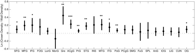
Histological density profile across 23 gyral blades. Average log‐ratio (circles) and 95% confidence intervals (lines) are shown for each region of interest. The value of 0 (ratio = 1) is shown as a horizontal dotted line. Asterisks indicate that log‐ratio is significantly >0 (*p < .05; **p < .01; ***p < .001), which means the gyral crown has significantly higher density than neighboring sulcal wall(s)

3.2. DTI tractography

Figure 3 shows the tractography‐derived fiber density profiles (ratio of crown measure to wall measure) for all gyral blades. Results are shown for all 3 seeding methods, each with both deterministic and probabilistic propagation, and with 4 scaling methods applied to each. It is clear that DTI streamlines are biased toward the gyral crown relative to histology in many gyral blades, for all 3 tracking strategies. No combination of seeding method and quantification is consistently non‐biased across all gyral blades. In fact, many gyral blades show a bias of as much as much as 12× more “connectivity” at crowns that at the corresponding walls.

Figure 3.

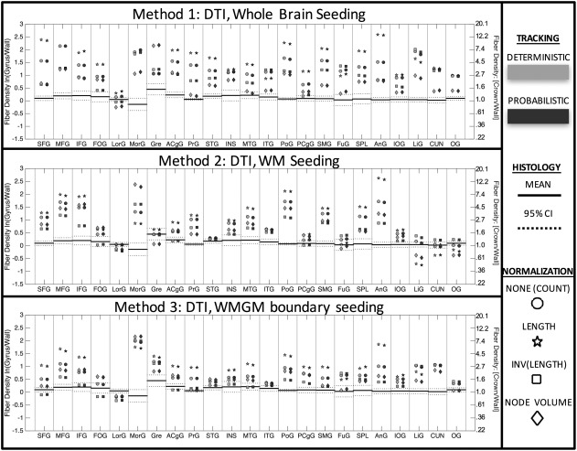
DTI streamlines are biased toward gyral crowns in many gyral blades, for all tracking strategies. The ground truth density profile is shown as horizontal lines (mean ± 95% confidence interval). DTI tractography‐derived densities for whole‐brain seeding (top), white matter seeding (middle), and WMGM boundary seeding (bottom) are shown for each gyral blade, for both deterministic (light gray) and probabilistic (dark gray) propagation. Data are shown as (1) no normalization (circle), normalized by length (star), inverse length (square), and inverse node volume (diamond). Log‐ratio scale is shown on left vertical axis, while the ratio measure is shown on the right. A tractography‐derived value greater than the histological range indicates a bias toward the gyral crowns

Condensing this information across all gyri (Figure 4) shows that across the whole brain, all algorithms are significantly biased relative to histology, and consistently overestimate connectivity at the gyral crowns by a factor of between 1.5 and 5. Several trends are apparent. First, bias is dependent on seeding method (p < .001, F = 17.64, df = 5), for example, M1 (whole‐brain seeding) has significantly higher bias than M2 and M3. Second, there is no significant difference between deterministic and probabilistic DTI tractography. Finally, there are significant effects of scaling mechanism on the gyral bias (p < .001, F = 27.89, df = 5). For all cases, scaling by length leads to the largest bias, followed by no normalization, then inverse length and inverse node volume. It is important to point out that the methods resulting in a fiber profile most similar to histology—M3 with scaling by inverse length—has no biological, anatomical, or technical basis for scaling by inverse length. This scaling mechanism is tailored to address biases inherent to homogenous white matter seeding, which is not performed in M3. Thus, this combination of seeding and quantification is unlikely to be performed in literature.

Figure 4.

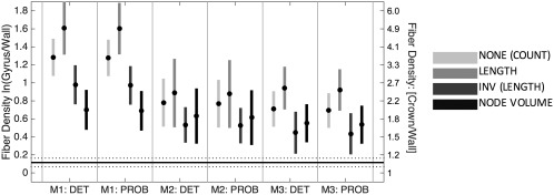
DTI streamlines are denser in gyri than sulci for all three seeding strategies, regardless of subsequent fiber quantification. Mean (circle) and 95% confidence intervals (vertical line) are shown over all gyri for each DTI tracking algorithm. Four quantification strategies include (1) no scaling, (2) scaling by length (3) inverse streamline length, and (4) inverse node volume. Histological mean and 95% confidence intervals across all gyri are shown as horizontal solid and dotted lines

Inspection of the resulting fiber pathways gives insight into potential sources of the bias. Figure 5 shows a select coronal slice, with labels for the crown and walls highlighted. For M1, the most striking feature is the densely populated gray matter in the crown, with sparse fibers throughout the wall. Even more striking, there are areas of the fundus (dotted arrow), where no fibers are able to propagate, a characteristic described in (Reveley et al., 2015), and attributed to the superficial U‐shaped fibers just beneath the infragranular layers of the cortex. In addition, we see relatively sharp curvature into the cortex at the walls (solid arrow), a feature similar to that described in histological sections (Budde & Annese, 2013; Sotiropoulos et al., 2013a; Van Essen et al., 2014). This motivates an analysis of the effect of curvature threshold on tractography results (described later). M2 shows features similar to M1. As in M1, it is clear there is an over‐representation of some of the longer pathways which tend to orient toward the gyral crown. For example, seeding anywhere in the oval leads to an excessively dense representation of tracts in the stalk of the gyrus, which all terminate in the same vicinity.

Figure 5.

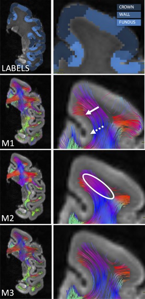
Subset of DTI streamlines for each tracking strategy. Labels for crown, wall, and fundi are shown with a zoomed in view of the SFG. DTI streamlines are shown for M1 (whole brain seeding), M2 (WM seeding), and M3 (WMGM boundary seeding), and are colored based on streamline orientation. The dashed arrow highlights a fundus, where no streamlines are able to propagate. The solid arrow points toward the increased curvature of streamlines entering the GM. And the oval highlights a large, homogenous, area of WM, where seeding will contribute to over‐representation of fibers terminating at the crown [Color figure can be viewed at http://wileyonlinelibrary.com]

To confirm that the dominant source of bias comes from the longer fibers, we separate streamlines by length into short, medium, and long fibers (binned by 33rd and 66th percentiles), and repeat the analysis. Figure 6 shows the results (without scaling), for all algorithms. In all cases, the longer fibers are more biased toward the crowns than medium and short fibers. In agreement with known anatomy (Schmahmann & Pandya, 2009), the short streamlines consist of the short association fibers (U‐fibers) connecting the same or adjacent gyri, while the medium and long fibers are composed of the long association fibers (connectivity of different lobes) and commissural fibers. However, unlike the results of anterograde and retrograde tracer studies (Schmahmann & Pandya, 2009), there is a clear penchant for the association and commissural streamlines to terminate on the gyral crowns. Despite the fact that increased seeding in longer pathways is the dominant source of bias, applying inverse‐length scaling does not eliminate the bias (Figure 6).

Figure 6.

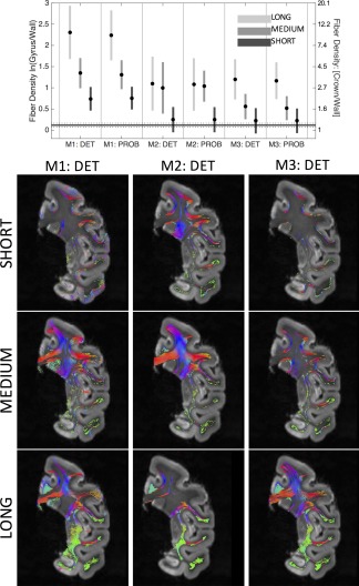
The effects of fiber length on gyral bias. The (unscaled) fiber‐density profile across all gyral blades is shown for long, medium, and short fibers (top). A subset of long, medium, and short fibers is shown for each of the three tracking strategies for a select coronal slice (bottom) [Color figure can be viewed at http://wileyonlinelibrary.com]

3.3. Fiber curvature at the cortex

Two examples highlighting a potential anatomical cause of this bias are shown in Figure 7. Here, we focus on the curvature of fibers as they enter the cortex, taking as examples a slice showing the SFG (a–c) and a slice containing the IFG and FOG areas (d–f). Figures a and d show the WMGM boundary (blue voxels) along the gyral blades and the normal to the boundary (yellow sticks). ST analysis, along with the HSB images, qualitatively highlights the high curvature of fibers entering the cortex along the sulcal wall (b and e), and the relatively low curvature at the crown (c and f).

Figure 7.

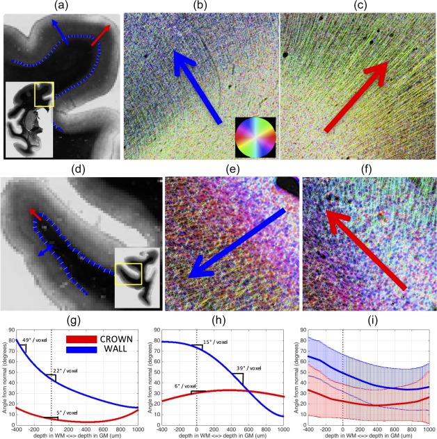
Fibers typically curve more at the sulcal wall than they do at gyral crowns. A histological slice containing the SFG (a) is shown, along with the WMGM border (blue) and the normal to the border (yellow lines). Arrows are shown at the wall (blue) and crown (red) going from white matter into gray matter. Both arrows are perpendicular to the WMGM boundary. High‐resolution HSB images in the same places at the wall b) and crown (c) demonstrate the high curvature of fibers entering the cortex at the walls (b) and the long, straight fibers at the crown (c). A myelin‐stained slice containing IFG and FOG regions (d), and high‐resolution HSB images at the wall (e) and crown (f), show similar trends. The fibers from (a) to (c) are tracked from white matter, into gray matter, and the angle these fibers make with the normal to the WMGM border is recorded (g) for the wall (blue) and crown (red). The slope of this curvature is marked in various locations. The fibers from (d) to (f) are similarly tracked, and the angle at these locations from the wall (blue) and crown (red) are plotted (h). Finally, the results from all gyral blades analyzed (i) are shown for the crown (red) and wall (blue) with the mean (solid line) and standard deviations (vertical lines) plotted for each [Color figure can be viewed at http://wileyonlinelibrary.com]

To quantify the fiber curvature (g and h), the angle the fibers make relative to the normal to the WMGM boundary is plotted as they traverse from white (negative distance) into gray matter (positive distance). In these regions, fibers at the crown stay relatively parallel to the normal (red arrows) throughout the entire path, and are curving at only 5° and 6° per 400 μm as they enter the cortex. At the wall, the fibers bend from nearly perpendicular to the normal, to almost parallel, within a distance of <1.5 mm. In these specific slices, the wall of the SFG (g) is curving at a larger 22°/400 μm entering the cortex, while the highest curvature happens just inside the white matter at nearly 49°/400 μm. For the wall of the IFG and FOG (h), the highest curvature takes place about 400 μm into the cortex, curving at ∼39°/voxel. Thus, in these two examples, the fibers curve more at the sulcal walls than they do at gyral crowns.

While these examples highlight two slices with high curvature at the walls, there is high variability across slices and across gyral blades. Figure 7i shows the mean and standard deviation of the angle relative to the WMGM normal across all analyzed gyral blades. Despite the wide range, two trends are apparent. Fibers at the crown enter the cortex at a smaller angle (relative to the WMGM normal) than those at the walls (22° ± 15° and 50° ± 17°, respectively), and curve less upon entering the cortex than those at the walls.

3.4. Effects of curvature threshold

We next test the effects of curvature threshold on the gyral bias, by performing tractography with varying curvature thresholds (Supporting Information, Figure 1). We find that for all 3 methods, with all 4 quantification techniques, there is no significant effect of pathway curvature threshold on the bias (F ranged from 0.50–0.81, p > .05).

3.5. Angular agreement between histology and dMRI

To assess whether the diffusion orientation estimates are biased toward the gyral crowns relative to the true fiber orientations, we compared the primary diffusion directions (projected onto the 2D histological plane) with the histological fiber orientations estimated using ST analysis (calculated in the 2D plane). Figure 8 (top) shows the angular differences for all voxels along the WMGM boundary, in each of the gyral blades. A positive angular difference indicates that the fiber orientation from diffusion is angled more toward the apex of the gyral blade (relative to ST orientation), while a negative angular difference means it is angled away from the apex. The first, second (median), and third quartiles of this dataset are −8.6°, 2.2°, and 13.7°, respectively. This indicates a slight bias for estimated fiber orientations, the inputs for fiber tracking algorithms, to be oriented slightly more toward the crown than they should be. However, as the tensors become more isotropic, particularly near the cortex, the ambiguity in fiber orientation increases, and could account for much of the angular differences measured.

Figure 8.

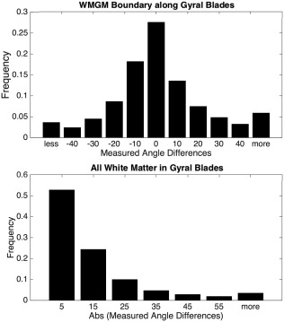
Histograms of measured angle differences. The differences between the true fiber orientation measured with high‐resolution micrographs and the fiber orientation estimated from diffusion imaging are shown for both the voxels comprising the WMGM boundary (top), and those that are in pure WM (bottom). The top figure shows both positive and negative angular differences along the WMGM border, indicating estimated orientation error toward and away from the gyral crown, respectively. The bottom figure shows the absolute value of angular differences in white matter regions contained within the gyral blades

Figure 8 (bottom) shows the absolute angular deviation of voxels in the white matter (this does not include all white matter, only that which is contained within the gyral stalks). The median absolute angular difference in the white matter is 9.2°, indicating that, on average, the tensors differ from the true fiber orientation by <10°, a value in good agreement with previous histological validation studies (Choe et al., 2012; Leergaard et al., 2010).

3.6. Effect of b‐value

Next, DTI tractography was repeated for all acquired b‐values (Supporting Information, Figure 2). For all methods, and all quantification strategies, the diffusion weighting did not have a significant effect on the gyral bias (F ranged from 0.02–0.33, p > .05).

3.7. Effect of image resolution

Figure 9 shows the results (over all gyri) of running all tractography algorithms for all acquired resolutions ranging from 300 μm isotropic to 800 μm isotropic voxels (shown ranging from light to dark grays). It is interesting that for M2, increasing the resolution (i.e., reducing voxel size) does not improve the fiber density profile along the gyral blades. In fact, the opposite happens—the observed bias consistently decreases as the resolution decreases. This, however, does not mean the streamlines produced from lower resolution data are more anatomically accurate (see Discussion, Section 4.2), only that the measured tractography density along the WMGM border more closely approximates the histological densities as the voxel size increases. In contrast, the observed bias in M1 and M3 trend in the opposite direction.

Figure 9.

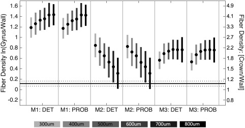
Gyral bias is dependent on MRI resolution. Fiber tracking is performed using three tracking strategies, at image resolutions ranging from 300 μm isotropic to 800 μm isotropic. The log‐ratio of density at the gyral crowns to that at the walls is shown for all algorithms, and all resolutions. Results are shown without subsequent quantification (i.e., no scaling factor)

3.8. Effect of higher order diffusion model

We next ask whether the ability to detect multiple fiber orientations in a voxel enables more anatomically correct streamline propagation into the cortex. CSD has been shown to be both accurate and consistent in resolving multiple intravoxel fiber populations, and has been used extensively to study crossing fibers throughout the brain(Jeurissen, Leemans, Tournier, Jones, & Sijbers, 2013; Tournier et al., 2007, 2008). Figure 10 shows the voxel‐wise reconstruction results for both DTI and CSD in two gyral blades. For DTI (middle column), 3D ellipsoids are shown representing the average diffusion distance in each direction. WM glyphs show the typical “cigar” shape, while more isotropic ellipsoids are apparent along the WMGM boundary along with a lower FA, likely indicating larger geometric fiber dispersion or multiple fiber populations. The CSD glyphs (right column) show the estimated fiber orientation distributions. Many areas in both WM and GM show multiple fiber populations. In addition, in agreement with previous studies (Dyrby et al., 2011; Leuze et al., 2014; Miller et al., 2011), we see fibers largely oriented radially (perpendicular) to the WMGM boundary, particularly in the crowns (solid arrows), and crossing fibers oriented tangentially to the boundary that are especially prevalent in the walls (solid arrows). Also of note, the short U‐shaped fiber tract occurring between the faces of adjacent sulci (white brackets) are apparent in both diffusion techniques. Even here, CSD often shows the presence of second fiber population oriented perpendicular to the surface, although occupying a much smaller volume fraction in each voxel (see Discussion, Section 4.1).

Figure 10.

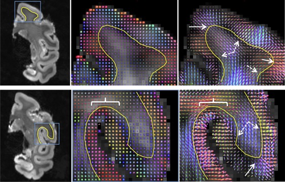
CSD shows evidence of multiple fiber populations along the WMGM boundary. DTI ellipsoids (middle column) and CSD fiber orientation glyphs (right column) are shown for SFG (top row) and PRG (bottom row). WMGM boundary is shown as a yellow line. Fibers are largely perpendicular to the WMGM surface at the crowns (solid arrow), while crossing fibers (not detectable using DTI) are prevalent along the walls and in GM (dashed arrow). Dense U‐fibers just below the cortical surface are visible between adjacent sulci (white brackets) [Color figure can be viewed at http://wileyonlinelibrary.com]

Figure 11 shows the results of CSD (Tournier et al., 2007, 2012, 2008) with both deterministic and probabilistic tractography. Comparing these results with Figure 4, CSD has a modest reduction of gyral bias (∼1%–20% reduction) compared to DTI. In addition, multiple combinations of seeding and scaling strategies are no longer (statistically) significantly biased. However, these results still tend to overestimate the density at the crowns relative to walls. In other words, although the bias is reduced below a statistically detectable level, there is still a numeric difference between the tractography results and the ground truth histology, but we did not have sufficient power to detect a significant difference.

Figure 11.

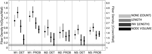
CSD streamline bias is reduced compared to DTI (compare to Figure 4), but is still greater than histological ground truth. Mean (circle) and 95% confidence intervals (vertical line) are shown over all gyri for each CSD tracking algorithm. Four quantification strategies include (1) no scaling, (2) scaling by length, (3) inverse streamline length, and (4) inverse node volume. Histological mean and 95% confidence intervals across all gyri are shown as horizontal solid and dotted lines

Qualitatively, the tractography results show high levels of similarity with those from DTI (Supporting Information, Figure 3); however, the ability of streamlines to propagate in multiple directions is now apparent in both WM and GM. Similarly, the dominant source of bias from these tractography results comes from the longer fibers (Supporting Information, Figure 4), where, in all cases, longer fibers are more biased toward the crowns than medium and short fibers. However, this bias is reduced (for all lengths) when compared to DTI tractography (compare to Figure 6). Angular agreement in CSD orientation estimates was also assessed (Supporting Information, Figure 5). The angular differences along the WMGM boundary were slightly improved compared to DTI, with first, second, and, third quartiles of −8.5°, −0.7°, and 7.3°, respectively, a reduction likely due to the reduced partial volume effects of multiple fiber orientations along the boundary. The median absolute angular difference in WM was 7.9°, again, a slightly better value than for the diffusion tensor.

4. DISCUSSION

Using dMRI tractography to map the neuronal connections of the brain requires accurately estimating connections between large numbers of gray matter regions. In this study, we have shown that there is a significant bias for dMRI tractography streamlines to terminate on gyral crowns, relative to the sulcal banks—an artifact that could significantly affect the results of any quantitative estimates of connectivity using dMRI. It appears that this gyral bias is significant in many gyral blades across the entire brain, and occurs even with exceptionally high‐quality ex vivo data. This effect was shown for a range of tracking algorithms, including both deterministic and probabilistic, and varying model complexities, from the simple diffusion tensor (Figures 3 and 4), to a model capable of describing a complex fiber orientation distribution (Figure 11). Additionally, this gyral bias occurred for a range of diffusion weightings (Supporting Information, Figure 2), and even for exceptionally high‐resolution datasets (Figure 9).

These results have several implications for current tractography practices. As described in (Jones et al., 2013), the use of the “fiber count” and similar terminology is likely an inaccurate metric to describe the true connection strength between two regions derived from diffusion tractography. However, these measures are widely used in the literature (Jones et al., 2013), particularly in mapping connectomes (Hagmann et al., 2010, 2008, 2007; Honey et al., 2009). Here, we have shown that a “count” of the streamlines crossing the WMGM boundary does not accurately represent the fiber count in the same regions derived from histological measurements. In fact, no fiber quantification strategy consistently yielded a connectivity measure that was not biased relative to histology. This does not, however, invalidate existing connectivity studies; rather than true measures of connectivity, these graph‐theoretical measures and streamline connections reflect some characteristics of the underlying white matter microstructure, with some level of uncertainty and bias. This work focuses on one of several potential sources of fiber tracking bias.

The results from this study should also provide guidance for future generations of tracking algorithms. Specifically, we have shown that nearly orthogonal bending over the range of a millimeter, particularly along sulcal walls, is not uncommon. While the average curvature of axons crossing the WMGM border is relatively small (∼20°/voxel, see Figure 7), there is tremendous variation across the brain, as the gyral blades take a variety of different geometries and sizes (see Figure 1). Thus, there is a tradeoff when choosing a curvature threshold parameter. A liberal threshold is necessary to track properly into the cortex, but too high a threshold may result in a loss of tracking specificity (Thomas et al., 2014), and potentially anatomically unrealistic tracks. Even so, very liberal thresholds (including no curvature threshold) still numerically overestimated the connectivity at the gyral crowns. Alternatively, there is a possibility to modify the rules of fiber tracking, possibly at the cortex (Van Essen et al., 2014). Some groundwork has already been laid toward a histology‐informed model of diffusion near the cortex by Cottaar et al. (2016, 2015), but as of yet, no fiber tracking results using modified rules have been reported. However, applying anatomically informed constraints to fiber tracking algorithms terminations and rejection criteria was proposed in (Smith et al., 2012), which shows encouraging results, including a more homogenous density of streamlines along the cortical ribbon (see figure 6 in Smith et al., 2012).

In addition, there is a class of emerging tractography methods in the literature (Daducci, Dal Palu, Lemkaddem, & Thiran, 2015; Qi, Meesters, Nicolay, Ter Haar Romeny, & Ossenblok, 2016; Smith et al., 2013) in which whole‐brain streamline reconstruction is forced to match the diffusion imaging data, ensuring that the streamline density in each voxel is more reflective of the underlying biological fiber density at that location. If the streamlines approaching any surface of the WMGM boundary have an appropriate spatial density distribution, the gyral bias should disappear (Yeh et al., 2016). While these methods have been shown to result in more accurate streamline quantification in simulation, phantom, and in vivo studies, they have not been validated against histologically defined fiber densities. Results from these techniques, and future tracking strategies, can be compared to our histological results to ensure plausible connectivity measures that are anatomically meaningful.

Finally, although this observed bias causes both false positive (overestimation of fiber termination on gyri) and false negative (underestimation on sulci) connectivity measures, it may not present a significant issue in studies of the human connectome. Because many connectome analyses study regional differences in connectivity at the scale of the entire gyral blade, biases in connection patterns and subsequent graph theoretical measures may be mitigated by coarse parcellation schemes. For example, a parcellation scheme based on gyral‐based regions of interest (Desikan et al., 2006), or a relatively low number of regions (∼30–70) (Destrieux et al., 2010; Fischl et al., 2004) will probably be less affected by gyral bias than a scheme with ∼1000 cortical nodes (Hagmann et al., 2008).

4.1. Sources of bias: Seeding, curvature, partial volume effects, and fiber propagation

Overall, it appears that the observation that streamlines are denser in gyral crowns than along the sulcal banks may be influenced by a variety of factors. The dominant source of gyral bias is the over‐representation of longer fibers due to whole brain and white matter seeding. We show that these long and medium length fibers tend to terminate on gyral crowns, and contribute most to the bias (Figure 6). Importantly, scaling the connectivity profile by the inverse fiber length does not eliminate the observed gyral bias. While this empirical normalization does reduce the gyral bias relative to histology, applying this scaling de‐emphasizes almost all neighborhood and long association pathways, as well as all commissural fibers—fibers which form important components of the brains connectome. While seeding from the WMGM boundary partially alleviates this problem (Figure 4), there still exists a bias toward the gyral crown in many gyral blades (Figure 3), with an average 2× higher connectivity at the crowns that walls. It is important to note that because scaling by inverse fiber length is specifically intended to compensate for homogenous white matter seeding, the application of this metric (although it reduces bias) is not appropriate with WMGM seeding. With DTI tractography, no combination of seeding and subsequent scaling matches the profiles obtained with histological analysis.

Our analysis of myelin‐stained sections showed a higher overall curvature of fibers at the sulcal wall compared to the relatively low curvature at the crowns (Figure 7). We hypothesized that a higher curvature threshold would allow more streamlines to enter the cortex, resulting in a reduced gyral bias. However, we found that the curvature threshold did not affect the overall bias (Supporting Information, Figure 1), although it almost certainly does affect anatomical accuracy (which we did not assess). Analysis of individual gyral blades (Figure 7, G and H) shows that myelinated axons can curve by as much as 50 degrees per voxel (over 400 μm in this dataset) as they enter the gray matter. This means that (assuming perfect orientation estimates), the curvature threshold should be set to at least 50 degrees, and likely even higher with lower resolution datasets.

Partial volume effects due to subcortical white matter could cause a bias in orientation estimates along the WMGM boundary to point toward the gyral crown, which would result in a gyral bias in subsequent tractography (Van Essen et al., 2014). Our validation of orientation information on a voxel‐by‐voxel basis shows that there is a slight propensity for the estimated orientations to be biased toward the gyral crown (by a median value of just 2.2°). This is observed in data acquired at 400 μm isotropic resolution, and is likely to be even worse in human datasets at 2+ mm voxel sizes.

Finally, in the case of a local reconstruction algorithm that is able to reconstruct complex fiber geometries, biases could result due to assumptions inherent in the propagation method of choice. For example, high angular resolution diffusion imaging techniques are able to resolve multiple fiber orientations along the WMGM boundary (Figure 10), in agreement with histology (Sotiropoulos et al., 2013a). However, most tracking algorithms will choose to follow the path with least angular deviation, rather than make the sharp turns necessary to exit the white matter (even if the curvature threshold allows for it). This explains, at least partially, why a gyral bias is still observed in Figure 11, where we have chosen to use CSD for local reconstruction. Similar difficulties of fiber tracks reaching certain cortical areas have been previously documented in the macaque brain (Reveley et al., 2015). Using dMRI from high resolution ex vivo specimens, Reveley et al. find that a large portion of the cortical surface is inaccessible to fiber tractography. They attribute these results to dense sheets of white matter axons parallel to the WMGM boundary and just beneath the cortex (for example, the U‐fibers seen in our Figure 10), which inhibit appropriate cortical termination. Even if dMRI is able to detect multiple fiber populations in these superficial white matter bundles (Figure 10), the tracking algorithm is unlikely to follow the correct orientation, which may have not only a larger deviation angle, but a smaller volume fraction component in that voxel. The large areas of the cortex inaccessible to tracking are also visible in our data (see Figure 5, dashed arrow), and lie predominantly in sulci. Here, we find that the gyral bias is not only caused by intervoxel (superficial white matter bundles) and intravoxel (crossing fibers) WM geometries, but is modulated by seeding and stopping strategies, and subsequent track weighting and scaling strategies.

4.2. Resolution

Because the dimensions of the dMRI voxel are orders of magnitude larger than the structures the technique aims to trace (2–3 mm vs 1–20 μm, respectively), image resolution is a clear limitation when it comes to brain connectivity studies (Jones et al., 2013). Thus, it is advantageous to increase the spatial resolution (at the expense of SNR) as much as possible to minimize the partial volume effects of crossing or bending fibers, and, hopefully, better identify white matter insertion points into the cortex. Results from the Human Connectome Project (Sotiropoulos et al., 2013b; Sporns, 2013; Ugurbil et al., 2013), and other studies pushing the current resolution limits of dMRI (Heidemann et al., 2012; Jeong, Gore, & Anderson, 2013), including ex vivo imaging (D'Arceuil et al., 2007; McNab et al., 2009), show promise in more accurately tracking white matter pathways into the cortex.

The results for M2 in our studies seems contradictory (Figure 9), where the gyral bias becomes worse as voxel size decreases. This could have two potential explanations. First, is the over‐representation of large white matter tracks (as previously described), which are now seeded more frequently due to smaller voxel volumes. Second, the larger voxel size may cause the fibers within the cortex to have an increased influence on fiber orientations sampled in the WM. This can be due to both partial volume effects between WM and GM, and due to interpolation of orientation information during the tracking process itself. Because the cortical fiber orientations are largely tangential to the WMGM boundary (Figure 7), the estimated fiber orientations in larger voxels may be rotated toward the cortex, causing streamlines entering gyral blades to exit the WM along the sulcal bank before they reach the crowns. It is interesting that M1 does not show share the same trend, even though it will also be affected by homogenous WM seeding. The only difference between M1 and M2 is the inclusion of the GM as a seed region for M1. This suggests that a large source of the bias comes from seeding in the cortex itself. For example, seeds placed in the sulcal wall or fundi may only propagate a few voxels before encountering orthogonal fibers of the underlying WM and terminate propagation due to excessive curvature. Because this propagation is (at most) the length of the cortex, these fibers often do not meet the minimum length threshold. In contrast, fibers seeded from the crown can easily propagate into the deep WM (Figure 5). Both contrasting effects on gyral bias are, in part, partially alleviated with WMGM boundary seeding (Figure 9).

4.3. Histology

This study is important also from a purely histological perspective. The (non)uniformity of the cortex has implications for evolution, cortical organization, connectional architecture, and cerebral development or morphology. Rather than a structurally uniform cortex (Braitenberg, Schu¨Z, & Braitenberg, 1998; Carlo & Stevens, 2013; Rockel et al., 1980), it has recently been shown that there is variation of neuronal density both across species (Herculano‐Houzel, Collins, Wong, Kaas, & Lent, 2008), and within‐species across major cortical areas (Charvet, Cahalane, & Finlay, 2015; Collins, 2011; Herculano‐Houzel et al., 2008). Here, we show that the density of axons entering (or leaving) the white matter actually varies even within‐gyrus, from gyral crown to sulcal walls. Using a similar parcellation scheme based on convexity, Hilgetag and Barbas (2006) found an increase in neuron number in the deep layers (cortical layers V and VI) of the gyrus compared to the same layers of the sulcal and intermediate (sulcal banks) regions, results that are in agreement with our studies. Because the architectural connections of cortical areas are influenced by their location within the gyral blade, the potential exists for future parcellation schemes to further distinguish cortical areas based on structural connectivity.

4.4. Study limitations

There are a number of potential limitations to this study. The most significant is the method for counting histological fibers crossing the WMGM boundary—if the boundary is too deep into white matter, the estimated density would be too high, and too shallow a boundary would make the fiber count too low. To limit errors in fiber counting, we've made these measurements across the entire gyral blade in each section, as well as across multiple independent sections (>4) per region of interest. Further, it can be seen (Figure 3) that the variability in these histological density measurements is much less than that estimated from dMRI fiber tracking. Another major limitation is the 2D nature of the histological sections. Recent work has extended histological analysis to 3D (Jespersen, Leigland, Cornea, & Kroenke, 2012; Khan et al., 2015; Schilling et al., 2016), however, analysis is limited to small fields‐of‐view, and characterization of multiple whole slices in 3D is a significant technological challenge. In addition, because we are only staining and imaging myelin, our histology is not sensitive to nonmyelinated tissue structures (including unmyelinated axons, dendrites, and glial cells) that may contribute to diffusion anisotropy, particularly in the cortex (Jespersen et al., 2012). In addition, our measurements are simply quantifying the agreement (or lack thereof) between the histological “myelinated axon count” and diffusion tractography “fiber count,” with the common assumption that streamline density should be in some way related to the number or density (or some measure of connectivity) of axons (in our case, myelinated axons).

Finally, our histological “fiber density” is a simple count of the axons entering the cortex. We do not attempt to determine cortico‐cortical connectivity in this study, meaning we have no knowledge of the specific fiber pathway followed other than the fact that the fiber left the white matter and entered the gray matter. The myelinated axons in our study cannot be related or attributed to a specific tract system. A full characterization of gyral‐gyral, gyral‐sulcal, and sulcal‐sulcal connectivity would lend significant support (or opposition) to the various morphogenesis and morphological theories of cortical structure (Hilgetag & Barbas, 2006; Nie et al., 2012). Similarly, it would be of interest to be able to determine where in the gyral blade those fibers entering the cortex came from. For example, do fibers that form the center of the gyral “stalk” tend to enter the crowns, while those near the periphery “peel‐off” from the stalk as they enter the cortex (Van Essen et al., 2014)? Visual inspection of myelin‐stained or neuron‐stained histological slices suggests this is the case in at least some regions. However, a full characterization of this organization would require tracing individual fibers throughout the entire gyral blade, and could enable the development of future tracking algorithms that use anatomical priors to enhance the accuracy of these techniques. We not aware of any studies quantifying the distribution of labeled fibers which could determine whether long‐ or short‐range fibers are expected to terminate preferentially on the crown or walls, nor that determine specific fiber systems that are affected by this bias.

All data, including diffusion MRI, histology, and regions of interest, are made freely available at https://www.nitrc.org/projects/E39Macaque/ for study replication or utilization in future validation studies.

5. CONCLUSION

In this study, using histology as a tool for validation, we have shown that there is a bias of fiber tracking algorithms to terminate on gyral crowns. We first show that many gyral regions in the brain have denser histological fiber connectivity than do neighboring sulcal walls. Next, we find that DTI fiber tracking algorithms are significantly biased toward the gyral crowns in many gyral blades. The source of this gyral bias is most heavily dependent on seeding strategy and subsequent connectivity quantification (i.e., scaling). We also find that myelinated fibers curve more at sulcal walls than they do at crowns. However, the curvature threshold of DTI tracking algorithms does not have a significant effect on the bias. A comparison with histological fiber trajectories shows that the underlying dMRI estimated fiber orientations are also biased toward gyral crowns. We then show that this tractography gyral bias still persists with more advanced diffusion models and tracking algorithms, and over a wide range of MRI acquisition resolutions. It is important to keep these limitations in mind when interpreting dMRI connectivity studies. Tracking algorithms may be able to incorporate this anatomical information when constructing streamline trajectories and determining appropriate seeding and stopping criteria. Future dMRI studies may need to incorporate anatomical priors and constraints, or non‐dMRI information, to accurately determine the structural connectivity of the brain.

Supporting information

Additional Supporting Information may be found online in the supporting information tab for this article.

Supporting Information Figure Legends

Supporting Information Figure S1

Supporting Information Figure S2

Supporting Information

Supporting Information

Supporting Information

Schilling K, Gao Y, Janve V, Stepniewska I, Landman BA, Anderson AW. Confirmation of a gyral bias in diffusion MRI fiber tractography. Hum Brain Mapp. 2018;39:1449–1466. 10.1002/hbm.23936

REFERENCES

- Aitchison, J. (1986). The statistical analysis of compositional data (Vol. XV, p. 416). London, New York: Chapman and Hall. [Google Scholar]
- Alexander, D. C. , & Barker, G. J. (2005). Optimal imaging parameters for fiber‐orientation estimation in diffusion MRI. NeuroImage, 27, 357–367. [DOI] [PubMed] [Google Scholar]
- Alexander, D. C. , Pierpaoli, C. , Basser, P. J. , & Gee, J. C. (2001). Spatial transformations of diffusion tensor magnetic resonance images. IEEE Transactions on Medical Imaging, 20, 1131–1139. [DOI] [PubMed] [Google Scholar]
- Allen, J. S. , Damasio, H. , & Grabowski, T. J. (2002). Normal neuroanatomical variation in the human brain: An MRI‐volumetric study. American Journal of Physical Anthropology, 118, 341–358. [DOI] [PubMed] [Google Scholar]
- Anderson, A. W. (2001). Theoretical analysis of the effects of noise on diffusion tensor imaging. Magnetic Resonance in Medicine, 46, 1174–1188. [DOI] [PubMed] [Google Scholar]
- Bakker, R. , Tiesinga, P. , & Kotter, R. (2015). The Scalable Brain Atlas: Instant web‐based access to public brain atlases and related content. Neuroinformatics, 13, 353–366. [DOI] [PMC free article] [PubMed] [Google Scholar]
- Basser, P. J. , Mattiello, J. , & LeBihan, D. (1994a). Estimation of the effective self‐diffusion tensor from the NMR spin echo. Journal of Magnetic Resonance. Series B, 103, 247–254. [DOI] [PubMed] [Google Scholar]
- Basser, P. J. , Mattiello, J. , & LeBihan, D. (1994b). MR diffusion tensor spectroscopy and imaging. Biophysical Journal, 66, 259–267. [DOI] [PMC free article] [PubMed] [Google Scholar]
- Basser, P. J. , Pajevic, S. , Pierpaoli, C. , Duda, J. , & Aldroubi, A. (2000). In vivo fiber tractography using DT‐MRI data. Magnetic Resonance in Medicine, 44, 625–632. [DOI] [PubMed] [Google Scholar]
- Behrens, T. E. , & Johansen‐Berg, H. (2005). Relating connectional architecture to grey matter function using diffusion imaging. Philosophical Transactions of the Royal Society of London. Series B Biological Sciences, 360, 903–911. [DOI] [PMC free article] [PubMed] [Google Scholar]
- Bigun, J. , & Granlund, G. H. (1987). Optimal orientation detection of linear symmetry. June. p 433–438.
- Braitenberg, V. , Schu¨Z, A. , & Braitenberg, V. (1998). Cortex: Statistics and geometry of neuronal connectivity (Vol. xiii, p. 249). Berlin, New York: Springer. [Google Scholar]
- Budde, M. D. , & Annese, J. (2013). Quantification of anisotropy and fiber orientation in human brain histological sections. Frontiers in Integrative Neuroscience, 7, 3. [DOI] [PMC free article] [PubMed] [Google Scholar]
- Budde, M. D. , & Frank, J. A. (2012). Examining brain microstructure using structure tensor analysis of histological sections. NeuroImage, 63, 1–10. [DOI] [PubMed] [Google Scholar]
- Calamante, F. , Tournier, J. D. , Jackson, G. D. , & Connelly, A. (2010). Track‐density imaging (TDI): Super‐resolution white matter imaging using whole‐brain track‐density mapping. NeuroImage, 53, 1233–1243. [DOI] [PubMed] [Google Scholar]
- Carlo, C. N. , & Stevens, C. F. (2013). Structural uniformity of neocortex, revisited. Proceedings of the National Academy of Sciences, 110, 1488–1493. [DOI] [PMC free article] [PubMed] [Google Scholar]
- Caruyer, E. , Lenglet, C. , Sapiro, G. , & Deriche, R. (2013). Design of multishell sampling schemes with uniform coverage in diffusion MRI. Magnetic Resonance in Medicine, 69, 1534–1540. [DOI] [PMC free article] [PubMed] [Google Scholar]
- Chang, L.‐C. , Koay, C. G. , Pierpaoli, C. , & Basser, P. J. (2007). Variance of estimated DTI‐derived parameters via first‐order perturbation methods. Magnetic Resonance in Medicine, 57, 141–149. [DOI] [PubMed] [Google Scholar]
- Charvet, C. J. , Cahalane, D. J. , & Finlay, B. L. (2015). Systematic, cross‐cortex variation in neuron numbers in rodents and primates. Cerebral Cortex, 25, 147–160. [DOI] [PMC free article] [PubMed] [Google Scholar]
- Chen, H. , Zhang, T. , Guo, L. , Li, K. , Yu, X. , Li, L. , … Liu, T. (2013). Coevolution of gyral folding and structural connection patterns in primate brains. Cerebral Cortex, 23, 1208–1217. [DOI] [PMC free article] [PubMed] [Google Scholar]
- Choe, A. S. , Gao, Y. , Li, X. , Compton, K. B. , Stepniewska, I. , & Anderson, A. W. (2011). Accuracy of image registration between MRI and light microscopy in the ex vivo brain. Magnetic Resonance Imaging, 29, 683–692. [DOI] [PMC free article] [PubMed] [Google Scholar]
- Choe, A. S. , Stepniewska, I. , Colvin, D. C. , Ding, Z. , & Anderson, A. W. (2012). Validation of diffusion tensor MRI in the central nervous system using light microscopy: Quantitative comparison of fiber properties. NMR in Biomedicine, 25, 900–908. [DOI] [PMC free article] [PubMed] [Google Scholar]
- Clayden, J. D. (2013). Imaging connectivity: MRI and the structural networks of the brain. Functional Neurology, 28, 197–203. [PMC free article] [PubMed] [Google Scholar]
- Collins, C. E. (2011). Variability in neuron densities across the cortical sheet in primates. Brain, Behavior and Evolution, 78, 37–50. [DOI] [PubMed] [Google Scholar]
- Cottaar, M. , Bastiani, M. , Chen, C. , Dikranian, K. , Van Essen, D. C. , Behrens, T. E. , … Jbabdi, S. (2016). Fibers crossing the white/gray matter boundary: A semi‐global, histology‐informed dMRI model. Singapore.
- Cottaar, M. , Jbabdi, S. , Glasser, M. F. , Dikranian, K. , Van Essen, D. C. , Behrens, T. E. , & Sotiropoulos, S. N. (2015). A generative model of white matter axonal orientations near the cortex. Toronto, Canada.
- D'Arceuil, H. E. , Westmoreland, S. , & de Crespigny, A. J. (2007). An approach to high resolution diffusion tensor imaging in fixed primate brain. NeuroImage, 35, 553–565. [DOI] [PubMed] [Google Scholar]
- Daducci, A. , Dal Palu, A. , Lemkaddem, A. , & Thiran, J. P. (2015). COMMIT: Convex optimization modeling for microstructure informed tractography. IEEE Transactions on Medical Imaging, 34, 246–257. [DOI] [PubMed] [Google Scholar]
- Dale, A. M. , Fischl, B. , & Sereno, M. I. (1999). Cortical surface‐based analysis. I. Segmentation and surface reconstruction. NeuroImage, 9, 179–194. [DOI] [PubMed] [Google Scholar]
- Desikan, R. S. , Segonne, F. , Fischl, B. , Quinn, B. T. , Dickerson, B. C. , Blacker, D. , … Killiany, R. J. (2006). An automated labeling system for subdividing the human cerebral cortex on MRI scans into gyral based regions of interest. NeuroImage, 31, 968–980. [DOI] [PubMed] [Google Scholar]
- Destrieux, C. , Fischl, B. , Dale, A. , & Halgren, E. (2010). Automatic parcellation of human cortical gyri and sulci using standard anatomical nomenclature. NeuroImage, 53, 1–15. [DOI] [PMC free article] [PubMed] [Google Scholar]
- Donahue, C. J. , Sotiropoulos, S. N. , Jbabdi, S. , Hernandez‐Fernandez, M. , Behrens, T. E. , Dyrby, T. B. , … Glasser, M. F. (2016). Using diffusion tractography to predict cortical connection strength and distance: A quantitative comparison with tracers in the monkey. The Journal of Neuroscience, 36, 6758–6770. [DOI] [PMC free article] [PubMed] [Google Scholar]
- Dyrby, T. B. , Baare, W. F. , Alexander, D. C. , Jelsing, J. , Garde, E. , & Sogaard, L. V. (2011). An ex vivo imaging pipeline for producing high‐quality and high‐resolution diffusion‐weighted imaging datasets. Human Brain Mapping, 32, 544–563. [DOI] [PMC free article] [PubMed] [Google Scholar]
- Dyrby, T. B. , Sogaard, L. V. , Hall, M. G. , Ptito, M. , & Alexander, D. C. (2013). Contrast and stability of the axon diameter index from microstructure imaging with diffusion MRI. Magnetic Resonance in Medicine, 70, 711–721. [DOI] [PMC free article] [PubMed] [Google Scholar]
- Fischl, B. , Sereno, M. I. , & Dale, A. M. (1999). Cortical surface‐based analysis. II: Inflation, flattening, and a surface‐based coordinate system. NeuroImage, 9, 195–207. [DOI] [PubMed] [Google Scholar]
- Fischl, B. , van der Kouwe, A. , Destrieux, C. , Halgren, E. , Segonne, F. , Salat, D. H. , … Dale, A. M. (2004). Automatically parcellating the human cerebral cortex. Cerebral Cortex, 14, 11–22. [DOI] [PubMed] [Google Scholar]
- Gallyas, F. (1971). Silver staining of Alzheimer's neurofibrillary changes by means of physical development. Acta Morphologica Academiae Scientiarum Hungaricae, 19, 1–8. [PubMed] [Google Scholar]
- Girard, G. , Whittingstall, K. , Deriche, R. , & Descoteaux, M. (2014). Towards quantitative connectivity analysis: Reducing tractography biases. NeuroImage, 98, 266–278. [DOI] [PubMed] [Google Scholar]
- Gong, G. , Jiang, T. , Zhu, C. , Zang, Y. , Wang, F. , Xie, S. , … Guo, X. (2005). Asymmetry analysis of cingulum based on scale‐invariant parameterization by diffusion tensor imaging. Human Brain Mapping, 24, 92–98. [DOI] [PMC free article] [PubMed] [Google Scholar]
- Hagmann, P. , Cammoun, L. , Gigandet, X. , Gerhard, S. , Grant, P. E. , Wedeen, V. , … Sporns, O. (2010). MR connectomics: Principles and challenges. Journal of Neuroscience Methods, 194, 34–45. [DOI] [PubMed] [Google Scholar]
- Hagmann, P. , Cammoun, L. , Gigandet, X. , Meuli, R. , Honey, C. J. , Wedeen, V. J. , & Sporns, O. (2008). Mapping the structural core of human cerebral cortex. PLoS Biology, 6, e159. [DOI] [PMC free article] [PubMed] [Google Scholar]
- Hagmann, P. , Kurant, M. , Gigandet, X. , Thiran, P. , Wedeen, V. J. , Meuli, R. , & Thiran, J.‐P. (2007). Mapping human whole‐brain structural networks with diffusion MRI. PLoS One, 2, e597. [DOI] [PMC free article] [PubMed] [Google Scholar]
- Heidemann, R. M. , Anwander, A. , Feiweier, T. , Knosche, T. R. , & Turner, R. (2012). k‐space and q‐space: Combining ultra‐high spatial and angular resolution in diffusion imaging using ZOOPPA at 7 T. NeuroImage, 60, 967–978. [DOI] [PubMed] [Google Scholar]
- Herculano‐Houzel, S. , Collins, C. E. , Wong, P. , Kaas, J. H. , & Lent, R. (2008). The basic nonuniformity of the cerebral cortex. Proceedings of the National Academy of Sciences of the United States of America, 105, 12593–12598. [DOI] [PMC free article] [PubMed] [Google Scholar]
- Hilgetag, C. C. , & Barbas, H. (2006). Role of mechanical factors in the morphology of the primate cerebral cortex. PLoS Computational Biology, 2, e22. [DOI] [PMC free article] [PubMed] [Google Scholar]
- Honey, C. J. , Sporns, O. , Cammoun, L. , Gigandet, X. , Thiran, J. P. , Meuli, R. , & Hagmann, P. (2009). Predicting human resting‐state functional connectivity from structural connectivity. Proceedings of the National Academy of Sciences, 106, 2035–2040. [DOI] [PMC free article] [PubMed] [Google Scholar]
- Jeong, H. K. , Gore, J. C. , & Anderson, A. W. (2013). High‐resolution human diffusion tensor imaging using 2‐D navigated multishot SENSE EPI at 7 T. Magnetic Resonance in Medicine, 69, 793–802. [DOI] [PMC free article] [PubMed] [Google Scholar]
- Jespersen, S. N. , Leigland, L. A. , Cornea, A. , & Kroenke, C. D. (2012). Determination of axonal and dendritic orientation distributions within the developing cerebral cortex by diffusion tensor imaging. IEEE Transactions on Medical Imaging, 31, 16–32. [DOI] [PMC free article] [PubMed] [Google Scholar]
- Jeurissen, B. , Leemans, A. , Tournier, J. D. , Jones, D. K. , & Sijbers, J. (2013). Investigating the prevalence of complex fiber configurations in white matter tissue with diffusion magnetic resonance imaging. Human Brain Mapping, 34, 2747–2766. [DOI] [PMC free article] [PubMed] [Google Scholar]
- Jones, D. K. , & Basser, P. J. (2004). Squashing peanuts and smashing pumpkins”: How noise distorts diffusion‐weighted MR data. Magnetic Resonance in Medicine, 52, 979–993. [DOI] [PubMed] [Google Scholar]
- Jones, D. K. , Knosche, T. R. , & Turner, R. (2013). White matter integrity, fiber count, and other fallacies: The do's and don'ts of diffusion MRI. NeuroImage, 73, 239–254. [DOI] [PubMed] [Google Scholar]
- Khan, A. R. , Cornea, A. , Leigland, L. A. , Kohama, S. G. , Jespersen, S. N. , & Kroenke, C. D. (2015). 3D structure tensor analysis of light microscopy data for validating diffusion MRI. NeuroImage, 111, 192–203. [DOI] [PMC free article] [PubMed] [Google Scholar]
- Kleinnijenhuis, M. , van Mourik, T. , Norris, D. G. , Ruiter, D. J. , van Cappellen van Walsum, A. M. , & Barth, M. (2015). Diffusion tensor characteristics of gyrencephaly using high resolution diffusion MRI in vivo at 7T. NeuroImage, 109, 378–387. [DOI] [PubMed] [Google Scholar]
- Knosche, T. R. , Anwander, A. , Liptrot, M. , & Dyrby, T. B. (2015). Validation of tractography: Comparison with manganese tracing. Human Brain Mapping, 36, 4116–4134. [DOI] [PMC free article] [PubMed] [Google Scholar]
- Lazar, M. , & Alexander, A. L. (2003). An error analysis of white matter tractography methods: Synthetic diffusion tensor field simulations. NeuroImage, 20, 1140–1153. [DOI] [PubMed] [Google Scholar]
- Le Bihan, D. , Breton, E. , Lallemand, D. , Grenier, P. , Cabanis, E. , & Laval‐Jeantet, M. (1986). MR imaging of intravoxel incoherent motions: Application to diffusion and perfusion in neurologic disorders. Radiology, 161, 401–407. [DOI] [PubMed] [Google Scholar]
- Leergaard, T. B. , White, N. S. , de Crespigny, A. , Bolstad, I. , D'arceuil, H. , Bjaalie, J. G. , & Dale, A. M. (2010). Quantitative histological validation of diffusion MRI fiber orientation distributions in the rat brain. PLoS One, 5, e8595. [DOI] [PMC free article] [PubMed] [Google Scholar]
- Leuze, C. W. , Anwander, A. , Bazin, P. L. , Dhital, B. , Stuber, C. , Reimann, K. , … Turner, R. (2014). Layer‐specific intracortical connectivity revealed with diffusion MRI. Cerebral Cortex, 24, 328–339. [DOI] [PMC free article] [PubMed] [Google Scholar]
- Li, C. , Huang, R. , Ding, Z. , Gatenby, C. , Metaxas, D. , & Gore, J. (2008). A variational level set approach to segmentation and bias correction of images with intensity inhomogeneity. Medical Image Computing and Computer‐Assisted Intervention, 11, 1083–1091. [DOI] [PMC free article] [PubMed] [Google Scholar]
- Li, G. , Guo, L. , Nie, J. , & Liu, T. (2009). Automatic cortical sulcal parcellation based on surface principal direction flow field tracking. NeuroImage, 46, 923–937. [DOI] [PMC free article] [PubMed] [Google Scholar]
- Li, K. , Guo, L. , Li, G. , Nie, J. , Faraco, C. , Cui, G. , … Liu, T. (2010). Gyral folding pattern analysis via surface profiling. NeuroImage, 52, 1202–1214. [DOI] [PMC free article] [PubMed] [Google Scholar]
- Liptrot, M. G. , Sidaros, K. , & Dyrby, T. B. (2014). Addressing the path‐length‐dependency confound in white matter tract segmentation. PLoS One, 9, e96247. [DOI] [PMC free article] [PubMed] [Google Scholar]
- Mars, R. B. , Jbabdi, S. , Sallet, J. , O'reilly, J. X. , Croxson, P. L. , Olivier, E. , … Rushworth, M. F. (2011). Diffusion‐weighted imaging tractography‐based parcellation of the human parietal cortex and comparison with human and macaque resting‐state functional connectivity. Journal of Neuroscience, 31, 4087–4100. [DOI] [PMC free article] [PubMed] [Google Scholar]
- McNab, J. A. , Jbabdi, S. , Deoni, S. C. , Douaud, G. , Behrens, T. E. , & Miller, K. L. (2009). High resolution diffusion‐weighted imaging in fixed human brain using diffusion‐weighted steady state free precession. NeuroImage, 46, 775–785. [DOI] [PubMed] [Google Scholar]
- McNab, J. A. , Polimeni, J. R. , Wang, R. , Augustinack, J. C. , Fujimoto, K. , Stevens, A. , … Wald, L. L. (2013). Surface based analysis of diffusion orientation for identifying architectonic domains in the in vivo human cortex. NeuroImage, 69, 87–100. [DOI] [PMC free article] [PubMed] [Google Scholar]
- Miller, K. L. , Stagg, C. J. , Douaud, G. , Jbabdi, S. , Smith, S. M. , Behrens, T. E. , … McNab, J. A. (2011). Diffusion imaging of whole, post‐mortem human brains on a clinical MRI scanner. NeuroImage, 57, 167–181. [DOI] [PMC free article] [PubMed] [Google Scholar]
- Mori, S. , Crain, B. J. , Chacko, V. P. , & van Zijl, P. C. (1999). Three‐dimensional tracking of axonal projections in the brain by magnetic resonance imaging. Annals of Neurology, 45, 265–269. [DOI] [PubMed] [Google Scholar]
- Nie, J. , Guo, L. , Li, K. , Wang, Y. , Chen, G. , Li, L. , … Liu, T. (2012). Axonal fiber terminations concentrate on gyri. Cerebral Cortex, 22, 2831–2839. [DOI] [PMC free article] [PubMed] [Google Scholar]
- Parker, C. S. , Deligianni, F. , Cardoso, M. J. , Daga, P. , Modat, M. , Dayan, M. , … Clayden, J. D. (2014). Consensus between pipelines in structural brain networks. PLoS One, 9, e111262. [DOI] [PMC free article] [PubMed] [Google Scholar]
- Paxinos, G. , Huang, X. F. , & Toga, A. W. (2000). The rhesus monkey brain in stereotaxic coordinates (p. 163). San Diego, CA: Academic Press. [Google Scholar]
- Peters, A. , & Jones, E. G. (1984). Cerebral cortex. New York: Plenum Press. [Google Scholar]
- Qi, S. , Meesters, S. , Nicolay, K. , Ter Haar Romeny, B. M. , & Ossenblok, P. (2016). Structural brain network: What is the effect of LiFE optimization of whole brain tractography? Frontiers in Computational Neuroscience, 10, 12. [DOI] [PMC free article] [PubMed] [Google Scholar]
- Reveley, C. , Seth, A. K. , Pierpaoli, C. , Silva, A. C. , Yu, D. , Saunders, R. C. , … Ye, F. Q. (2015). Superficial white matter fiber systems impede detection of long‐range cortical connections in diffusion MR tractography. Proceedings of the National Academy of Sciences, 112, E2820–E2828. [DOI] [PMC free article] [PubMed] [Google Scholar]
- Rockel, A. J. , Hiorns, R. W. , & Powell, T. P. (1980). The basic uniformity in structure of the neocortex. Brain, 103, 221–244. [DOI] [PubMed] [Google Scholar]
- Rohde, G. K. , Aldroubi, A. , & Dawant, B. M. (2003). The adaptive bases algorithm for intensity‐based nonrigid image registration. IEEE Transactions on Medical Imaging, 22, 1470–1479. [DOI] [PubMed] [Google Scholar]
- Ronen, I. , Budde, M. , Ercan, E. , Annese, J. , Techawiboonwong, A. , & Webb, A. (2014). Microstructural organization of axons in the human corpus callosum quantified by diffusion‐weighted magnetic resonance spectroscopy of N‐acetylaspartate and post‐mortem histology. Brain Structure and Function, 219, 1773–1785. [DOI] [PubMed] [Google Scholar]
- Schilling, K. , Janve, V. , Gao, Y. , Stepniewska, I. , Landman, B. A. , & Anderson, A. W. (2016). Comparison of 3D orientation distribution functions measured with confocal microscopy and diffusion MRI. NeuroImage, 129, 185–197. [DOI] [PMC free article] [PubMed] [Google Scholar]
- Schmahmann, J. D. , & Pandya, D. (2009). Fiber pathways of the brain. USA: OUP. [Google Scholar]
- Schmahmann, J. D. , & Pandya, D. N. (2007). Cerebral white matter–historical evolution of facts and notions concerning the organization of the fiber pathways of the brain. Journal of the History of the Neuroscience, 16, 237–267. [DOI] [PubMed] [Google Scholar]
- Smith, R. E. , Tournier, J. D. , Calamante, F. , & Connelly, A. (2012). Anatomically‐constrained tractography: Improved diffusion MRI streamlines tractography through effective use of anatomical information. NeuroImage, 62, 1924–1938. [DOI] [PubMed] [Google Scholar]
- Smith, R. E. , Tournier, J. D. , Calamante, F. , & Connelly, A. (2013). SIFT: Spherical‐deconvolution informed filtering of tractograms. NeuroImage, 67, 298–312. [DOI] [PubMed] [Google Scholar]
- Sotiropoulos, S. N. , Chen, C. , Dikranian, K. , Jbabdi, S. , Behrens, T. E. , Van Essen, D. C. , & Glasser, M. F. (2013a). Comparison of diffusion MRI predictions and histology in the Macaque brain. Salt Lake City, Utah. p 835.
- Sotiropoulos, S. N. , Jbabdi, S. , Xu, J. , Andersson, J. L. , Moeller, S. , Auerbach, E. J. , … Consortium, W. U.‐M. H. (2013b). Advances in diffusion MRI acquisition and processing in the Human Connectome Project. NeuroImage, 80, 125–143. [DOI] [PMC free article] [PubMed] [Google Scholar]
- Sporns, O. (2013). The human connectome: Origins and challenges. NeuroImage, 80, 53–61. [DOI] [PubMed] [Google Scholar]
- Sporns, O. , Tononi, G. , & Kotter, R. (2005). The human connectome: A structural description of the human brain. PLoS Computational Biology, 1, e42. [DOI] [PMC free article] [PubMed] [Google Scholar]
- Thomas, C. , Ye, F. Q. , Irfanoglu, M. O. , Modi, P. , Saleem, K. S. , Leopold, D. A. , & Pierpaoli, C. (2014). Anatomical accuracy of brain connections derived from diffusion MRI tractography is inherently limited. Proceedings of the National Academy of Sciences, 111, 16574–16579. [DOI] [PMC free article] [PubMed] [Google Scholar]
- Tournier, J. D. , Calamante, F. , & Connelly, A. (2007). Robust determination of the fibre orientation distribution in diffusion MRI: Non‐negativity constrained super‐resolved spherical deconvolution. NeuroImage, 35, 1459–1472. [DOI] [PubMed] [Google Scholar]
- Tournier, J. D. , Calamante, F. , & Connelly, A. (2012). MRtrix: Diffusion tractography in crossing fiber regions. International Journal of Imaging Systems and Technology, 22, 53–66. [Google Scholar]
- Tournier, J. D. , Calamante, F. , & Connelly, A. (2013). Determination of the appropriate b value and number of gradient directions for high‐angular‐resolution diffusion‐weighted imaging. NMR in Biomedicine, 26, 1775–1786. [DOI] [PubMed] [Google Scholar]
- Tournier, J. D. , Yeh, C. H. , Calamante, F. , Cho, K. H. , Connelly, A. , & Lin, C. P. (2008). Resolving crossing fibres using constrained spherical deconvolution: Validation using diffusion‐weighted imaging phantom data. NeuroImage, 42, 617–625. [DOI] [PubMed] [Google Scholar]
- Ugurbil, K. , Xu, J. , Auerbach, E. J. , Moeller, S. , Vu, A. T. , Duarte‐Carvajalino, J. M. , … Consortium, W. U.‐M. H. (2013). Pushing spatial and temporal resolution for functional and diffusion MRI in the Human Connectome Project. NeuroImage, 80, 80–104. [DOI] [PMC free article] [PubMed] [Google Scholar]
- Van Essen, D. C. , & Maunsell, J. H. (1980). Two‐dimensional maps of the cerebral cortex. The Journal of Comparative Neurology, 191, 255–281. [DOI] [PubMed] [Google Scholar]
- Van Essen, D. C. J. , S., Sotiropoulos , N., Chen , C., Dikranian , E., Coalson , T., Harwell , J., Behrens , T., & Glasser, M. (2014). Mapping connections in humans and non‐human primates: Aspirations and challenges for diffusion imaging In Johansen‐Berg H., Behrens T.E.J. (Eds.), Diffusion MRI: From quantitative measurement to in‐vivo neuroanatomy (2nd ed, pp. 337–358). London, UK; Waltham, MA: Elsevier/Academic Press. [Google Scholar]
- Yeatman, J. D. , Dougherty, R. F. , Myall, N. J. , Wandell, B. A. , & Feldman, H. M. (2012). Tract profiles of white matter properties: Automating fiber‐tract quantification. PLoS One, 7, e49790. [DOI] [PMC free article] [PubMed] [Google Scholar]
- Yeh, C. H. , Smith, R. E. , Liang, X. , Calamante, F. , & Connelly, A. (2016). Correction for diffusion MRI fibre tracking biases: The consequences for structural connectomic metrics. NeuroImage. [DOI] [PubMed] [Google Scholar]
Associated Data
This section collects any data citations, data availability statements, or supplementary materials included in this article.
Supplementary Materials