Optimized Inversion-Time schedules for quantitative T₁ measurements based on high-resolution Multi-Inversion EPI

Abstract

PURPOSE

Demonstrate an optimized multi-inversion EPI technique to accelerate quantitative T₁ mapping by judicious selection of inversion times for each slice.

METHODS

Slice ordering is optimized to maximize discrimination between tissues with different T₁ values. The optimized slice orderings are tested in the ISMRM/NIST phantom and compared to an unoptimized 21-measurement acquisition. The utility of the method is demonstrated in a healthy subject in vivo at 3T and validated with a gold-standard inversion-recovery sequence. The in vivo precision of our technique was tested by repeated scans of the same subject within a scan session and across scan sessions occurring 28 days apart.

RESULTS

Phantom measurements yielded good agreement (R² = 0.99) between the T₁ estimates from the proposed optimized protocol, reference values from the NIST phantom and gold-standard inversion-recovery values, as well as a negligible estimation bias that was slightly lower than that from the unoptimized 21-measurement protocol (0.74 ms vs. 19 ms). The range of values for the scan-rescan coefficient of variation was 0.86–0.93 (within-session) and 0.83–0.92 (across-sessions) across all scan durations tested.

CONCLUSION

Optimized slice orderings allow faster quantitative T₁ mapping. The optimized sequence yielded accurate and precise T₁ maps.

Introduction

Two-dimensional inversion recovery (IR) pulse sequences are commonly used for quantitative T₁ mapping. To estimate T₁, each image slice is acquired with multiple inversion time (TI) values and the measured image intensities are then fitted to a model to extract the underlying quantitative T₁ recovery value at each voxel. Although reliable, this T₁ mapping procedure suffers from lengthy acquisition durations that prevent its use in routine clinical scans. To increase efficiency, rather than acquiring only one slice per IR faster alternatives acquire multiple slices sequentially following each non-spatially-selective inversion pulse such that each of the slices is acquired at different TI [1–3]. The temporal ordering of the slices is permuted from one IR period to the next, such that during the repeated inversion recoveries each slice is measured with a distinct ordering of TI values. This multiple-slice scheme provides increased signal in each measured slice relative to the Look-Locker approach [4–6] in which the same slice is excited and acquired multiple times during the IR to sample multiple TI values with the disadvantage that there is little time for signal recovery (longitudinal relaxation) in the slice between excitations. In the multiple-slice scheme, the repetition time (TR) for any given slice may vary from one IR period to the next, and in general for fast acquisitions TR is too short for complete longitudinal recovery (in some cases TR < T₁), therefore fitting the T₁ value using a closed-form model can be challenging [7,8]. Instead, the resulting image intensities for a given slice can be matched to a dictionary of signal recovery curves pre-computed using the Bloch simulation of the specific pulse sequence for a variety of possible T₁ values [9].

The image acquisition during the IR can be accomplished with different image encoding schemes but the echo-planar-imaging (EPI) sequence offers compelling benefits. In addition to a rapid acquisition, EPI is the most commonly used acquisition technique for functional MRI (fMRI) [10], as well as diffusion and perfusion MRI [11], which are typically acquired alongside separate anatomical reference scans to localize regions of interest. Because EPI is vulnerable to geometric distortion due to its low phase encoding bandwidth [12], the EPI data must be distortion corrected to achieve an accurate geometric alignment to anatomical reference images obtained with standard pulse sequences such as magnetization-prepared rapid gradient echo (MPRAGE), for example [13,14]. The limited accuracy of distortion correction has driven recent interest in EPI based anatomical reference data using the same phase encoding bandwidth used in the functional (or diffusion/perfusion) acquisition to perfectly match the geometric distortion of the two datasets [15–20].

In previous work [9] we described a multi-inversion EPI sequence to provide a quantitative T₁ map that is distortion-matched to EPI-based fMRI data. To ensure accurate reconstruction of the multiple different T₁ values present in the human brain, multiple measurements were acquired across multiple IR periods and the slice order permuted by a constant ‘skip-factor’ between each measurement, with the skip-factor defined as the offset from a linear ordering of N slices, i.e. the number of slices permuted or “skipped” at the beginning of the IR period and acquired at the end. Unfortunately, given the broad range of T₁ values in the human brain, a large number of measurements are needed to acquire the required broad range of TI values in each slice for accurate T₁ mapping, resulting in prolonged scan time for a single volume (up to 3 minutes). Moreover, the choice of skip-factor is arbitrary and not optimized for the anatomy of interest.

Instead, in this work we use concepts originally developed for flip angle and TR schedule optimization in MR Fingerprinting [21–25] to select the optimal slice ordering, namely one that produces the set of distinct TI values sampled by each slice that maximizes the discrimination between different tissue types for a presumed range of tissue T₁ values. We demonstrate that this optimization allows reducing the required number of measurements without adversely affecting the quantitative accuracy and precision of the T₁ maps obtained. Our method is demonstrated in phantom data and in an in vivo dataset from a healthy subject scanned at 3T.

Theory

Reconstruction dictionary design

We briefly review here the design of the reconstruction dictionary. The reader is referred to Ref. [9] for further details. Let TI_j,k be the inversion time undergone by a slice j in measurement k in a given slice ordering scheme. Since the acquisition time of each slice is constant, the inversion times can be converted into a specific slice order by dividing by the acquisition time per slice. The evolution of the signal intensity S in each voxel within a given slice j can be modeled as a vector d(T₁)=[S(TI_j,1), S(TI_j,2), …] where the dependence of the signal on the tissue’s underlying T₁ value is generated by the varying inversion times experienced by that slice. Given a set of TI_j,k values, the signal intensity evolution for tissues with different T₁ values can be calculated using Bloch equation simulations assuming mono-exponential relaxation, zero transverse magnetization and ideal flip angles. After normalization of each vector, the calculated set of signal intensity vectors for the chosen range of T₁ values can be assembled into a matrix D, with one column per T₁ value, which forms the reconstruction dictionary. By finding the best matching dictionary entry to the voxel-wise data acquired from the scanner using a pattern-matching algorithm, such as the vector dot product, the corresponding T₁ value can be identified and assigned to the voxel.

Slice Ordering Optimization

Let N be the number of slices and K be the number of measurements. Optimizing the constant skip-factor slice ordering x= [TI_1,1, TI_2,1,, … TI_N,K] can be accomplished using concepts originally developed for MR Fingerprinting (MRF) schedule optimization [22–25]. In MRF schedule optimization, an optimization dictionary is defined by selecting a range of T₁ values covering the anatomical range of interest representing different tissue types. The magnetization of each tissue is calculated using a Bloch simulation of the acquisition pulse sequence and stored as a column vector which, after normalization of each vector, can be assembled into a matrix H. The similarity between each vector in H and all others can be computed using the vector dot product. The diagonal elements of the dot product matrix H^TH therefore measure the similarity between the signal from a tissue and itself whereas the off-diagonal elements record the similarity with all other tissues, and a low dot product within these off-diagonal elements indicates high discriminability. The schedule of acquisition parameters can then be varied to find the ones that maximize the discriminability between tissues.

In this work, rather than varying the schedule of acquisition parameters, the slice ordering is varied instead. Varying the slice order in a given measurement is equivalent to varying the TI values sampled by each slice, such that each slice samples the signal at a subset of TI times out of the set of available TIs given by (TR/N)·(1, 2, …, N). Since the slice ordering affects all slices simultaneously the optimization dictionary must be expanded into a 3D matrix H_r where r ranges from 1 to N to account for the effect on all slices. The goal of the optimization, however, remains the same—maximizing the discriminability or, equivalently, minimizing the similarity between tissues. The problem can thus be recast as a search for the slice ordering that yields the lowest cost, defined here as the smallest sum of off-diagonal entries in each dot product matrix (H^TH)_r. To avoid focusing the optimization on certain slices at the expense of others, the optimization problem is formulated as a search for the slice ordering that minimizes the maximum cost across all slices:

$$\underset{\mathit{x}}{min}\underset{\mathit{r}}{max}\sum _{i\ne j}{({({\mathit{H}}^T\mathit{H})}_r)}_{ij}(\mathit{x})$$ (1)

This is equivalent to optimizing the discriminability of the ‘worst’ (maximum cost) slice, although it should be noted that the current ‘worst’ slice will change from iteration to iteration during the optimization as the search-space is explored.

Solving the optimization problem

Search-Space Reordering

Equation (1) represents an optimization over a set of permutations. Optimizing over permutations (i.e. the space of all possible orderings of a contiguous set of integers) is a challenging problem, and traditional optimization algorithms are not designed for optimizing over permutation space and are therefore ineffective. Genetic algorithms [26] may be used but require significant computational resources and processing time to converge to a solution. Instead, we apply a mapping to transform the unordered permutation search-space into an ordered vector space [27]. This mapping is performed by assigning an order to permutations; for example, an ordering can be defined for permutations of the ordered set of n integers a = {a₁, a₂, …, a_n} through mapping to a new ordered set of integers b = {b₁, b₂, …, b_n} defined such that b_i equals the number of elements of the set a preceding the location of a_j = i that are greater than i [28]. As an example (taken from [28]), if {a₁, a₂, …, a₈} = {5, 6, 1, 3, 2, 4, 8, 7} then {b₁, b₂, …, b₈} = {2, 3, 2, 2, 0, 0, 1, 0}. This mapping enables the use of faster algorithms that operate on vector spaces [29].

Dynamic Hill Climbing

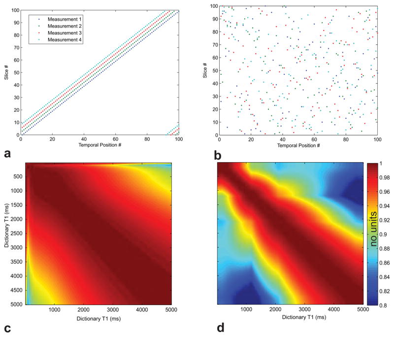
Equation (1) can be solved using the Dynamic Hill Climbing (DHC) algorithm [28]. The algorithm consists of searching the hyperspace for the point (slice ordering) that has the lowest cost as defined by Equation (1). The algorithm is initialized with a slice ordering defined with a constant skip-factor between measurements (Fig. 1a) used in previous work [9]. This ensures that any slice ordering found will improve upon the constant skip-factor slice ordering. The algorithm explores the search-space by defining a random probing vector which is added to the initial point. If the new point improves on the current cost, the probing vector length is increased, otherwise it is decreased. This process is repeated until the probing vector length is below a certain threshold at which point the algorithm moves to the next iteration. The point with the lowest cost found corresponds to the optimal slice ordering (Fig. 1b) with the greatest discriminability (Figs. 1c, d).

Fig. 1.

Example orderings and corresponding dot-product matrices H^TH. (a) The slice ordering for 100 slices corresponding to an optimized acquisition with skip-factor=3. The temporal order of the slice acquisition matches the anatomical order, but with each IR period the starting slice index is incremented by 3 such that in the first IR period the acquisition starts with slice 0, in the second IR period the acquisition starts with slice 3, and so on. (b) The slice orderings for 100 slices corresponding to an optimized acquisition in which the ordering is computed to maximize discriminability of the signal evolution across distinct tissues. (c) The dot-product matrix H^TH for a representative slice corresponding to the unoptimized case. The high values off the diagonal indicate poor discriminability. (d) The dot product matrix H^TH for the same slice corresponding to the optimized case shown in panel (b). Lower values off the diagonals of ~5% on average indicate improved discriminability.

Methods

Optimization Cost

Optimized orderings for protocols consisting of 100 slices were generated by defining an optimization-dictionary with T₁ values in the range 100–5000 ms in intervals of 50 ms. Slice orderings were generated with 4, 5, 8, 10 and 16 measurements and their optimization costs (i.e. their discrimination) were compared. An additional, 21-measurement ordering with a constant skip-factor 3 was used for comparison with our previously published protocol [9]. Similar length slice orderings were generated for 25 and 50 slices and their optimization costs compared as well. The optimization algorithm was allowed to run for 50,000 iterations to ensure adequate coverage of the search-space which required approximately 8–40 hours, depending on the slice ordering length and the number of measurements, on a 2.4 GHz Core i7 Dell laptop with 16 GB RAM and 256 GB hard drive.

MRI

Phantom Experiments

For phantom experiments, a 3T Tim Trio (Siemens Healthcare, Erlangen, Germany) whole-body scanner was used with the manufacturer’s body coil for transmit and 12-channel head array coil for receive. The TR/TI/TE/BW was set to 6690 ms/13 ms/27 ms/2170 Hz/pixel. The resolution was set to 1.2×1.2×1.2 mm³ with a matrix of 192×192. An acceleration factor of R=4 was used along with FLEET autocalibration [30,31] prior to acquisition and the images were reconstructed online using the GRAPPA [32] method. A non-spatially selective adiabatic inversion pulse [33] ensured adequate inversion of the spins in the presence of spatial nonuniformity of transmit efficiency (due to dielectric effects).

In Vivo Human Experiments

For human experiments, the same TR/TI/TE/R/BW and resolution were used as in the Phantom Experiments section above but with a 32-channel head array for reception. Total scan time for the 4/5/8/10/16 and 21 measurements was 33/40/60/74/114 and 147 s, respectively. For the same spatial coverage, a 1×1×1 mm³ isotropic acquisition would require an additional 6–8 seconds for each scan. Although fat suppression is commonly used in EPI experiments to avoid chemical shift artifacts, in this work fat suppression was disabled in all in vivo experiments to avoid biasing the T₁ quantification (see below for explanation of the fat suppression bias).

Estimation of T₁ values

All data were estimated by calculating the voxel-wise dot-product between the acquired data and the entries of the pre-computed dictionary of signal magnetizations and selecting the best match. The dictionary comprised of T₁ values in the range of 1–5000 ms in intervals of 1 ms.

Phantom

The accuracy and precision of the optimized slice orderings was assessed using the International Society for Magnetic Resonance in Medicine (ISMRM)/National Institute of Standards and Technology (NIST) multi-compartment phantom with calibrated T₁ and T₂ values similar to those of the human brain [34]. The phantom was scanned with the 8-measurement slice ordering and the resulting T₁ maps compared to both the true phantom values (characterized by NIST and calculated using the gold-standard NMR spectroscopy IR sequence) and the un-optimized 21-measurement protocol. Two phantom compartments with the shortest T₁ values (< 30 ms) were excluded from the measurements since their T₁ were comparable with the TE of the EPI sequence.

To rule out any scanner-specific biases, we also validated the true phantom values using the recommended inversion recovery method based on a non-selective IR spin-echo (IR-SE) EPI acquisition. The TR was set to 18 s and TE set to 21 ms. The minimum TI available for this sequence was 21 ms. A logarithmically spaced sampling of 36 TI values was used to ensure accurate fitting of the short T₁ compartments. Total scan time for the 36 inversion times was ~65 minutes. The magnitude-valued images were fitted to the 3-point inversion-recovery signal equation [8] using the Levenberg-Marquadt algorithm ( lsqcurvefit function) in Matlab (Mathworks, Natick, MA).

Fat Suppression

Since fat suppression pulses may affect the T₁ quantification through e.g. magnetization transfer [9,35], the acquisition was repeated both with and without fat suppression pulses for the 8-measurement length. The frequency profile of the fat suppression pulse used on the scanner was computed using a custom-made Bloch equation simulator written in Matlab to determine its potential impact on the water signal (through inadvertent excitation of the water peak).

Slice-specific optimization cost

Because the optimization algorithm uses a single global metric to converge to an optimal slice ordering, once the algorithm converges different slices can have different optimization costs. The resulting slice-specific cost of the optimized 8-measurement protocol was therefore compared to that of the unoptimized 21-measurement protocol.

In Vivo Human

A healthy 29-year-old male subject was recruited for this study and provided informed consent prior to the experiment in accordance with our institution’s Human Research Committee.

Validation

The T₁ map obtained with our method was validated in vivo in a single slice using the same recommended IR-SE EPI sequence and protocol described in the Phantom section above. Total scan time for this one slice sampled at 36 inversion times was ~65 minutes. Three regions corresponding to grey matter, white matter and cerebrospinal fluid (CSF) were selected from each image and the agreement between the mean T₁ values of each region assessed.

Reproducibility

A mask was created to remove all signals extraneous to the head by summing the signal from the 21-measurement protocol and thresholding the resulting volume. The masked T₁ maps from the initial and subsequent scans were co-registered in Matlab ( imregister function) and used to calculate the correlation coefficient for different measurement lengths as a measure of the reproducibility/precision of the estimated in vivo T₁ values. The correlation coefficient was calculated including the CSF from the whole brain. However, we also calculated the correlation coefficient with the CSF removed by thresholding the T₁ maps to remove all voxels with T₁ > 2000 ms.

Following co-registration, spatial variations in the reproducibility were measured for the 8 measurement acquisition by calculating the slice-specific correlation coefficient.

Results

Optimization cost

The (H^TH)_r matrix from a representative slice for a 100-slice unoptimized 21-measurement protocol is shown in Fig. 1c in comparison to an optimized 8-measurement protocol (Fig. 1d). The off-diagonal elements in the optimized matrix are approximately ~5% smaller on average than those of the unoptimized matrix, which indicates improved discriminability in the optimized case.

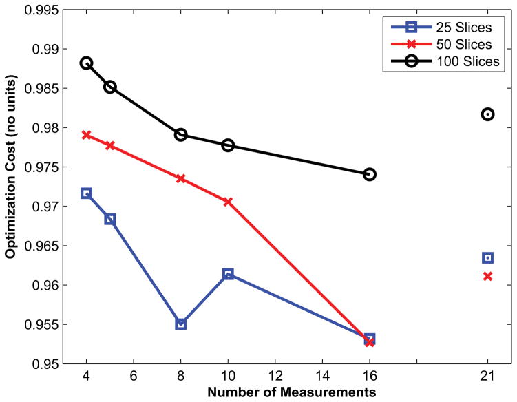
The relationship between the cost of the optimization function and the number of measurements (acquisition length) is shown in Fig. 2 for example orderings with 25, 50 and 100 slices. The optimization cost for slice orderings with fewer slices was correspondingly smaller, as expected, given the smaller slice-ordering search-space. Importantly, for a given number of slices, the cost of the unoptimized 21-measurement protocol was higher than that of the optimized protocols with a smaller number of measurements.

Fig. 2.

Cost of the optimization objective function for increasing number of measurements (acquisition duration) for example slice orderings with 100 (black circles), 50 (red crosses) and 25 (blue triangles) slices. Note that a smaller number of slices resulted in lower cost (i.e. superior discrimination) due to the smaller search-space.

Phantom

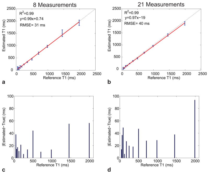
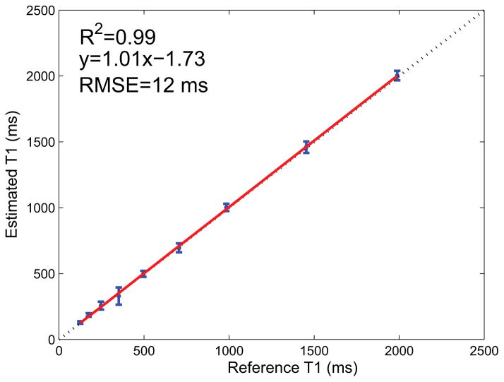
The accuracy of the proposed approach was assessed by estimating T₁ values in the calibrated ISMRM/NIST phantom. The measured and true T₁ values for the optimized 8-measurement and unoptimized 21-measurement acquisition are shown in Fig. 3. The measured T₁ values were derived from the average T₁ value estimated from within each compartment. Compartments with T₁ values similar to the TE of the EPI (T₁ < 30 ms) showed significant error in both protocols, as expected, and were not included in the calculations of the comparison metrics. Such short T₁ values may not be estimable with the current EPI read-out. The Pearson correlation coefficient R was calculated for each acquisition, resulting in an R² value for both acquisition methods tested of 0.99. However, the linear fit shows a small offset of 0.74 ms for the 8-measurement protocol, and for the 21-measurement protocol an offset of 19 ms was calculated indicating a negligible estimation bias associated with this protocol. Unlike the identical R² values, the root mean-squared-error (RMSE) for the 8-measurement protocol was 31 ms which was lower than the 40 ms calculated for the 21-measurement protocol. The estimation absolute error, defined as |Estimated – True|, as a function of the reference T₁ values for each protocol was also calculated and is shown in in Figs. 3c, d. The mean error across all compartments (excluding the short T₁ compartments) was found to be 25 ms for the optimized 8-measurement acquisition and 33 ms for the unoptimized 21-measurment acquisition. Despite the ~3-fold reduction in scan time, the 8-measurement protocol showed excellent agreement with the true phantom values. The measured and true T₁ values for the IR-SE EPI sequence are shown in Fig. 4. In contrast to the 8-measurement protocol, which correctly reconstructed compartments with T₁ values as short as 30 ms, the IR-SE EPI sequence showed significant errors for compartments with T₁ values shorter than 100 ms which were therefore not included in the R² or RMSE calculations. However, the remaining compartments showed excellent agreement to the true phantom values (R²=0.99), a negligible estimation bias (an offset of 1.7 ms) and an RMSE of 12 ms demonstrating that any scanner-specific biases are minimal.

Fig. 3.

T₁ estimation accuracy evaluated in the calibrated ISMRM/NIST phantom. Shown is a comparison between the true and measured compartment T₁ values for an optimized 8-measurement protocol (a) and an unoptimized 21-measurement protocol (b). The dashed line in each plot is the identity line whereas the red line is the least-squares fit line. The error bars represent the standard deviation of the measured T₁ values within the compartment. Note the larger bias in the 21-measurement protocol. The estimation error as a function of the reference phantom T₁ values are shown in (c) for the 8-measurement protocol and in (d) for the 21-measurement protocol.

Fig. 4.

Comparison of the ISMRM/NIST calculated phantom T₁ values to those of a non-selective IR-SE EPI sequence. The true and measured compartment T₁ values are shown along with the identity line (dashed line) and the least-squares fit line (red line). Note that compartments with T₁s smaller than 100 ms showed significant error and were not included in the comparison.

Fat Suppression

The presence of the fat suppression pulse increased the error in the measured T₁ values (see Figs. 5a, b), particularly for long T₁ compartments. Specifically, the RMSE for the 8-measurement protocol was 76 ms for acquisitions with fat suppressions but 31 ms for those without fat suppression. Although the fat suppression pulse is centered on the frequency corresponding to the lipid chemical shift, the simulated frequency profile (Fig. 5c) showed that ~2% of the water signal is also excited (and subsequently dephased) for each slice-selective excitation.

Fig. 5.

True and measured compartment T₁ values calculated from calibrated ISMRM/NIST phantom data for the optimized 8-measurement protocol without (a) and with (b) the presence of a fat suppression pulse. The dashed line is the identity line whereas the red line is the least-squares fit line. The fat saturation pulse (c) centered on the lipids chemical shift nevertheless excites ~2% of the water signal for every slice-selective excitation pulse. The deviation from the identity line is larger in the fat suppression case.

Slice-specific optimization cost

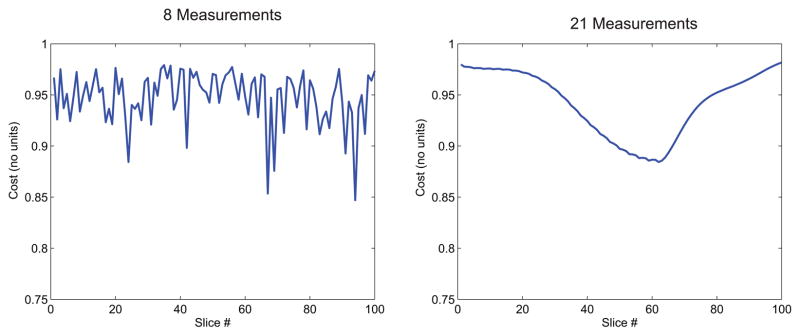
The optimization cost of each slice for an 8-measurement acquisition is shown in Fig. 6a and that of the 21-measurement protocol in Fig. 6b. Because each slice is assigned a distinct acquisition schedule and thus a distinct collection of TI values, each slice in the acquisition has a somewhat different cost in the final schedule generated from the optimization. The slice optimization cost can thus provide a metric for a priori confidence in, or for predicting the expected accuracy of, the T₁ estimates and a guide to judge whether the optimization process, which may terminate within a local minimum, should be allowed to continue in order to further reduce estimation error. (See below in Discussion for a consideration of the potential uses for this ability to predict estimation error.)

Fig. 6.

Optimization cost of each slice for an 8-measurement acquisition (a) and an unoptimized 21-measurement acquisition (b). Higher cost indicates lower discrimination between different T₁ values that may lead to increased error in the reconstructed T₁ maps.

Since each slice also samples a distinct set of TI values, for each 100-slice protocol we calculated the range of TI values (defined as the maximum TI minus the minimum TI) for each slice, then summarized the effect of the number of measurements on the range of TI values by the mean and standard deviation of the range across all slices. The results of this calculation are presented in Supporting Table 1. For the optimized slice orderings, as expected the mean TI value range increases with increasing number of measurements, while the standard deviation decreases. The mean range of TI values was similar for the optimized 8-measurement protocol and the unoptimized 21-measurement protocol, but the standard deviation of the range of TI values was lower in nearly all of the optimized protocols compared to the unoptimized 21-measurement protocol, indicating that the ranges of TI values sampled in the optimized protocols were more consistent across slices.

In Vivo Human Brain

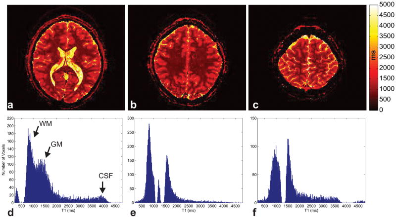
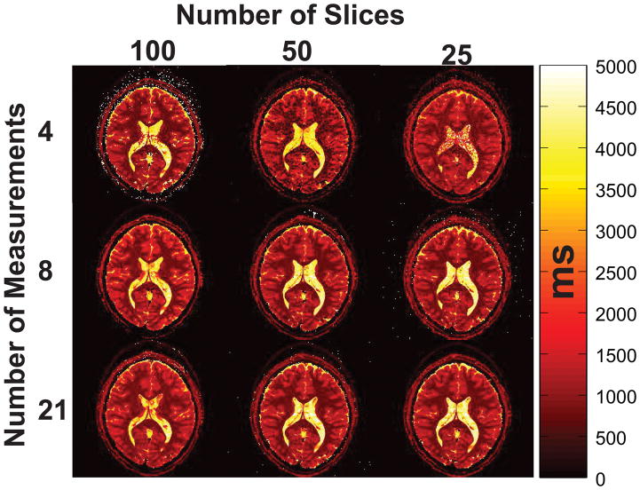
Reconstructed T₁ maps for the 8-measurement protocol of the 100-slice case are shown in Fig. 7 for three different example slices along with a histogram of each slice’s calculated T₁ values. The various peaks visible the histograms (Figs. 7d–f) correspond to literature values of T₁ at 3T [36] of the white matter (~900 ms), gray matter (~1600 ms) and CSF (~4000 ms) tissues further validating the proposed method. Gaps in the histograms of the different slices are in part a result of anatomical features (e.g. scalp, CSF) that are less prevalent in some slices leading to low voxel counts for the corresponding T₁ values, as well as slice-dependent fitting inaccuracies described in the Calculating Expected T₁ Mapping Accuracy from the Dictionary Discrimination section below. A comparison of the same slice for the 100, 50 and 25 slices case for 4, 8 and 21 measurements is shown in Fig. 8 (remaining measurements are shown in Supporting Figure 1). The T₁ maps of the entire volume for all measurement lengths tested are shown in Supporting Figures S2–S7. The proton density (PD) weighted S₀ maps obtained with the optimized 8 measurement in comparison to those of the unoptimized 21 measurement protocol are shown in Supporting Figure S8 and demonstrate the close similarity between the two maps estimated using the optimized and unoptimized protocols.

Fig. 7.

Example quantitative T₁ maps within the brain for three sample slices (a–c) out of the optimized 8-measurement 100-slice acquisition. The color scale indicates the T₁ value in units of ms. The histogram of T₁ values for each slice shown in (d–f) shows distinct peaks corresponding to the white matter, gray matter, and CSF.

Fig. 8.

Reconstructed T₁ maps for a representative slice for 4,8 and 21 measurements for the 100, 50 and 25 slices case.

Validation

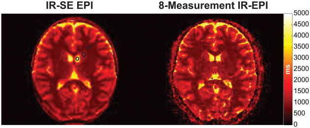
The T₁ map from a single slice estimated by the recommended IR-SE sequence is shown in Fig. 9 in comparison to that obtained with the proposed method. The mean±std grey matter/white matter/CSF T₁ values from the recommended IR-SE sequence were 767±16.0/1130±47.0/4120±264 ms and showed good agreement to the 767±74.0/1160±96.0/3830± 299 ms estimated with the proposed 8-measurement protocol. We also attempted to register the single-slice T₁ map from the recommended IR-SE sequence to the same-session T₁-EPI data, and within this slice found an R² value of 0.64 across all voxels. The R² value for the same comparison based on the NIST/ISMRM phantom was 0.99 over a similar range of T₁ values, suggesting some loss of agreement due to participant motion and misalignment.

Fig. 9.

In vivo T₁ map from a single slice estimated with the recommended IR-SE sequence in comparison to the T₁ map obtained with the 8-measurement optimized protocol for the same slice. The black circles indicate the locations of the grey matter, white matter and CSF regions used to compare the agreement between the two methods.

Reproducibility

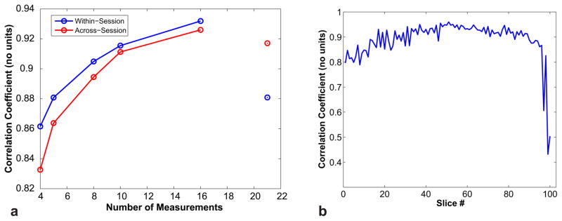
The variation in the correlation coefficient as a function of the number of measurements is shown in Fig. 10a for the across- and within-session acquisitions. The CSF was included in this calculation since its removal had a negligible effect on the correlation coefficient. The within-session correlation coefficient is, on average, ~2% higher than the across-session coefficient, likely due to the smaller shift in head position between within-session scans compared to across-session scans—because there is a slice-specific T₁ estimation error, differential head motion between scans will reduce the precision of the estimate. Both coefficients show an increase in the correlation coefficient with increasing number of measurements, reaching a value of ~0.90 for the within-session 8-measurement protocol used in this study. The within-session correlation coefficient for the 21-measurement protocol was an outlier at ~0.88, which is slightly lower than expected given the ~0.91 across-session coefficient; this is likely due to the abrupt subject motion observed before this run.

Fig. 10.

The scan-rescan correlation coefficient as a function of the number of measurements for the across- and within-session acquisitions (a). The optimized acquisitions show good repeatability despite a significantly shorter scan length. The within-session, slice-specific correlation coefficients for the 8 measurements protocols are shown in (b) to illustrate the spatial variation of the correlation coefficient.

The spatial variation in the within-session slice-specific correlation coefficient for the 8 measurements acquisition is shown in Fig. 10b. As expected, slices outside the brain containing little tissue yielded the minimum correlation of ~0.43. In contrast, slices in the center of the brain showed the greatest reproducibility with a correlation coefficient of ~0.96.

Discussion

We have demonstrated that optimization of the slice ordering can maximize discrimination between different tissues to allow accurate reconstruction of the quantitative T₁ maps despite reduced scan time. The accelerated 8-measurement protocol EPI acquisition allows distortion-matched whole-brain quantitative T₁ mapping in approximately 60 s. Several factors may, however, affect the quality of the derived maps, as described below.

Reconstruction Dictionary

Since the signal in each voxel is matched to the pre-computed dictionary, factors that affect the generated dictionary entries may introduce bias into the reconstructed T₁ maps. In particular, the dictionary construction assumed an ideal 180° inversion pulse and zero transverse magnetization which may not hold in reality due to spatial variations in the B₁⁺ transmit field. These concerns are mitigated, however, by the use of adiabatic inversion pulses that are largely immune to B₁⁺ inhomogeneity. Note that errors in the excitation flip angle do not affect the recovery rate hence do not influence the T₁ value estimation and are therefore accounted for by the dictionary normalization. The slice-selective excitation pulses used in our multiple-slice acquisition may introduce biases as well due to off-resonance effects on neighboring slices, such as incidental magnetization transfer [8,37]. However the variable slice ordering (Fig. 1b) may impart additional robustness to this form of bias as well since the time between excitation of a given slice and the measurement of its neighboring slices, which determines the amount of inadvertent magnetization transfer from the slice-selective excitation pulses, will be different from one inversion recovery period to the next and may therefore average out provided a sufficient number measurements. The minimal bias seen in the reconstructed T₁ maps for the optimized protocol (less than 1 ms), as shown in Fig. 3, validates the assumptions made in the dictionary construction but it is nevertheless possible that other sources of bias remain.

Optimization Algorithm

A set of N slices allows a factorial of N (i.e., N!) possible permutations of the ordering. The immensity of the search-space for N > 10 precluded a brute-force search for the globally optimal slice ordering and required the use of optimization algorithms. However, this problem can be formulated as a variation of the Travelling Salesman Problem [38], a problem that has been intensively studied for which multiple heuristics and algorithms exist [39–41]. In this study we used a hill climbing algorithm to search for a local optimum because of its simplicity and speed. However, more sophisticated algorithms are likely to provide a more globally optimal solution and are the subject of ongoing research.

In general, fewer slices will entail a smaller search-space making it more likely for the optimization algorithm to find an ordering with lower cost, as shown in Fig. 2. This suggests that incorporating slice-acceleration techniques such as Simultaneous Multi-Slice (SMS) EPI [42–44], as has been previously proposed for IR-EPI [17,18], which effectively reduces the number of slices, may provide lower cost and therefore higher accuracy assuming the acquisition has a sufficient signal-to-noise ratio (SNR). Of note, the acquisition of multiple slices incurs no SNR penalty for SMS EPI acquisitions other than g-factor reconstruction noise [45]. However, it is important to recall that the size of the search-space is defined by the product of the effective number of slices and the number of measurements, both of which constitute degrees of freedom for the protocol optimization. Since the algorithm is based on a local search it is possible for it to converge to a local minimum, which may be more likely if either the effective number of slices or the number of measurements is large. Put simply, for a given number of slices, finding the optimal ordering for acquisitions with larger number of measurements will be more difficult. For Simultaneous Multi-Slice acquisitions, while the image reconstruction can generate a larger number of slices than conventional EPI methods, the effective number of slices is not increased, and therefore, e.g., a 126-slice acquisition with conventional EPI is expected to typically have higher cost and increased estimation error than an equivalent 126-slice acquisition collected with Simultaneous Multi-Slice techniques. This extension of our approach to Simultaneous Multi-Slice acquisitions will be explored in future work.

Calculating Expected T₁ Mapping Accuracy from the Dictionary Discrimination

In its current implementation, the optimization routine searches for a slice ordering that minimizes a single objective: the maximum cost across all slices. The slice ordering thus obtained, while optimal in a global sense, may yield a solution with a variable cost for every individual slice. Indeed, plotting the cost for each slice in an optimized 8-measurement acquisition shows significant variation between the discrimination of each individual slice (Fig. 6a). A similar, albeit smoother, variation exists in the slice-specific cost of the 21-measurement acquisition (Fig. 6b) with a constant skip-factor scheme. Consequently, the dictionary matching reconstruction in certain slices will be more robust to errors than in other slices. This is evident in the histograms shown in Fig. 7d–f where the estimation error leads to gaps in the voxel count of certain T₁ values. Nevertheless, as demonstrated by the phantom experiments (Fig. 5), this error is small and zero-mean across slices and, importantly, can be predicted from each slice’s optimization cost (Fig. 6). Additionally, it should be noted that slice orderings with a high cost can still yield accurate T₁ maps provided the SNR is sufficiently high to allow distinguishing similar signal evolutions. Nevertheless, for a given SNR level, the optimization cost can be used as an a priori measure of the expected quality of the estimated T₁ map for the given slice, and the optimization can be further iterated as needed to minimize the cost for the particular slice. Alternatively, multi-objective optimization techniques can be used [46,47] to find a slice ordering that minimizes the cost for all slices simultaneously.

Effect of Fat Saturation

The imperfect frequency profile of the fat saturation pulse used resulted in undesired excitation and dephasing of ~2% of the total water signal for every slice-selective excitation given the non-spatially selective nature of the pulse. This effect explains the results shown in Fig. 5, where the cumulative effect of the fat suppression pulse is particularly pronounced for phantom compartments with long T₁ given their long recovery time. This effect could be modeled and incorporated into the Bloch simulation during the dictionary generation in order to account for this effect in the phantom data, however inadvertent magnetization transfer from tissue macromolecules could still contribute to biasing T₁ values in vivo, as previously discussed [48]. Because these magnetization transfer effects are presumably constant over time and accumulate linearly during each IR period, it is possible to model these effects as well [9], however to simplify the modeling in this work we opted to forgo the fat saturation pulse, resulting in small amounts of chemical shift artifact in the data.

Potential Future Applications

Quantitative T₁ mapping is important in numerous applications. Dynamic contrast enhanced (DCE) MRI is commonly used for with pharmacokinetic models to calculate permeability parameters of tumors and other lesions [49]. Because of the lengthy acquisition times, T₁-weighted images are used in practice rather than the quantitative T₁ maps. Since T₁-weighted images are susceptible to confounding factors and bias, this can have a deleterious effect on the accuracy of the perfusion maps obtained. Fast quantitative T₁ mapping provided by the proposed method would remove this source of error and yield more accurate tissue permeability maps.

Conclusion

We have demonstrated a method for optimizing the inversion times used in multi-inversion EPI. The optimized inversion times provide similar precision and accuracy in less time, allowing a ~3-fold reduction in the scan time needed to obtain the quantitative tissue maps as shown in phantom and in a healthy human subject scanned at 3T.

Supplementary Material

Supp info

Supporting Fig. S1. Reconstructed T₁ maps for a representative slice for all measurements for the 100, 50 and 25 slices case.

Supporting Fig. S2. Reconstructed T₁ maps of 100 slices acquired with the optimized 4-measurement protocol.

Supporting Fig. S3. Reconstructed T₁ maps of 100 slices acquired with the optimized 5-measurement protocol.

Supporting Fig. S4. Reconstructed T₁ maps of 100 slices acquired with the optimized 8-measurement protocol.

Supporting Fig. S5. Reconstructed T₁ maps of 100 slices acquired with the optimized 10-measurement protocol.

Supporting Fig. S6. Reconstructed T₁ maps of 100 slices acquired with the optimized 16-measurement protocol.

Supporting Fig. S7. Reconstructed T₁ maps of 100 slices acquired with the unoptimized 21-measurement protocol.

Supporting Fig. S8. S₀ maps for the 8 measurements and 21 measurement protocols. Note the similarity between the maps obtained with the two measurements.

Supporting Table 1: Summary of the TI values sampled as a function of the number of measurements for the 100-slice protocol. The range (max – min) of TI values was computed for each individual slice, the values reported here represent the mean and standard deviation of the range across all slices for each protocol.

References

- 1.Clare S, Jezzard P. Rapid T1 mapping using multislice echo planar imaging. Magn Reson Med. 2001;45:630–634. doi: 10.1002/mrm.1085. [DOI] [PubMed] [Google Scholar]
- 2.de Smit F, Hoogduin H. Fast whole brain T1 mapping at 3 Tesla. RöFo-Fortschritte Auf Dem Geb. Röntgenstrahlen Bildgeb. Verfahr. 2005;177:A1. [Google Scholar]
- 3.Ordidge R, Gibbs P, Chapman B, Stehling M, Mansfield P. High-speed multislice T1 mapping using inversion-recovery echo-planar imaging. Magn Reson Med. 1990;16:238–245. doi: 10.1002/mrm.1910160205. [DOI] [PubMed] [Google Scholar]
- 4.Look DC, Locker DR. Time saving in measurement of NMR and EPR relaxation times. Rev Sci Instrum. 1970;41:250–251. [Google Scholar]
- 5.Gowland P, Mansfield P. Accurate measurement of T1in vivo in less than 3 seconds using echo-planar imaging. Magn Reson Med. 1993;30:351–354. doi: 10.1002/mrm.1910300312. [DOI] [PubMed] [Google Scholar]
- 6.Henderson E, McKinnon G, Lee T-Y, Rutt BK. A fast 3D Look-Locker method for volumetric T 1 mapping. Magn Reson Imaging. 1999;17:1163–1171. doi: 10.1016/s0730-725x(99)00025-9. [DOI] [PubMed] [Google Scholar]
- 7.Stikov N, Boudreau M, Levesque IR, Tardif CL, Barral JK, Pike GB. On the accuracy of T1 mapping: searching for common ground. Magn Reson Med. 2015;73:514–522. doi: 10.1002/mrm.25135. [DOI] [PubMed] [Google Scholar]
- 8.Barral JK, Gudmundson E, Stikov N, Etezadi-Amoli M, Stoica P, Nishimura DG. A robust methodology for in vivo T1 mapping. Magn Reson Med. 2010;64:1057–1067. doi: 10.1002/mrm.22497. [DOI] [PMC free article] [PubMed] [Google Scholar]
- 9.Renvall V, Witzel T, Wald LL, Polimeni JR. Automatic cortical surface reconstruction of high-resolution T 1 echo planar imaging data. NeuroImage. 2016;134:338–354. doi: 10.1016/j.neuroimage.2016.04.004. [DOI] [PMC free article] [PubMed] [Google Scholar]
- 10.Kwong KK, Belliveau JW, Chesler DA, Goldberg IE, Weisskoff RM, Poncelet BP, et al. Dynamic magnetic resonance imaging of human brain activity during primary sensory stimulation. Proc Natl Acad Sci. 1992;89:5675–5679. doi: 10.1073/pnas.89.12.5675. [DOI] [PMC free article] [PubMed] [Google Scholar]
- 11.Kwong KK, Chesler DA, Weisskoff RM, Donahue KM, Davis TL, Ostergaard L, et al. MR perfusion studies with T1-weighted echo planar imaging. Magn Reson Med. 1995;34:878–887. doi: 10.1002/mrm.1910340613. [DOI] [PubMed] [Google Scholar]
- 12.Jezzard P, Balaban RS. Correction for geometric distortion in echo planar images from B0 field variations. Magn Reson Med. 1995;34:65–73. doi: 10.1002/mrm.1910340111. [DOI] [PubMed] [Google Scholar]
- 13.Mugler JP, Brookeman JR. Three-dimensional magnetization-prepared rapid gradient-echo imaging (3D MP RAGE) Magn Reson Med. 1990;15:152–157. doi: 10.1002/mrm.1910150117. [DOI] [PubMed] [Google Scholar]
- 14.Marques JP, Kober T, Krueger G, van der Zwaag W, Van de Moortele P-F, Gruetter R. MP2RAGE, a self bias-field corrected sequence for improved segmentation and T 1-mapping at high field. Neuroimage. 2010;49:1271–1281. doi: 10.1016/j.neuroimage.2009.10.002. [DOI] [PubMed] [Google Scholar]
- 15.van der Zwaag W, Buur P, Versluis M, Marques JP. Distortion-matched T1-maps and bias-corrected T1w-images as anatomical reference for submillimeter-resolution fMRI. Proc. Int. Soc. Magn. Reson. Med; Singapore. 2016. [Google Scholar]
- 16.Huber L, Marrett S, Handwerker DA, Thomas A, Gutierrez B, Ivanov D, et al. Fast Dynamic Measurement of Functional T1 and Grey Matter Thickness Changes During Brain Activation at 7T. Proc. Int. Soc. Magn. Reson. Med; Singapore. 2016. [Google Scholar]
- 17.Grinstead JW, Wang D, Bhat H, Deshpande V, Cauley SF, Setsompop K, et al. Slice-Accelerated Inversion Recovery T1 Mapping. Proc. Int. Soc. Magn. Reson. Med; Milan, Italy. 2014. [Google Scholar]
- 18.Dougherty R, Mezer A, Zhu K, Kerr A, Middione A. Fast Quantitative T1 Mapping With Simultaneous Multi-Slice EPI. Hamburg: 2014. [Google Scholar]
- 19.Renvall V, Witzel T, Wald LL, Polimeni JR. Fast variable inversion-recovery time EPI for anatomical reference and quantitative T1 mapping. Proc. Int. Soc. Magn. Reson. Med; Milan, Italy. 2014. [Google Scholar]
- 20.Kashyap S, Ivanov D, Havlicek M, Poser BA, Uludag K. High-resolution T1-mapping using inversion-recovery EPI and application to cortical depth-dependent fMRI at 7 Tesla. Proc. Int. Soc. Magn. Reson. Med; Singapore. 2016. [Google Scholar]
- 21.Ma D, Gulani V, Seiberlich N, Liu K, Sunshine JL, Duerk JL, et al. Magnetic resonance fingerprinting. Nature. 2013;495:187–92. doi: 10.1038/nature11971. [DOI] [PMC free article] [PubMed] [Google Scholar]
- 22.Cohen O, Sarracanie M, Armstrong BD, Ackerman JL, Rosen MS. Magnetic resonance fingerprinting trajectory optimization. Proc. Int. Soc. Magn. Reson. Med; Milan, Italy. 2014; p. 0027. [Google Scholar]
- 23.Cohen O, Armstrong BD, Sarracanie M, Farrar Christian T, Ackerman Jerome L, Rosen Matthew S. 15T Ultrahigh Field Fast MR Fingerprinting with Optimized Trajectories. Proc. Int. Soc. Magn. Reson. Med; Milan, Italy. 2014; p. 4285. [Google Scholar]
- 24.Cohen O, Sarracanie M, Rosen MS, Ackerman JL. In Vivo Optimized MR Fingerprinting in the Human Brain. Proc. Int. Soc. Magn. Reson. Med; Singapore. 2016; p. 0430. [Google Scholar]
- 25.Cohen O, Rosen MS. Algorithm comparison for schedule optimization in MR fingerprinting. Magn Reson Imaging. 2017 doi: 10.1016/j.mri.2017.02.010. [DOI] [PMC free article] [PubMed] [Google Scholar]
- 26.Davis L. Handbook of genetic algorithms. 1991. [Google Scholar]
- 27.Knuth DE. The art of computer programming: sorting and searching. Vol. 3. Pearson Education; 1998. [Google Scholar]
- 28.Turrini S. Optimization in Permutation Spaces. Western Research Laboratory; 1996. [Google Scholar]
- 29.Yuret D, De La Maza M. Dynamic hill climbing: Overcoming the limitations of optimization techniques. Second Turk. Symp. Artif. Intell. Neural Netw; Citeseer. 1993; pp. 208–212. [Google Scholar]
- 30.Chapman B, Turner R, Ordidge RJ, Doyle M, Cawley M, Coxon R, et al. Real-time movie imaging from a single cardiac cycle by NMR. Magn Reson Med. 1987;5:246–254. doi: 10.1002/mrm.1910050305. [DOI] [PubMed] [Google Scholar]
- 31.Polimeni JR, Bhat H, Witzel T, Benner T, Feiweier T, Inati SJ, et al. Reducing sensitivity losses due to respiration and motion in accelerated echo planar imaging by reordering the autocalibration data acquisition. Magn Reson Med. 2016;75:665–679. doi: 10.1002/mrm.25628. [DOI] [PMC free article] [PubMed] [Google Scholar]
- 32.Griswold MA, Jakob PM, Heidemann RM, Nittka M, Jellus V, Wang J, et al. Generalized autocalibrating partially parallel acquisitions (GRAPPA) Magn Reson Med. 2002;47:1202–1210. doi: 10.1002/mrm.10171. [DOI] [PubMed] [Google Scholar]
- 33.Ordidge RJ, Wylezinska M, Hugg JW, Butterworth E, Franconi F. Frequency offset corrected inversion (FOCI) pulses for use in localized spectroscopy. Magn Reson Med. 1996;36:562–566. doi: 10.1002/mrm.1910360410. [DOI] [PubMed] [Google Scholar]
- 34.Keenan KE, Stupic KF, Boss MA, Russek SE, Chenevert TL, Prasad PV, et al. Multi-site multi-vendor comparison of T1 measurement using ISMRM/NIST system phantom. Proc. Int. Soc. Magn. Reson. Med; Singapore. 2016; p. #3290. [Google Scholar]
- 35.Shin W, Gu H, Yang Y. Incidental magnetization transfer contrast by fat saturation preparation pulses in multislice look-locker echo planar imaging. Magn Reson Med. 2009;62:520–526. doi: 10.1002/mrm.22034. [DOI] [PMC free article] [PubMed] [Google Scholar]
- 36.Bojorquez JZ, Bricq S, Acquitter C, Brunotte F, Walker PM, Lalande A. What are normal relaxation times of tissues at 3 T? Magn Reson Imaging. 2017;35:69–80. doi: 10.1016/j.mri.2016.08.021. [DOI] [PubMed] [Google Scholar]
- 37.Dixon WT, Engels H, Castillo M, Sardashti M. Incidental magnetization transfer contrast in standard multislice imaging. Magn Reson Imaging. 1990;8:417–422. doi: 10.1016/0730-725x(90)90050-c. [DOI] [PubMed] [Google Scholar]
- 38.Hoffman KL, Padberg M, Rinaldi G. Encycl Oper Res Manag Sci. Springer; 2013. Traveling salesman problem; pp. 1573–1578. [Google Scholar]
- 39.Dorigo M, Gambardella LM. Ant colony system: a cooperative learning approach to the traveling salesman problem. IEEE Trans Evol Comput. 1997;1:53–66. [Google Scholar]
- 40.Černý V. Thermodynamical approach to the traveling salesman problem: An efficient simulation algorithm. J Optim Theory Appl. 1985;45:41–51. [Google Scholar]
- 41.Lin S, Kernighan BW. An effective heuristic algorithm for the traveling-salesman problem. Oper Res. 1973;21:498–516. [Google Scholar]
- 42.Setsompop K, Gagoski BA, Polimeni JR, Witzel T, Wedeen VJ, Wald LL. Blipped-controlled aliasing in parallel imaging for simultaneous multislice echo planar imaging with reduced g-factor penalty. Magn Reson Med. 2012;67:1210–1224. doi: 10.1002/mrm.23097. [DOI] [PMC free article] [PubMed] [Google Scholar]
- 43.Feinberg DA, Setsompop K. Ultra-fast MRI of the human brain with simultaneous multi-slice imaging. J Magn Reson. 2013;229:90–100. doi: 10.1016/j.jmr.2013.02.002. [DOI] [PMC free article] [PubMed] [Google Scholar]
- 44.Moeller S, Yacoub E, Olman CA, Auerbach E, Strupp J, Harel N, et al. Multiband multislice GE-EPI at 7 tesla, with 16-fold acceleration using partial parallel imaging with application to high spatial and temporal whole-brain fMRI. Magn Reson Med. 2010;63:1144–1153. doi: 10.1002/mrm.22361. [DOI] [PMC free article] [PubMed] [Google Scholar]
- 45.Barth M, Breuer F, Koopmans PJ, Norris DG, Poser BA. Simultaneous multislice (SMS) imaging techniques. Magn Reson Med. 2016;75:63–81. doi: 10.1002/mrm.25897. [DOI] [PMC free article] [PubMed] [Google Scholar]
- 46.Deb K, Pratap A, Agarwal S, Meyarivan T. A fast and elitist multiobjective genetic algorithm: NSGA-II. Evol Comput IEEE Trans On. 2002;6:182–197. [Google Scholar]
- 47.Knowles JD, Watson RA, Corne DW. Evol Multi-Criterion Optim. Springer; 2001. Reducing local optima in single-objective problems by multi-objectivization; pp. 269–283. [Google Scholar]
- 48.Santyr GE. Magnetization transfer effects in multislice MR imaging. Magn Reson Imaging. 1993;11:521–532. doi: 10.1016/0730-725x(93)90471-o. [DOI] [PubMed] [Google Scholar]
- 49.Shin K, Ahn K, Choi H, Jung S, Kim B, Jeon S, et al. DCE and DSC MR perfusion imaging in the differentiation of recurrent tumour from treatment-related changes in patients with glioma. Clin Radiol. 2014;69:e264–e272. doi: 10.1016/j.crad.2014.01.016. [DOI] [PubMed] [Google Scholar]
Associated Data
This section collects any data citations, data availability statements, or supplementary materials included in this article.
Supplementary Materials
Supporting Fig. S1. Reconstructed T1 maps for a representative slice for all measurements for the 100, 50 and 25 slices case.
Supporting Fig. S2. Reconstructed T1 maps of 100 slices acquired with the optimized 4-measurement protocol.
Supporting Fig. S3. Reconstructed T1 maps of 100 slices acquired with the optimized 5-measurement protocol.
Supporting Fig. S4. Reconstructed T1 maps of 100 slices acquired with the optimized 8-measurement protocol.
Supporting Fig. S5. Reconstructed T1 maps of 100 slices acquired with the optimized 10-measurement protocol.
Supporting Fig. S6. Reconstructed T1 maps of 100 slices acquired with the optimized 16-measurement protocol.
Supporting Fig. S7. Reconstructed T1 maps of 100 slices acquired with the unoptimized 21-measurement protocol.
Supporting Fig. S8. S0 maps for the 8 measurements and 21 measurement protocols. Note the similarity between the maps obtained with the two measurements.