Assessment of contact predictions in CASP12: Co‐evolution and deep learning coming of age

Abstract

Following up on the encouraging results of residue‐residue contact prediction in the CASP11 experiment, we present the analysis of predictions submitted for CASP12. The submissions include predictions of 34 groups for 38 domains classified as free modeling targets which are not accessible to homology‐based modeling due to a lack of structural templates. CASP11 saw a rise of coevolution‐based methods outperforming other approaches. The improvement of these methods coupled to machine learning and sequence database growth are most likely the main driver for a significant improvement in average precision from 27% in CASP11 to 47% in CASP12. In more than half of the targets, especially those with many homologous sequences accessible, precisions above 90% were achieved with the best predictors reaching a precision of 100% in some cases. We furthermore tested the impact of using these contacts as restraints in ab initio modeling of 14 single‐domain free modeling targets using Rosetta. Adding contacts to the Rosetta calculations resulted in improvements of up to 26% in GDT_TS within the top five structures.

Abbreviations

ES

Entropy score

FM

free modeling

GDT_TS

global distance test—total score

L

sequence length

MCC

the Matthews correlation coefficient

MSA

multiple sequence alignment

PR_AUC

area under the precision‐recall curve

TBM

template‐based modeling.

1. INTRODUCTION

The assessment of contact prediction has been a consistent part of the CASP experiment since CASP2 in 1996.1, 2, 3, 4, 5, 6, 7, 8, 9, 10 It has been early noted that long‐range inter‐residue contact information can be a valuable source of information to constrain the conformational space in de novo structure prediction.11, 12, 13 In consequence, a contact‐assisted structure prediction category was introduced in CASP10.14 However different perspectives on the required number and quality of contacts exist. While some focus on the usage of a small number of accurately predicted contacts,13, 15 others consider larger sets even with lower accuracy to be more useful.11, 16 Despite the idea of using evolutionary information to predict contacts solely based on the protein sequence being around for >20 years,17, 18 methods implementing this approach failed to significantly improve the poor performance of contact prediction algorithms up to CASP10 in 2012.9 The realization that previous attempts were flawed by not filtering the true coevolution signals from other indirect effects19 was picked up by multiple groups that integrated this information in their contact prediction methods.20, 21, 22, 23, 24, 25, 26, 27, 28, 29, 30, 31, 32, 33, 34 While an improvement was not immediately apparent in CASP10, the first indication that the new approach was indeed a turning point manifested in CASP11 when MetaPSICOV outperformed the other groups.10 The improvement from an average precision of 22% to 27% for the most challenging target group in CASP11 was already acknowledged as remarkable. In CASP12, we now see a whole new level of prediction performance with an average precision of 47% on a very similar set of targets.

In this article, we present the analysis of the predictions, compare it to the previous CASP experiments and discuss the results of structure prediction with the provided predictions on a limited set of targets.

2. MATERIALS AND METHODS

Participants were requested to predict inter‐residue contacts with an associated probability P_ij. Following the CASP rules, a contact between residues i and j is defined if the Euclidian distance between their C_β carbons (C_α in case of Glycine) is below 8.0 Å. Probabilities should be between 1 and 0. Furthermore, for binary classification, probabilities above 0.5 indicate that residues are predicted to be in contact.

Contacts were classified based on the sequence separation of residues i and j into: Medium‐range (12≤|i – j|≤23) and long‐range (|i – j|≥24) contacts. Only those two sets were considered for evaluation since these are the most relevant for defining the tertiary structure of a protein.

While contact predictions were submitted for all domains including those classified as template‐based modeling (TBM—37 domains), TBM with templates challenging to detect (TBM/FM—19 domains), and free modeling (FM—38 domains), we only focus our analysis on the FM class since this class represents the most relevant use case, namely contact‐assisted structure prediction in cases where no homologous templates are available.

Depending on the specific application, users can have different requirements on the performance of a contact prediction algorithm. For example, some might be more interested in a small number of accurate long‐range contacts, while others strive for larger lists of medium‐range and long‐range contacts tolerating a higher number of false positives within the prediction. We analyzed the performance of predictors on reduced lists using the provided probabilities only for ranking the contacts. These lists included the top10, L/5, and L/2 (L being the sequence length of the target domain) contacts predicted with the highest probability. The prediction performance was assessed using:

$$Precision=\frac{TP}{TP+FP}\cdot 100\%$$

$$Recall=\frac{TP}{TP+FN}\cdot 100\%$$

$$F_1=2\cdot \frac{precision\cdot recall}{precision+recall}\cdot 100\%$$

where TP indicate true positives, FP false positives, and FN false negatives. Due to the fact that those measures are highly correlated in the reduced lists, we focus mainly the analysis on precision as it is the most intuitive measure and the perfect prediction is 100% for all evaluated targets and list sizes. For the full list, precision is however not an adequate measure as it does not provide any information about the fraction of true contacts that has been predicted. Thus, a more appropriate measure is the F1 score, the harmonic mean of precision and recall, which takes the precision of the predicted contacts and the fraction of the true contact set that was predicted into account. Another measure suitable for evaluation of the full sets is the Matthews correlation coefficient (MCC), which provides a balanced measure evaluating the diverse prediction sets using the binary classification based on the 0.5 cut‐off as described previously.9

$$MCC=\frac{TP\cdot TN-FP\cdot F\mathrm{N}}{\sqrt{\left(TP+FP\right)\left(TP+FN\right)\left(TN+FP\right)\left(TN+FN\right)}}$$

One shortcoming of the above‐mentioned measures is that they use the provided probabilities for ranking and as binary classifier but disregard the additional information the probabilities might have. For this purpose, the area under the precision recall curve (AUC_PR) was introduced in CASP10 and is included in the full list assessment as well. For CASP12 we furthermore analyzed how well the reported probability corresponds to a real probability by binning the predicted probabilities and calculating the fraction of true positives for each interval. In a well‐balanced predictor, this fraction should correspond to the probability that is, when considering all contacts predicted with a probability of 0.3, the fraction of True Positives in this list should be 30%.

2.1. Probability weighted measures

Next to the AUC_PR we also calculated variants of the canonical measures that included the predicted probabilities. While these measures include the information content of the probabilities their usage might encourage predictors to optimize probabilities based on them, and in consequence move away from a meaningful distribution. We have thus refrained from using them in this report although they were discussed at the CASP evaluation meeting. These measures are available and explained at the CASP website (predictioncenter.org).

2.2. Alignment depth

With the increasing importance of coevolution data in contact prediction we determined the length‐normalized alignment depth for each domain. For this, the number of diverse effective sequences was retrieved using PSIBLAST (N_{eff_PSIBLAST}) and HHBLITS (N_{eff_HHBLITS}) as described previously10 and the alignment depth calculated as follows:

$$Alignment Depth=\frac{\text{max}\left(N_{eff PSIBLAST},\hspace{0.17em}{N}_{eff HHBLITS}\right)}{L}$$

2.3. Entropy score

The metrics mentioned above provide overall a good estimate of the prediction accuracy, however they are insensitive to the dispersion of the contacts along the target sequence. This feature of a contact set might be essential and desirable. For example, from the perspective of protein tertiary structure modeling, a set of correct contacts more widely spread along the sequence is more valuable than one of the same cardinality but localized in one region of the sequence. This issue has been addressed on the contact of NMR structure calculation using NOE restraints.35 Here, we apply the same concept to address the problem of quantification of the contact dispersion in contact prediction by introducing the Entropy Score (ES), that favors more dispersed contacts. The score is calculated as a relative drop of the entropy due to geometric constraints imposed on the protein shape with respect to the entropy of an extended state without any constraints:

$$ESext=\frac{E|0-E|C}{E|0}\cdot 100\%$$

where E | 0, E|C stand for entropy values calculated for the protein without any constraints assuming an extended model and with a set of constraints (contacts) respectively.

The entropy $E|x\left(x=\left\{0,\hspace{0.17em}C\right\}\right)$ is the average value of Shannon's information entropy calculated for residue‐residue distances under the assumption of its uniform probability distribution:

$$E|x=\frac{1}{\#\hspace{0.17em}all pairs}{\sum }_{i,\hspace{0.17em}i\ne j}^{}\text{ln}\left(U_{ij}-L_{ij}\right)$$

where $L_{ij}$, $U_{ij}$ are the lower and upper bounds of residue‐residue distances, respectively.

In the calculations, the value of $L_{ij}$ was set to 3.2 Å for all pairs. The value of the upper limit was different for contacts and non‐contacts. For contacts, $U_{ij}=8.0 Angstroms.$ For pairs not being in contact, the upper limit was defined as $U_{ij}=3.8\cdot \left|i-j\right|$ assuming an extended chain with residues' representative atoms distanced by 3.8 Å. This corresponds to the ESext score reported in the CASP website.

The essential part of the ES calculation procedure is the bound smoothing algorithm36 that allows to propagate the disturbance from a particular contact through the other pairs of residues altering their values of upper and lower bounds.

In our analysis, we calculated the ES score for the subsets of correctly predicted contacts (true positives) only.

2.4. Z‐scores

To estimate the overall group performance, we utilized the ranking system well established within the CASP experiment. This approach is based on the aggregated weighted sums of normalized scores. The procedure implies (1) calculating the weighted sum of individual metrics' z‐scores for each domain, and (2) summing them up over the set of domains. Z‐scores are calculated in two rounds—the second one based on the reduced sets of models after eliminating the outliers that in the first round got z scores below −2.0. The z‐scores of the outliers and missing models are set to −2.0. In the article, we report the ranks for six combinations of metrics and various sets of contact lists for FM domains.

2.5. Structure prediction using contacts

To assess how the provided contacts affect de novo structure prediction of the targets we modeled the 14 single‐domain targets within the free modeling category using the AbinitioRelax protocol of Rosetta3.7.37, 38 Fragments were obtained from the Robetta fragment server (http://www.robetta.org/downloads/casp/casp12/fragments /). For each group, restraint files were generated based on the top N contacts by probability for values of N between one fifth and three times the sequence length of the target (0.2, 0.5, 1, 1.5, 2, and 3 L). Restraints were defined between atom pairs with a “bounded” potential (lower boundary: 2 Å, upper boundary: 8 Å). Detailed information on the run parameters and input is provided in the supporting Information. One thousand models were generated for every combination of target, group, and contact list size and compared to the reference structure using Rosetta's GDT measure. This measure resembles the GDT_TS39 measure commonly used in CASP but uses MAMMOTH40 as alignment technique.41 Due to the close resemblance of the measures the more common term GDT_TS is used throughout the text. To establish the baseline performance of Rosetta without any contact information, one run was performed for each target without any restraints. Structure visualization was performed using Pymol42 provided by SBGrid.43

3. RESULTS

Submissions for contact prediction were received from 38 registered groups. Two groups (Kscons and FONT) did not submit predictions for at least half of the targets and were therefore not considered in our analysis. The similarity of the submitted predictions was assessed by calculating the pairwise Jaccard‐distance44 to determine whether methods showing similar performance provide near identical predictions or are rather achieving comparable results from distinct contact sets. Based on this analysis two clusters were identified with very similar predictions as seen in Figure 1. After consultation with the submitting groups, four methods with a Jaccard distance below 0.2 to another group (two that were slight variations of RaptorX‐contact and two other methods similar to Deepfold‐contact) were dropped from the evaluation. As a consequence, 32 distinct methods were retained for the full evaluation. An overview of these methods, the associated group IDs, and a brief description is available in Table 1. Based on the description provided, it is clear that in this round of CASP the large majority of methods are using machine learning approaches including coevolution data.

Figure 1.

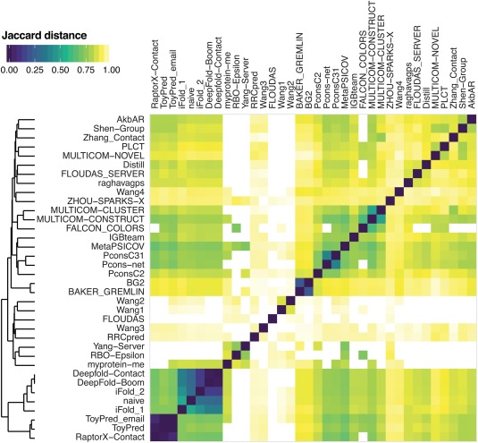
Color‐coded similarity matrix with a dendrogram on the left illustrating the similarity among different methods as judged by the number of common predicted contacts for all targets. The Jaccard distances used in the matrix are calculated on the union of the predicted top L/2 medium‐ and long‐range contacts for each pair of groups

Table 1.

Brief description of the methods participating in CASP12 contact prediction according to the CASP12 Abstracts (http://predictioncenter.org/casp12/doc/CASP12_Abstracts.pdf) if available

Methods	Group ID	Remarks
AkbAR	G389	A meta‐classifier combining several distinct approaches used for inferring contacts from multiple sequence alignments along with a broad range of sequence‐derived features
BAKER_GREMLIN30 BG2	G030, G157	A pseudo‐likelihood‐based method using co‐evolution information from multiple sequence alignments
Deepfold‐Contact, iFold_1, naive	G219, G079, G109	Deep learning‐ based contact prediction algorithms using amino acid composition from the MSA, secondary structure predicted by PSIPRED,50 solvent accessibility predicted by SOLVPRED,31 and co‐ evolutionary patterns by CCMPred51 and EVfold.45 MSAs were generated using HHBlits52 and JackHMMER53 for the full sequence (ifold_1, naive) or predicted domains (Deepfold‐Contact)
Distill	G407	A system based on 2D‐ Recursive Neural Networks with sequence; MSA; PSI‐BLAST,54 SAMD and SAMD templates as input data.
FALCON_COLORS	G348	An approach predicting contacts by removing background correlations via low‐rank and sparse decomposition of a residue correlation matrix. The matrix is calculated by using local statistical models (e.g., MI and OMES) or global statistical models (e.g., mfDCA34 and PSICOV32).
FLOUDAS FLOUDAS_SERVER	G040, G357	The prediction of tertiary contacts is based on the integration of a random forest model that utilizes coevolution scores and sequence‐based features, and tertiary contacts extracted from the structural templates identified by conSSert55/HHsuite.56
IGBteam	G310	Deep learning approach combining evolutionary information, co‐evolution information, CCMpred51 and FreeContact25 predictions, and predicted secondary structure and relative solvent accessibility using SSpro and ACCpro.57
MetaPSICOV31	G013	A neural network‐based method inferring coevolutionary signals from multiple sequence alignments of three distinct approaches (PSICOV,32 DCA/FreeContact,25 CCMpred51). It also considers a broad range of other sequence derived features including secondary structure, solvent accessibility as well as a range of metrics describing both the local and global quality of the input MSA (generated using HHBLITS52)
MULTICOM‐CLUSTER	G287	a meta‐predictor that combines contacts predicted by the two other methods—CONSTRUCT and NOVEL
MULTICOM‐CONSTRUCT	G236	A predictor employing MetaPSICOV31 contact prediction with custom MSAs generated with HHblits52 and JackHMMER58
MULTICOM‐NOVEL (DNcon59)	G345	A sequence‐based deep learning contact predictor.
Myprotein‐me (plmConv)	G251	A method using a deep, convolutional neural network relying on the evolutionary coupling inference of a Potts model, using pseudolikelihood maximization26 and a single multiple sequence alignment generated with jackHMMer.
Pcons‐net, PconsC2, PconsC31	G432, G024, G097	A deep learning approach combining PSICOV32 and plmDCA26 predictions built on eight different HHblits52 and jackHMMer53 alignments. PconsC2 analyses the predictions in context of neighboring residue pairs. Pcons31 includes a non‐DCA contact prediction method and selects the best of eight input alignments.
PLCT	G281	A neural network method that has been trained using unbalanced training, oversampling the negative class. The training set has been built based on predicted solvent accessibilities and predicted secondary structures.60
raghavagps (RRCpred2)	G320	A simple method that utilizes predicted tertiary structures of a protein for identification of residue‐residue contacts. After ranking predicted structures using quality assessment software QASproCL, residue‐residue contacts are determined in the top 10 protein structures based on distance between residues. From these, residue‐residue contacts are predicted for the target protein based on consensus/average.61
RaptorX‐Contact	G451	A deep learning method predicting contacts by integrating both evolutionary coupling and sequence conservation information through an ultra‐deep residual neural network
RBO‐Epsilon	G020	A deep learning method combining evolutionary, sequence‐based, and physicochemical information stemming from EPC‐map46
RRCpred	G108	A model using the Logistic classifier of WEKA62
Shen‐Group	G431	Updated version of R2C63 predicting residue contacts by fusing multiple base predictors composed of both Machine learning‐based and correlated mutation analysis‐based (mfDCA,34 PSICOV,32 and GREMLIN30) approaches. Noise reduction is applied to the CMA‐based predictions.
Wang1–4	G132, G206, G458, G195	Methods trained on a set of features including PSIPRED50 and ACCpro64 predictions using support vector machines,65 direct coupling analysis34 and stacked denoising autoencoders
Yang‐Server	G044	A Pipeline by combining existing contact prediction methods including SVMSEQ,66 BETAcon,67 DNcon,59 CCMpred,51 MetaPSICOV,31 and PconsC222 with template‐based modeling using the I‐TASSER Suite.68
Zhang_Contact (NN‐BAYES)	G373	A neural network combining the contact prediction from three machine‐learning methods (BETACON,67 SVMCON,69 and SVMSEQ66), three coevolution methods (mfDCA,25 PSICOV,32 and CCMpred51), and two meta‐server methods (STRUCTCH70 and MetaPSICOV,31 using the naive Bayes classifier (NBC) with a set of intrinsic sequence‐based features.
ZHOU‐SPARKS‐X	G452	A probabilistic‐based matching approach71

In CASP11, the use of evolutionary coupling data in contact prediction had started to gain traction by significantly improving the predictive power, mostly due to a better distinction of covariance signals from indirect effects.10 As a consequence, one of the groups that was actively pushing this methodology forward—the David Jones' group from the UCL, outperformed the other CASP11 groups with their MetaPSICOV31 method. While the average precision of the best predictor in CASP11 showed a significant increase from 21% to 27% compared to CASP10, it almost doubled in CASP12 with the top predictor reaching an average precision of 47% on the L/5 long‐range contacts for the 38 FM domains (Figure 2). This is an impressive improvement with respect to the previous CASP rounds. Within the reduced lists, the maximum recall achievable was limited based on the number of true contacts and the sequence length. For the L/5 list the highest recall by target varies between 3% and 15%, and for the L/2 lists between 5% and 35%.

Figure 2.

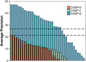
Average precision of long range contacts on L/5 lists for free modeling targets in CASP10 (red), CASP11 (green), and CASP12 (blue) sorted by rank. Grey dashed lines indicate the levels of the best performing group in CASP10 and CASP11, respectively. While only one group showed a significantly better average precision than all the others in CASP 11 compared to CASP10, 26 groups showed an improved average precision in CASP12 compared to the best performing group of CASP11

In contrast to CASP11, where one group was clearly at the top and there was a big separation between the top group and the rest, in CASP12 several methods achieved comparable high accuracy performance, with 12 groups reaching a precision above 40%, and 26 showing a better performance than the best performing method in CASP11. Precisions above 90% in the L/5 list of medium and long‐range contacts were reached for almost half of the targets (Figure 3), and the perfect precision of 100% was reached for six targets on the L/5 and one target on the L/2 list. In general, the average precision of the best performing groups ranges between ∼35% (long range contacts, L/2, FM targets only) up to ∼70% (medium + long range contacts, L/5, FM + FM/TBM targets), which is significantly higher than in previous CASP experiments.

Figure 3.

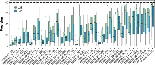
The Precision distribution of medium and long range contacts within the L/2 (blue) and L/5 (green) set for increasing levels of alignment depth (specified in parentheses) in the FM category. Precisions above 90% were reached for almost half of the targets in the L/5 list

The main driver for the improved prediction performance seems to be the usage of coevolution data. To verify this, we assessed the correlation of the precision with alignment depth of each target. Both the average precision by target and the precision of the five groups with the highest values on average show a strong correlation with the alignment depth (log(AlignDepth)∼Prec: R ² = ∼0.56) suggesting that coevolution data are indeed the main driver of the improved quality of contact prediction (Figure 4A and Supporting Information Figure S1). While a minimum number of 0.3 to 1 non‐redundant sequences per residue was suggested to be the cutoff to effectively use coevolution data,16, 45, 46 good predictions with precision above 50% are observed at alignment depths around L/10 already. Unlike the alignment depth, the sequence length does not appear to have a significant effect (R ² = ∼0.03) on the prediction performance (Figure 4B).

Figure 4.

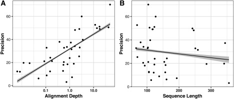
Plot of average precision by target for all groups versus (A) alignment depth (logarithmic scale) for the FM targets and (B) sequence length. While a correlation between precision and alignment depth can be observed (R ²∼0.56), there is no significant correlation between the sequence length and precision (R ² ∼0.03)

3.1. Assessing the information content

While the precision is a good measure to evaluate the reliability of a prediction, it does not necessarily reflect the usefulness of the prediction especially when considering reduced lists of the L/2 and L/5 size. With the number of medium and long range contacts of the targets being between one and two times the sequence length (Supporting Information Figure S2), predictions in the reduced lists cover at most 50% of the available contacts. In consequence, predicted contacts might cluster and solely provide information on a sub‐region of the sequence.

To assess the information content of the correctly predicted contacts we thus used the entropy score (ES—see Materials and Methods), which, as described above, assesses the information content of the contacts by measuring how much they reduce the entropy and thus the conformational space of the protein. Figure 5 shows that the measure is indeed effective in distinguishing whether predictions cluster in sub‐regions or spread across all true contacts.

Figure 5.

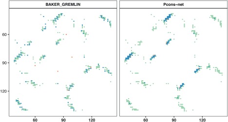
Contact maps for two distinct predictions of L/2 medium and long range contacts for target T0866. Both predictions have an identical precision of 94.23% but a quite a different distribution of contacts with the true predictions (blue) on the left‐hand side spreading equally over the true contacts (green and blue) while on the right‐hand side the predicted contacts cluster in three different regions. This is reflected in a difference in Entropy score of 19.1 for BAKER_GREMLIN and 14.1 for Pcons‐net

Yet, similar to the precision, the entropy score captures only the effect of correctly predicted contacts and is thus not only correlated to the dispersion of contacts but also the number of those contacts in the prediction, which has implications for its information content. Specifically, for full lists, the maximum performance can be achieved by simply predicting all residues to be in contact. Therefore, it is only meaningful to use the entropy score as an additional measure to compare groups with otherwise similar performance in terms of precision or F1 measures (see Figure 5).

3.2. Structure prediction using contacts

To test the real impact of predicted contacts on structure prediction, we used the contact predictions to complement the AbinitioRelax protocol of the widely used Rosetta software suite.37 We only considered single domain targets (14 in total). Contacts were implemented in a fashion that penalized violation of a provided restraint. It has been shown that a small set of distance restraints can significantly improve the performance of de novo structure predictors.47 When using contact predictions, a larger set of restraints might however be beneficial to compensate for false positive predictions within the restraint set. Raptor‐X for example uses lists with 2–3 L contacts coupled to the associated probabilities for structure generation.16, 48 Using contact predictions for five list sizes, coming from 32 groups and using Rosetta without any restraints as a reference, we generated 2.630.000 Rosetta models, which we then compared to the corresponding reference structures.

An improvement in GDT_TS could be observed for most targets (Figure 6). The highest achieved GDT_TS values considering all generated models for each of the 14 domains ranged from 11 to 63 (T0878/T0862) for predictions without contact information, and 12 to 70 (T0941/T0862) for predictions using contact information. Considering only the best five structures by score the highest GDT_TS for modeling without contacts drops to 45 while the one with predicted contact restraints remains at 70, demonstrating that the contact information can improve the ranking of models. An example of the improved structure prediction for target T0915 is shown in Figure 7. Based on the superposition it is apparent that the contact‐assisted prediction matches the fold of the target nicely while in the unguided model three of the eight helices are shifted substantially in respect to the target structure.

Figure 6.

Effect of alignment depth (x axis) and target length (gradient) on overall GDT_TS (A) and GDT_TS improvement (Δbest GDT_TS—B). An overall poor GDT_TS (A) is observed for the longest targets (white and light gray) regardless of alignment depth. The smallest changes in best GDT_TS are observed for the targets with an alignment depth below 0.05 (B)

Figure 7.

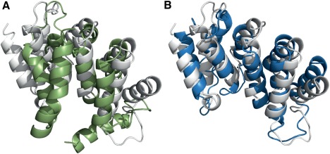
Improvement in Modeling for target T0915; while the best model from the run without restraints (green) reaches a GDT_TS of only 35 (A) to the reference structure (white), the best model from the run with restraints (blue) reaches a GDT_TS of 52 (B)

In general, the overall best GDT_TS was poorer for larger targets (>250 amino acids). The improvement in GDT_TS compared to modeling without restraints was least pronounced in targets with an alignment depth below 0.05 (Figure 6). This might be a result of the poorer performance of contact prediction on targets with shallow sequence alignments.

We analyzed how the precision and size of the used contacts lists affect the best GDT_TS of the resulting models. This revealed a clear correlation between precision and the best GDT_TS for most targets. However, the effects vary widely for different targets and list sizes. While all predictions with precisions above 60% are associated with an improvement of the best GDT_TS in target T0904 (above the level of the unrestrained run indicated by the dashed line), several predictions with precisions close to 100% show only moderate to no improvement for target T0866 (Figure 8). In general, a beneficial effect of using contacts can be seen for most targets in sampling (more structures are closer to the native conformation—Supporting Information Figure S3) and scoring (Figure 8 and Supporting Information Figure S4).

Figure 8.

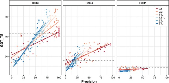
The GDT_TS of contact‐guided Rosetta models built by us for different contact prediction groups as a function of the precision of underlying contact prediction on three representative targets—T0866, T0904 and T0941. The tertiary structure predictions were built separately for six lengths of contact lists (0.2–3 L) used to guide the modeling. Points in the graph represent the highest GDT_TS score within the top five structures built for each contact prediction group. The best GDT_TS of the Top five models without contacts is indicated by the dashed vertical line. In general, the best GDT_TS correlates with the precision. Hardly any improvement in respect to the run without constraint is observed for T0941 (right). While Precisions above 50% are associated with an increased best GDT_TS for target T0904 (middle), even precisions of 100% are not resulting in an improved best GDT_TS in all cases in T0866 (left)

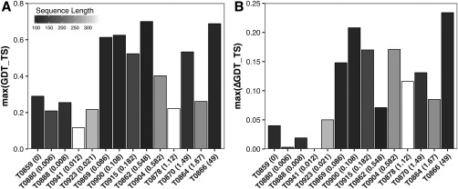
No definite answer can be drawn regarding the best number of contacts to use for modeling. For target T0866, the largest improvement for five of the best performing groups was observed for list sizes between 0.5 and 2 L, with even list sizes of 3 L resulting in improvement in two out of five cases (Figure 9). Considering the predictions of the 20 best groups on the seven targets with GDT_TS > 30, list sizes of L/5 or L/2 appear to be the best choice.

Figure 9.

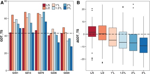
(A) Effect of the number of employed contacts on the improvement of GDT_TS within the top five models by score. Performance of the run without restraints is indicated by the dashed line. For the best five ranked groups (ranking according to Table 2) the list size with the biggest improvement varies between L/2 to 2*L for target T0866. (B) In contrast the best option based on the boxplot for the top 10 groups (ranking according to Table 2) on the seven targets with a GDT_TS above 30 is L/5 with a slight margin over L/2

The performance is apparently also dependent on the submitted contact lists: while L/2 predictions of some groups improve the best GDT_TS for six of the seven targets, others improve only in one of the seven cases (Figure 10). Interestingly the two groups with the most pronounced improvement in this category (PconsC31 and raghavagps) are not within the five best groups of the L/2‐based ranking (see Table 2). Also, predictions of iFold_1 and DeepFold‐contact (G079 and G219), which are among the best performing groups in the L/2 ranking, do not improve best GDT_TS in most of the tested cases.

Figure 10.

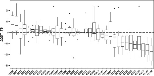
Distribution of delta GDT_TS values by group compared to the modeling without restraints for the best GDT_TS within the top five structures by score over all targets reaching ΔGDT_TS values above 25 (L/2 medium‐range and long‐range contacts). Interestingly groups performing well in the L/2 ranking in Table 2 like G079 and G219 (underlined) have a lower GDT_TS in the majority of targets compared to the reference, groups that are not in the Top 5 (G097 and G320) of the ranking show on average the biggest improvement in GDT_TS

Table 2.

z‐scores ranking based on the sum of z‐scores for various measures and list sizes covering reduced lists (L/2 and L/5) and the full prediction (FL)^a

	L/2	L/5		Full List			Average rank ± SD
	F1+	Prec		F1+	MCC+	AUC_PR
	0.5*ES	—	—	0.5*ES	0.5*ES	—
RaptorX‐Contact	1	1	1	4	2	1	1.7 ± 1.2
MetaPSICOV	2	2	2	15	12	3	6.0 ± 5.9
iFold_1	3	4	8	3	1	2	3.5 ± 2.4
MULTICOM‐CONSTRUCT	4	3	3	13	10	5	6.3 ± 4.2
RBO‐Epsilon	5	5	4	18	15	6	8.8 ± 6.0
Deepfold‐Contact	6	8	11	5	4	4	6.3 ± 2.7
FALCON_COLORS	7	6	7	19	16	8	10.5 ± 5.5
Yang‐Server	8	7	5	17	18	10	10.8 ± 5.4
AkbAR	9	14	15	22	21	15	16.0 ± 4.8
raghavagps	10	11	12	10	9	7	9.8 ± 1.7
Pcons‐net	11	9	6	14	13	9	10.3 ± 2.9
naive	12	13	16	6	6	13	11.0 ± 4.1
Shen‐Group	13	15	13	1	3	14	9.8 ± 6.1
IGBteam	14	10	9	9	7	11	10.0 ± 2.4
PconsC31	15	12	10	16	17	12	13.7 ± 2.7
MULTICOM‐CLUSTER	16	16	14	8	8	17	13.2 ± 4.1
MULTICOM‐NOVEL	17	18	17	2	5	16	12.5 ± 7.1
Zhang_Contact	18	17	19	20	20	18	18.7 ± 1.2
PLCT	19	19	18	26	26	20	21.3 ± 3.7
PconsC2	20	20	20	28	27	21	22.7 ± 3.8
Distill	21	21	21	21	22	19	20.8 ± 1.0
ZHOU‐SPARKS‐X	22	23	28	—	—	29	25.5 ± 3.5
FLOUDAS_SERVER	23	22	23	27	28	22	24.2 ± 2.6
Wang4	24	26	25	—	—	31	26.5 ± 3.1
BG2	25	29	24	24	23	24	24.8 ± 2.1
BAKER_GREMLIN	26	30	22	25	24	23	25.0 ± 2.8
Wang2	27	24	27	—	—	27	26.2 ± 1.5
myprotein‐me	28	25	26	30	30	26	27.5 ± 2.2
RRCpred	29	28	29	12	14	25	22.8 ± 7.8
Wang3	30	27	30	11	19	28	24.2 ± 7.6
Wang1	31	31	32	7	11	32	24.0 ± 11.7
FLOUDAS	32	32	31	23	25	30	28.8 ± 3.9

The table includes rankings of the groups according to the scores illustrated in Figure 13 (see the caption to Figure 13 for details).

Interestingly, the improvement in GDT_TS in the top five models is on average higher if the models predicted with lists of the top5 predictors are pooled and ranked based on their Rosetta score (Supporting Information Figure S5).

In an attempt to assess the capability of the predictions to restrain the conformational search space during structural modeling we calculated the entropy score. However, as mentioned earlier, the ES score, which is calculated only on true positive contacts, is therefore correlated with their number in the predicted contact list. As a result, the plot of the entropy score and GDT_TS is similar to that of precision and GDT_TS (Figure 8 and Supporting Information Figure S3 + 4) with a tendency toward an improved GDT_TS with higher ES values (data not shown). In the structure modeling performed here, we did include the false positive contacts as well, which of course affects the quality of the generated models. The detrimental effects of those false predictions can be seen in the degree of violation (Supporting Information Figure S6). To truly determine the effect of the distribution of contacts as measured by the entropy score, structure modeling neglecting all false positive predictions with an identical number of true contacts but different dispersion along the sequence would be required, which is outside the scope of this work.

In conclusion, contact predictions are a valuable addition to structure prediction as demonstrated in our analysis and confirmed by various other groups as well.16, 28, 30, 47 Surprisingly, performance based on the L/2 contact lists did not directly translate into improvement in GDT_TS when considering all generated models. However, we do observe a clear improvement in the ranking of models. We should also note here that this evaluation was only performed on 14 of the 38 FM domains from which 7 were dropped due to poor overall performance in terms of GDT_TS. The sampling was also limited to only 1000 models generated using the coarse‐grained stage of the AbinitoRelax protocol. Furthermore, the contact predictions, being true or false positive, were incorporated in a stringent manner so the detrimental effect of false positive predictions might outweigh the beneficial effect of the true contacts as indicated by the negative correlation of average restraint violation and GDT_TS improvement (Supporting Information Figure S6). Several different approaches to deal with these issues have been put forward including using for example, the probabilities to weigh or randomly remove contacts,16 use potentials that reward satisfied contacts instead of penalizing violated ones, and various others. Ultimately the best contact prediction method and number of contacts to use will depend on the structure prediction method and the way contacts are incorporated into the modeling.

3.3. Group performances on various measures and list sizes

With structure prediction being the most prominent use case for predicted contacts, the most relevant lists to users are most likely reduced lists of a fixed size. Our analysis of the usefulness of contacts for structure prediction (see previous section) revealed that the highest improvement in GDT_TS is mostly observed in the lists larger than L/5. Consequently, we decided to focus evaluation of group performance on the L/2 lists. Still, the rankings on the L/2 and L/5 lists are rather similar as seen for example, for the average precision based ranking (Figure 11). A pairwise t test for the precision on L/2 lists for all groups shows that, unlike in CASP11, no single predictor performs significantly better than all the others but that the best performing top 10 groups have a rather similar performance (Figure 12).

Figure 11.

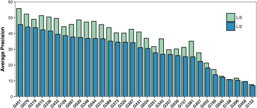
Average Precision by group for the L/2 and L/5 list (medium and long range contacts, FM targets). While the average precision of the L/5 predictions is in most cases slightly higher than the L/2 precision, the ranking on either metric will be similar

Figure 12.

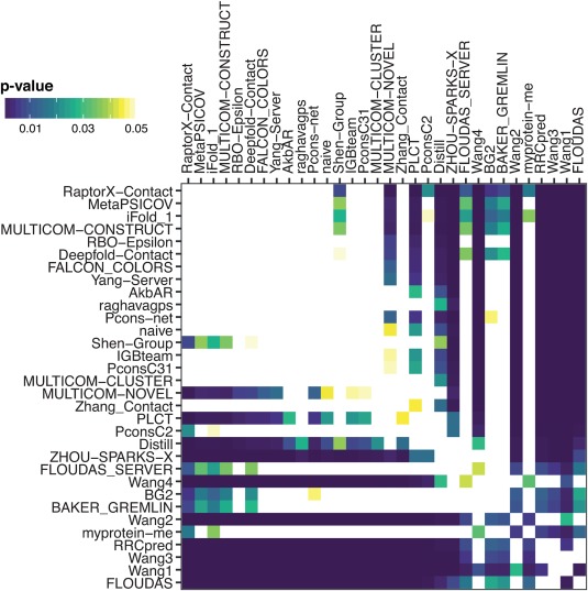
Paired t test comparing average precision (L2/FM/ML) per target for each of the 32 groups. P values <0.05 are shaded indicating a significant difference between the groups. White indicates no significant difference between the groups while darker shades represent higher significance. Based on the matrix, there is no significant difference between the predictions of the best performing groups

For final ranking of groups, we chose to use the F1 + 0.5*ES formula. The F1 score holds the main weight in the ranking, rewarding groups who correctly predict larger number of native contacts, while maintaining higher percentage of correct contacts in their predictions. The entropy score (ES) is included with a smaller weight, giving additional advantage to groups with higher information content (that is, larger spread) of the predicted contacts. Groups in Figure 13A are ordered according to the final score (the leftmost bars in dark blue color). The panel A also includes ranks of the groups solely based on the precision for the L/2 and L/5 lists (similar to CASP11) as well as the rank on the full‐list AUC_PR measure, which was previously introduced to assess the overall ranking capability of the predictors.10 Ranking based on the combined measure (F1 + 0.5*ES) is very similar to that solely based on precision, which is identical to a ranking solely based on F1 for reduced lists. This indicates that the addition of the new measure does not drastically alter the ranking but slightly favors predictors with a broader distribution of the predicted true contacts.

Figure 13.

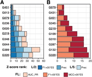
Top 10 predictors by cumulative z‐scores on (A) metrics assessing ranking of probabilities and (B) metrics assessing binary contact classification based on the 0.5 cutoff according to the assessor‐selected scores in each category. The four predictors appearing in the top 10 of both rankings are underlined. The scores in panel A include three reduced list scores—the F1 + 0.5*ES combination of the F1 and entropy scores, and the precision on L/2 and L/5 data, and one full list score—the area under the curve in the precision‐recall analysis (AUC_PR). The scores in panel B include the F1 + 0.5*ES and MCC + 0.5*ES combinations of the F1, MCC and the entropy scores. For the FL assessment of MCC and F1, only the residue pairs predicted with the probability >0.5 were considered as contacts. The results in panel (B) are therefore affected by the way some groups scaled their contacts, not submitting predictions with probabilities above 0.5 for several targets

We also performed the analysis based on the F1, MCC and ES scores for full contact predictions using the probability of 0.5 for separating contacts from non‐contacts, thus determining the performance of the predictors as binary classifiers assigning probabilities above 0.5 to true contacts. The results of this analysis are presented in Figure 13B. As one can see, the composition and order of groups in both panels are very different, which tells us that some of the highest ranked groups in panel A (like G013 or G236) are not that successful in assigning probabilities >0.5 to their correct predictions. Data for all groups on all scores are presented in Table 2.

3.4. Significance of contact probabilities

While in the above measures, the probabilities submitted with the contacts are only used to rank the predictions for generation of the reduced lists, or as binary classifier in form of the 0.5 cutoff, the probability can hold more information and should ideally reflect with what certainty the predicted contact is indeed a true contact. Similar to previous CASP experiments, the submissions of groups were very diverse in respect to the number of contacts submitted and the distribution of the associated probabilities. Some groups submitted only a few contacts while others predicted almost the entire matrix to be in contact with a probability >0.5. Despite the instructions that 0.5 will be used to distinguish contacts from non‐contacts, few groups even submitted predictions with almost no contacts above that threshold (Figure 14).

Figure 14.

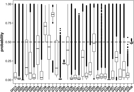
Boxplot showing statistics on the contact probabilities submitted FM and FM/TBM targets for CASP12. One group submitted only confident contacts (G108), while others did not appear to take the requested format into consideration by submitting almost all the contacts with probabilities below 0.5 (e.g., G206 and G458)

To determine whether the submitted probabilities reflect indeed the likelihood that the predicted contact is a true contact we determined the fraction of true positives for several probability intervals (Figure 15). While the correlation was poor for a few groups, most, but not all, of the best performing groups provided meaningful probabilities. Of course, the correlation was target dependent with probabilities showing a perfect correlation to the fraction of TP on some targets and no correlation on others (data not shown).

Figure 15.

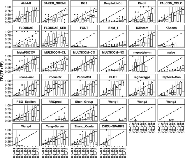
boxplots per group depicting the fraction of True Positive contacts for the 10 intervals between 0 and 1 (step = 0.1). The perfect correlation between the intervals and the true positive fraction of the prediction (TP/[TP + FP]) is indicated by the dashed line. In the majority of groups TP/[TP + FP] corresponds roughly to the probability interval

Still the results are encouraging and suggest that probabilities are indeed the values to be considered when using the predicted contacts for structure calculation.

4. CONCLUSIONS

While CASP11 saw the advent of evolutionary couplings in contact prediction, in CASP12 these methods matured mostly by coupling the coevolution information with machine learning. Some predictors indicate that improved methodology including deeper networks is one of the main drivers for the significant improvement in predictions.48, 49 Another reason for the enhanced performance in CASP12 appears to be the increase in the number of sequences available (Figure 16) and, thus, the evolutionary information that can be extracted. Thus, the combination of the increase in sequence database size together with the widespread adoption of evolutionary couplings in conjunction with deep learning seems to be at the origin of the increased performance of more than half the predictors compared to the best predictor in CASP11. No single group stands out significantly from the other in the top10.

Figure 16.

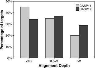
Distribution of sequence depth over all targets for CASP11 (white light gray) and CASP12 (black) for targets with low (<0.5), medium (0.5‐2), and high alignment depth. Alignment depth values were calculated from the outputs of HHblits and PSI‐BLAST as described previously10 using the latest databases available after closure of the prediction window for each target

With the significant improvement in predicting inter‐residue contacts, their incorporation in a sensible and efficient way into structure prediction workflows remains the main challenge. This is an area under active development with several approaches already using contact prediction in distinct manners.16, 28 As demonstrated, various factors can affect the performance of the structure modeling, including the number of contacts used and the way the contacts are used in the protocol. Another relevant aspect is the way the probabilities are defined and used. While CASP assessment so far mostly focused on ranking and binary classification, Figure 15 shows that the actual probabilities hold valuable information that can be incorporated into the modeling approaches. It remains thus to be seen how the observed major increase of the predictive power in contact prediction will translate into further improvements in de novo structure prediction within the coming years.

Supporting information

Additional Supporting Information may be found online in the supporting information tab for this article.

Supporting Information

Schaarschmidt J, Monastyrskyy B, Kryshtafovych A, Bonvin AMJJ. Assessment of contact predictions in CASP12: Co‐evolution and deep learning coming of age. Proteins. 2018;86:51–66. https://doi.org/10.1002/prot.25407

REFERENCES

- 1. Lesk AM. CASP2: report on ab initio predictions. Proteins. 1997;(suppl1):151–166. [DOI] [PubMed] [Google Scholar]
- 2. Orengo CA, Bray JE, Hubbard T, LoConte L, Sillitoe I. Analysis and assessment of ab initio three‐dimensional prediction, secondary structure, and contacts prediction. Proteins. 1999;(suppl3):149–170. [DOI] [PubMed] [Google Scholar]
- 3. Lesk AM, Conte Lo L, Hubbard TJ. Assessment of novel fold targets in CASP4: predictions of three‐dimensional structures, secondary structures, and interresidue contacts. Proteins. 2001;45(suppl 5):98–118. [DOI] [PubMed] [Google Scholar]
- 4. Aloy P, Stark A, Hadley C, Russell RB. Predictions without templates: new folds, secondary structure, and contacts in CASP5. Proteins. 2003;53(suppl 6):436–456. [DOI] [PubMed] [Google Scholar]
- 5. Graña O, Baker D, MacCallum RM, et al. CASP6 assessment of contact prediction. Proteins. 2005;61(suppl 7):214–224. [DOI] [PubMed] [Google Scholar]
- 6. Izarzugaza JMG, Graña O, Tress ML, Valencia A, Clarke ND. Assessment of intramolecular contact predictions for CASP7. Proteins. 2007;69(suppl 8):152–158. [DOI] [PubMed] [Google Scholar]
- 7. Ezkurdia I, Graña O, Izarzugaza JMG, Tress ML. Assessment of domain boundary predictions and the prediction of intramolecular contacts in CASP8. Proteins. 2009;77(suppl 9):196–209. [DOI] [PubMed] [Google Scholar]
- 8. Monastyrskyy B, Fidelis K, Tramontano A, Kryshtafovych A. Evaluation of residue‐residue contact predictions in CASP9. Proteins. 2011;79(suppl 10):119–125. [DOI] [PMC free article] [PubMed] [Google Scholar]
- 9. Monastyrskyy B, D'andrea D, Fidelis K, Tramontano A, Kryshtafovych A. Evaluation of residue‐residue contact prediction in CASP10. Proteins. 2014;82(suppl 2):138–153. [DOI] [PMC free article] [PubMed] [Google Scholar]
- 10. Monastyrskyy B, D'andrea D, Fidelis K, Tramontano A, Kryshtafovych A. New encouraging developments in contact prediction: assessment of the CASP11 results. Proteins. 2016;84(suppl 1):131–144. [DOI] [PMC free article] [PubMed] [Google Scholar]
- 11. Saitoh S, Nakai T, Nishikawa K. A geometrical constraint approach for reproducing the native backbone conformation of a protein. Proteins. 1993;15(2):191–204. [DOI] [PubMed] [Google Scholar]
- 12. Bohr J, Bohr H, Brunak S, et al. Protein structures from distance inequalities. J Mol Biol. 1993;231(3):861–869. [DOI] [PubMed] [Google Scholar]
- 13. Skolnick J, Kolinski A, Ortiz AR. MONSSTER: a method for folding globular proteins with a small number of distance restraints. J Mol Biol. 1997;265(2):217–241. [DOI] [PubMed] [Google Scholar]
- 14. Taylor TJ, Bai H, Tai C‐H, Lee B. Assessment of CASP10 contact‐assisted predictions. Proteins. 2014;82(suppl 2):84–97. [DOI] [PMC free article] [PubMed] [Google Scholar]
- 15. Vassura M, Margara L, Di Lena P, Medri F, Fariselli P, Casadio R. FT‐COMAR: fault tolerant three‐dimensional structure reconstruction from protein contact maps. Bioinformatics. 2008;24(10):1313–1315. [DOI] [PubMed] [Google Scholar]
- 16. Wang S, Sun S, Li Z, Zhang R, Xu J. Accurate de novo prediction of protein contact map by ultra‐deep learning model. PLoS Comput Biol. 2017;13(1):e1005324 [DOI] [PMC free article] [PubMed] [Google Scholar]
- 17. Shindyalov IN, Kolchanov NA, Sander C. Can three‐dimensional contacts in protein structures be predicted by analysis of correlated mutations?. Protein Eng. 1994;7(3):349–358. [DOI] [PubMed] [Google Scholar]
- 18. Göbel U, Sander C, Schneider R, Valencia A. Correlated mutations and residue contacts in proteins. Proteins. 1994;18(4):309–317. [DOI] [PubMed] [Google Scholar]
- 19. Burger L, van Nimwegen E. Disentangling direct from indirect co‐evolution of residues in protein alignments. PLoS Comput Biol. 2010;6(1):e1000633–e1000618. [DOI] [PMC free article] [PubMed] [Google Scholar]
- 20. Ovchinnikov S, Kamisetty H, Baker D. Robust and accurate prediction of residue–residue interactions across protein interfaces using evolutionary information. Elife. 2014;3:1061–1021. [DOI] [PMC free article] [PubMed] [Google Scholar]
- 21. Marks DS, Hopf TA, Sander C. Protein structure prediction from sequence variation. Nat Biotechnol. 2012;30(11):1072–1080. [DOI] [PMC free article] [PubMed] [Google Scholar]
- 22. Skwark MJ, Raimondi D, Michel M, Elofsson A, Wei G. Improved contact predictions using the recognition of protein like contact patterns. PLoS Comput Biol. 2014;10(11):e1003889 [DOI] [PMC free article] [PubMed] [Google Scholar]
- 23. Marks DS, Colwell LJ, Sheridan R, et al. Protein 3D structure computed from evolutionary sequence variation. PLoS One. 2011;6(12):e28766–e28720. [DOI] [PMC free article] [PubMed] [Google Scholar]
- 24. Weigt M, White RA, Szurmant H, Hoch JA, Hwa T. Identification of direct residue contacts in protein‐protein interaction by message passing. Proc Natl Acad Sci USA. 2009;106(1):67–72. [DOI] [PMC free article] [PubMed] [Google Scholar]
- 25. Kaján L, Hopf TA, Kalaš M, Marks DS, Rost B. FreeContact: fast and free software for protein contact prediction from residue co‐evolution. BMC Bioinformatics. 2014;15(1):85 [DOI] [PMC free article] [PubMed] [Google Scholar]
- 26. Feinauer C, Skwark MJ, Pagnani A, Aurell E, Dunbrack RL. Improving contact prediction along three dimensions. PLoS Comput Biol. 2014;10(10):e1003847–e1003813. [DOI] [PMC free article] [PubMed] [Google Scholar]
- 27. Skwark MJ, Abdel‐Rehim A, Elofsson A. PconsC: combination of direct information methods and alignments improves contact prediction. Bioinformatics. 2013;29(14):1815–1816. [DOI] [PubMed] [Google Scholar]
- 28. Michel M, Hayat S, Skwark MJ, Sander C, Marks DS, Elofsson A. PconsFold: improved contact predictions improve protein models. Bioinformatics. 2014;30(17):i482–i488. [DOI] [PMC free article] [PubMed] [Google Scholar]
- 29. Ekeberg M, Hartonen T, Aurell E. Fast pseudolikelihood maximization for direct‐coupling analysis of protein structure from many homologous amino‐acid sequences. J Comput Phys. 2014;276:341–356. [Google Scholar]
- 30. Kamisetty H, Ovchinnikov S. Assessing the utility of coevolution‐based residue–residue contact predictions in a sequence‐and structure‐rich era. Proc Natl Acad Sci USA. 2013; 110(39):15674–15679. [DOI] [PMC free article] [PubMed] [Google Scholar]
- 31. Jones DT, Singh T, Kosciolek T, Tetchner S. MetaPSICOV: combining coevolution methods for accurate prediction of contacts and long range hydrogen bonding in proteins. Bioinformatics. 2015;31(7):999–1006. [DOI] [PMC free article] [PubMed] [Google Scholar]
- 32. Jones DT, Buchan DWA, Cozzetto D, Pontil M. PSICOV: precise structural contact prediction using sparse inverse covariance estimation on large multiple sequence alignments. Bioinformatics. 2012;28(2):184–190. [DOI] [PubMed] [Google Scholar]
- 33. Sulkowska JI, Morcos F, Weigt M, Hwa T, Onuchic JN. Genomics‐aided structure prediction. Proc Natl Acad Sci USA. 2012;109(26):10340–10345. [DOI] [PMC free article] [PubMed] [Google Scholar]
- 34. Morcos F, Pagnani A, Lunt B, et al. Direct‐coupling analysis of residue coevolution captures native contacts across many protein families. Proc Natl Acad Sci USA. 2011;108(49):E1293–E1301. [DOI] [PMC free article] [PubMed] [Google Scholar]
- 35. Nabuurs SB, Spronk CAEM, Krieger E, Maassen H, Vriend G, Vuister GW. Quantitative Evaluation of Experimental NMR Restraints. J Am Chem Soc. 2003;125(39):12026–12034. [DOI] [PubMed] [Google Scholar]
- 36. Crippen GM. Rapid calculation of coordinates from distance matrices. J Comput Phys. 1978;26(3):449–452. [Google Scholar]
- 37. Leaver‐Fay A, Tyka M, Lewis SM, et al. ROSETTA3: an object‐oriented software suite for the simulation and design of macromolecules. Meth Enzymol. 2011;487(C):545–574. [DOI] [PMC free article] [PubMed] [Google Scholar]
- 38. Misura KMS, Chivian D, Rohl CA, Kim DE, Baker D. Physically realistic homology models built with ROSETTA can be more accurate than their templates. Proc Natl Acad Sci USA. 2006;103(14):5361–5366. [DOI] [PMC free article] [PubMed] [Google Scholar]
- 39. Zemla A. LGA: a method for finding 3D similarities in protein structures. Nucleic Acids Res. 2003;31(13):3370–3374. [DOI] [PMC free article] [PubMed] [Google Scholar]
- 40. Ortiz AR, Strauss CEM, Olmea O. MAMMOTH (Matching molecular models obtained from theory): an automated method for model comparison. Protein Sci. 2009;11(11):2606–2621. [DOI] [PMC free article] [PubMed] [Google Scholar]
- 41. Thompson J, Baker D. Incorporation of evolutionary information into Rosetta comparative modeling. Proteins. 2011;79(8):2380–2388. [DOI] [PMC free article] [PubMed] [Google Scholar]
- 42. Schrödinger LLC. The PyMOL Molecular Graphics System, Version 1.8. 2015.
- 43. Morin A, Eisenbraun B, Key J, et al. Collaboration gets the most out of software. Elife. 2013;2:e01456 [DOI] [PMC free article] [PubMed] [Google Scholar]
- 44. Levandowsky M, Winter D. Distance between sets. Nature. 1971;234(5323):34–35. [Google Scholar]
- 45. Hopf TA, Schärfe CPI, Rodrigues JPGLM, Green AG, Kohlbacher O, Sander C, Bonvin AMJJ, Marks DS. Sequence co‐evolution gives 3D contacts and structures of protein complexes. Elife. 2014;3:e03430 [DOI] [PMC free article] [PubMed] [Google Scholar]
- 46. Schneider M, Brock O, Zhang Y. Combining physicochemical and evolutionary information for protein contact prediction. PLoS One. 2014;9(10):e108438 [DOI] [PMC free article] [PubMed] [Google Scholar]
- 47. Kim DE, DiMaio F, Yu‐Ruei Wang R, Song Y, Baker D. One contact for every twelve residues allows robust and accurate topology‐level protein structure modeling. Proteins. 2014;82(Web Server issue):208–218. [DOI] [PMC free article] [PubMed] [Google Scholar]
- 48. Wang S, Sun S, Xu J. Analysis of deep learning methods for blind protein contact prediction in CASP12. Proteins. 2017;82(suppl 2):208–211. [DOI] [PMC free article] [PubMed] [Google Scholar]
- 49. Buchan DWA, Jones DT. Improved protein contact predictions with the MetaPSICOV2 server in CASP12. Proteins. 2017;33(17):2684–2686. [DOI] [PMC free article] [PubMed] [Google Scholar]
- 50. McGuffin LJ, Bryson K, Jones DT. The PSIPRED protein structure prediction server. Bioinformatics. 2000;16(4):404–405. [DOI] [PubMed] [Google Scholar]
- 51. Seemayer S, Gruber M, Söding J. CCMpred: fast and precise prediction of protein residue‐residue contacts from correlated mutations. Bioinformatics. 2014;30(21):3128–3130. [DOI] [PMC free article] [PubMed] [Google Scholar]
- 52. Remmert M, Biegert A, Hauser A, Söding J. HHblits: lightning‐fast iterative protein sequence searching by HMM‐HMM alignment. Nat Methods. 2011;9(2):173–175. [DOI] [PubMed] [Google Scholar]
- 53. Finn RD, Clements J, Arndt W, et al. HMMER web server: 2015 update. Nucleic Acids Res. 2015;43(W1):W30–W38. [DOI] [PMC free article] [PubMed] [Google Scholar]
- 54. Altschul SF, Madden TL, Schäffer AA, et al. Gapped BLAST and PSI‐BLAST: a new generation of protein database search programs. Nucleic Acids Res. 1997;25(17):3389–3402. [DOI] [PMC free article] [PubMed] [Google Scholar]
- 55. Kieslich CA, Smadbeck J, Khoury GA, Floudas CA. conSSert: Consensus SVM Model for Accurate Prediction of Ordered Secondary Structure. J Chem Inf Model. 2016;56(3):455–461. [DOI] [PubMed] [Google Scholar]
- 56. Söding J. Protein homology detection by HMM‐HMM comparison. Bioinformatics. 2005;21(7):951–960. [DOI] [PubMed] [Google Scholar]
- 57. Magnan CN, Baldi P. SSpro/ACCpro 5: almost perfect prediction of protein secondary structure and relative solvent accessibility using profiles, machine learning and structural similarity. Bioinformatics. 2014;30(18):2592–2597. [DOI] [PMC free article] [PubMed] [Google Scholar]
- 58. Johnson LS, Eddy SR, Portugaly E. Hidden Markov model speed heuristic and iterative HMM search procedure. BMC Bioinformatics. 2010;11(1):431 [DOI] [PMC free article] [PubMed] [Google Scholar]
- 59. Eickholt J, Cheng J. Predicting protein residue‐residue contacts using deep networks and boosting. Bioinformatics. 2012;28(23):3066–3072. [DOI] [PMC free article] [PubMed] [Google Scholar]
- 60. Markowski G, Grabczewski K, Adamczak R. Oversampling negative class improves contact map prediction. Int J Pharma Med Biol Sci. 2016;5(4):211–216. [Google Scholar]
- 61. Agrawal P, Singh S, Nagpal G, Sethi D, Raghava GPS. Prediction of residue‐residue contacts in CASP12 targets from its predicted tertiary structures. bioRxiv. 2017;192120 [Google Scholar]
- 62. Hall M, Frank E, Holmes G, Pfahringer B, Reutemann P, Witten IH. The WEKA data mining software: an update. ACM SIGKDD Explor Newsl. 2009;11(1):10–18. [Google Scholar]
- 63. Yang J, Jin Q‐Y, Zhang B, Shen H‐B. R2C: improving ab initio residue contact map prediction using dynamic fusion strategy and Gaussian noise filter. Bioinformatics. 2016;32(16):2435–2443. [DOI] [PubMed] [Google Scholar]
- 64. Cheng J, Randall AZ, Sweredoski MJ, Baldi P. SCRATCH: a protein structure and structural feature prediction server. Nucleic Acids Res. 2005;33(Web Server):W72–W76. [DOI] [PMC free article] [PubMed] [Google Scholar]
- 65. Joachims T. Making large‐scale SVM learning practical In: Advances in kernel methods. MIT Press Cambridge; 1998; p 169–184. [Google Scholar]
- 66. Wu S, Zhang Y. A comprehensive assessment of sequence‐based and template‐based methods for protein contact prediction. Bioinformatics. 2008;24(7):924–931. [DOI] [PMC free article] [PubMed] [Google Scholar]
- 67. Cheng J, Baldi P. Three‐stage prediction of protein‐sheets by neural networks, alignments and graph algorithms. Bioinformatics. 2005;21(suppl 1):i75–i84. [DOI] [PubMed] [Google Scholar]
- 68. Yang J, Yan R, Roy A, Xu D, Poisson J, Zhang Y. The I‐TASSER Suite: protein structure and function prediction. Nat Biotechnol. 2015;12(1):7–8. [DOI] [PMC free article] [PubMed] [Google Scholar]
- 69. Cheng J, Baldi P. Improved residue contact prediction using support vector machines and a large feature set. BMC Bioinformatics 2007;8(1):113–119. [DOI] [PMC free article] [PubMed] [Google Scholar]
- 70. Sun H‐P, Huang Y, Wang X‐F, Zhang Y, Shen H‐B. Improving accuracy of protein contact prediction using balanced network deconvolution. Proteins. 2015;83(3):485–496. [DOI] [PMC free article] [PubMed] [Google Scholar]
- 71. Yang Y, Faraggi E, Zhao H, Zhou Y. Improving protein fold recognition and template‐based modeling by employing probabilistic‐based matching between predicted one‐dimensional structural properties of query and corresponding native properties of templates. Bioinformatics. 2011;27(15):2076–2082. [DOI] [PMC free article] [PubMed] [Google Scholar]
Associated Data
This section collects any data citations, data availability statements, or supplementary materials included in this article.
Supplementary Materials