

Abstract
Current protein classification methods treat high-resolution structures as static entities. However, experiments have well documented the dynamic nature of proteins. With knowledge that thermodynamic fluctuations around the high-resolution structure contribute to a more physically accurate and biologically meaningful picture of a protein, the concept of a protein’s energetic profile is introduced. It is demonstrated on a large scale that energetic profiles are both diagnostic of a protein fold and evolutionarily relevant. Development of Structural Thermodynamic Ensemble-based Protein Homology (STEPH), an algorithm that searches for local similarities between energetic profiles, constitutes a first step towards a long-term goal of our laboratory to integrate thermodynamic information into protein-fold classification approaches.
1. Introduction
Fold classification is indispensable for rationalizing evolutionary relationships between proteins (Kinch and Grishin, 2002; Lecomte et al., 2005; Russell, 2002). Many classification schemes exist, each organizing fold space from different viewpoints (Finn et al., 2008; Greene et al., 2007; Heger et al., 2007; Kriventseva et al., 2001; Murzin et al., 1995; Shindyalov and Bourne, 2000; Tatusov et al., 2003). Classification can be based on criteria including sequence, structure, or function, with the most useful schemes integrating information from several sources and supplemented by expert curation. Naturally, schemes based on different criteria exhibit differences in classification (Alva et al., 2008; Day et al., 2003; Kolodny et al., 2006; Taylor, 2007). These differences sometimes result in conflicting biological interpretations.
It is our hypothesis that a subset of the differences between classification schemes is caused by neglect of a fundamental property of proteins; namely, that proteins exhibit dynamic fluctuations. Fluctuations are amply documented by experiment (Henzler-Wildman and Kern, 2007; Igumenova et al., 2006; Mittermaier and Kay, 2006) and indicate the presence of an ensemble of conformations under physiological conditions. Thus, the biologically relevant character of even the most stable proteins is most accurately described by the formalism of statistical thermodynamics. However, all current classification schemes that we are aware of ignore the energetic and dynamic variations within individual proteins, treating each high-resolution structure as merely a single rigid entity out of the billions of conformers sampled by each protein. At best, this treatment results in an incomplete understanding of fold space. At worst, it is possible that important evolutionary relationships, based on shared energetic patterns, are overlooked or incorrect.
Integration of dynamic information into protein-fold classification schemes is a long-term goal of our laboratory. Through a combination of proven algorithms and emerging methodology, two initial steps have now been achieved. First, detailed descriptions of local energetics have been calculated for a sampling of the complete protein-fold space. These descriptions are termed “energetic profiles” of proteins. Second, it has become clear that energetic profiles are thermodynamic fingerprints, diagnostic of a protein fold without regard to sequence, structure, or functional information. Interestingly, energetic profiles often, but not always, complement such information. Therefore, energetic profiling of fold space has become crucial to development of a future evolutionary classification scheme integrating sequence, structure, and function with thermodynamic information. It is hoped that such a classification will ultimately reconcile differences in existing schemes and lead to a greater understanding of principles of protein structure and mechanisms of protein evolution.
2. Modeling the Native State Ensemble of Proteins using Statistical Thermodynamics
The energetic profile of a protein is defined by thermodynamic properties as a function of residue position (Fig. 11.1). In contrast to the more common sequence-based profile of a protein family, which contains only amino acid frequencies (Dunbrack, 2006), an energetic profile may contain one or more thermodynamic properties, such as Gibbs free energy of stability, enthalpy, and entropy. These properties can be determined experimentally for individual proteins in favorable cases, for example, by NMR-detected hydrogen exchange (Ferreon et al., 2003; Milne et al., 1999; Orban et al., 1995). However, it is difficult to obtain experimental measurements on large numbers of proteins. Therefore, energetic profiling of fold space demands a computational approach.
Figure 11.1.
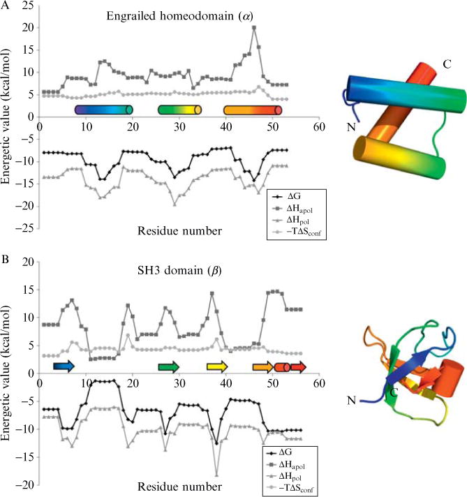
Energetic profiles of three diverse protein structures. These profiles consist of local stability (ΔG), apolar solvation enthalpy (ΔHapol), polar solvation enthalpy (ΔHpol), and conformational entropy (−TΔSconf). The COREX algorithm (window size 5 residues, minimum window-size 4 residues, entropy weighting factor 0.5, simulated pH of 7.0, temperature 25.°C) was run on three proteins: (A) drosophila engrailed homeodomain (PDB code 1p7iA, SCOP sid d1p7ia, SCOP structural class all-alpha, a.4.1.1), (B) mouse SH3 domain (PDB code 1ckaA, SCOP sid d1ckaa1, SCOP structural class all-beta, b.34.2.1), (C) human class sigma glutathione S-transferase, N-terminal domain (PDB code 1iyhA, SCOP sid d1iyha2, SCOP structural class alpha/beta, c.47.1.5). DSSP secondary structure(Kabsch and Sander, 1983) is indicated immediately above the x-axis, helices as cylinders and strands as arrows. Rainbow colors indicate progression from N to C terminus to aid in the reader’s mapping of locations along the primary sequence to locations in the tertiary structure. All energetic values vary as a function of location in the protein structure, a result observed by experiment but not anticipated by treatment of the structure as a rigid entity.
Our approach is to model the native state ensemble of a protein using statistical thermodynamics (Hilser, 2001; Hilser et al., 2006). The basic recipe is as follows: make many virtual copies of the protein structure; slightly perturb each copy to create many microstates, each indexed below by the subscript i; estimate the Gibbs free energy and statistical weight for each microstate (Eq. (11.1)); and, finally calculate the relative Boltzmann-weighted probabilities for each microstate by comparing individual microstates to the sum of all microstates in the ensemble (Eq. (11.2)). Formally, for a single microstate i, its statistical weight Ki is defined as follows:
| (11.1) |
where ΔGi is the Gibbs free energy of the microstate, R is the gas constant, and T is the temperature. We can now calculate the Boltzmann-weighted probability Pi of each microstate as the ratio of the statistical weight of one state over all N microstates:
| (11.2) |
where Ki was calculated in Eq. (11.1) and Q is the sum of all the statistical weights, also known as the partition function.
The COREX algorithm was designed to implement the strategy described previously (Hilser and Freire, 1996). COREX models the native state ensemble of a protein using as input a high-resolution structure and a surface-area parameterized energy function. The protein is partitioned, by use of a sliding window, into regions of local folding and unfolding. These regions, when taken in all possible combinations between a fully folded and a fully unfolded protein, result in an exponentially large number of conformational microstates varying in surface area exposure. Each micro-state can then be Boltzmann weighted by the parameterized energy function based on the Gibbs-Helmholtz expression:
| (11.3) |
In Eq. (11.3), T is temperature of the simulated ensemble, Tref is a reference temperature for the parameterization, ΔHi(Tref) is the enthalpy of microstate i at the reference temperature, ΔSi(Tref) is the entropy of microstate i at the reference temperature, and ΔCpi is the heat capacity of microstate i. The enthalpy, entropy, and heat capacity have long been experimentally parameterized as functions of surface-area exposure (Hilser and Freire, 1996; Hilser et al., 2006), and it was shown (Wrabl et al., 2002) that Eq. (11.3) can be rearranged to obtain:
| (11.4) |
In Eq. (11.4), apol and pol refer to apolar and polar surface area exposure, respectively, and ΔSconf is a separately parameterized conformational entropy term.
The output of the algorithm is thus an energetically reasonable model of the protein’s native state ensemble. These calculations have been implemented as a community resource in a Web-based server, BEST (Vertrees et al., 2005) (Biological Ensemble-based Statistical Thermodynamics, http://www.best.utmb.edu); input is simply a PDB-style coordinate file of a protein and output is the ensemble-based energetic calculation. Furthermore, recent developments largely obviate the need for a crystal structure, as good approximations to COREX results can be obtained from primary sequence alone (Gu and Hilser, 2008).
It is important to emphasize that the COREX algorithm has been extensively validated by experiment. The original version was shown to accurately recapitulate the observed native-state hydrogen-exchange protection factors for five proteins, including a blind prediction (Hilser and Freire, 1996). Later work modeled the pH dependence of protein stability (Whitten et al., 2005) and the temperature dependence of protein stability (Babu et al., 2004; Whitten et al., 2006), predicted functional sites in proteins (Liu et al., 2007), and rationalized the relationship between cooperativity and ligand binding (Pan et al., 2000; Whitten et al., 2008).
3. Energetic Profiles of Proteins Derived from Thermodynamics of the Native State Ensemble
With the native-state ensemble in hand, the rich detail of a protein’s thermodynamic character can be observed. Notably, this detail is invisible from treatment of the protein as a static structure. Ensemble-average stabilities, enthalpies, and entropies can be computed for a residue j of interest as follows (Wrabl et al., 2002):
| (11.5) |
| (11.6) |
| (11.7) |
Additionally, the individual apolar and polar surface area terms of the energy function may be parsed, as well as the conformational entropy term (Wrabl et al., 2002):
| (11.8) |
| (11.9) |
| (11.10) |
| (11.11) |
| (11.12) |
In Eqs. (11.8–11.12), i is the microstate index over the subsets of microstates in which residue j is either folded or unfolded. (Nfolded,j + Nunfolded, j = N, the total number of microstates in the ensemble, the identical N of Eq. (11.2)). All of these thermodynamic quantities potentially comprise the energetic profile of a protein. Note that many quantities are presently impossible to obtain by experiment.
Three detailed examples of energetic profiles are displayed in Fig. 11.1. The examples were chosen to represent different secondary structural classes of protein: the all-alpha engrailed homeodomain (Fig. 11.1A), the all-beta SH3 domain (Fig. 11.1B) and the alpha/beta glutathione S-transferase N-terminal domain (Fig. 11.1C). Despite the obvious differences in secondary and tertiary structure among the three proteins, there are no obvious differences reflected in the energetic profiles. In other words, it is impossible to distinguish the all-alpha protein from the all-beta protein by the graphical features of the energetic profiles. Indeed, we view energetic profiles as transcending the traditional definitions of secondary and tertiary structure (Wrabl et al., 2001). Two features are evident upon inspection of the stability profiles. First, there is significant variability in the local stability within a particular protein. Second, the stability across a secondary structural element can be nearly equal across the residues in that element (e.g., helix 2 in Fig. 11.1C) or in many cases the stability can vary widely (e.g., helix 3 in Fig. 11.1A). The latter point undermines the notion that secondary structures correspond to de facto cooperative units.
The four thermodynamic quantities displayed in Fig. 11.1 are the overall stability and the three component parameters that fully define the COREX energy function (i.e., the apolar and polar enthalpy and conformational entropy (Eq. (11.4)). These four canonical parameters have been historically used with good success in fold recognition experiments (Larson and Hilser, 2004; Wang et al., 2008; Wrabl et al., 2002), suggesting that the properties provide an adequate thermodynamic description of a protein. However, it turns out that these four parameters are not mathematically independent, and thus do not provide mechanistic details about the underlying origins of the different processes responsible for the energetics at each position in a protein. To elucidate these underlying processes, we applied principal components analysis.
4. Principal Components Analysis of Energetic Profile Space
Clustering of the energetic profile space of a number of structurally diverse proteins indicates that it is meaningful to simplify the space into a small number of so-called thermodynamic environments (Larson and Hilser, 2004). Furthermore, it was discovered that specific amino acid types nonrandomly distribute into certain thermodynamic environments (Larson and Hilser, 2004; Wrabl et al., 2001, 2002). Although these thermodynamic propensities were found to be useful for protein-fold recognition, the biophysical explanation remains elusive. Fortunately, principal components analysis (PCA) of energetic profile space provides an explanation.
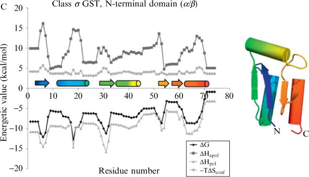
PCA was performed on of 120 human proteins, comprising more than 17,000 residues. Briefly, the ΔG, ΔHapol, Δ, and TΔSconf were computed as a function of residue for each protein using the COREX algorithm as described previously. These four-dimensional data were centered and the eigenvectors and eigenvalues (Table 11.1) were computed from the covariance matrix using standard methods (Manly, 1986; Press et al., 1992; Vertrees, 2008).
Table 11.1.
Eigenvectors (principal components, PC) and eigenvalues (variances) of four-dimensional energetic profile space
| Eigenvector | ΔG | ΔHapol | ΔHpol | TΔSconf | Eigen value | Fractional Variance |
|---|---|---|---|---|---|---|
| PC1 | −0.55 | 0.65 | −0.51 | −0.09 | 24.07 | 0.752 |
| PC2 | 0.15 | 0.69 | 0.70 | 0.11 | 7.04 | 0.220 |
| PC3 | 0.59 | 0.22 | −0.23 | −0.74 | 0.85 | 0.027 |
| PC4 | −0.57 | −0.23 | 0.44 | −0.66 | 0.02 | 0.001 |
| Average Energeticsa | −8.14 | 9.53 | −11.72 | −4.56 |
In units of kcal/mol, at simulated temperature and pH of 25.°C and 7.0, respectively.
Of note is that the first three principal components captured 99.2% of the total variance in the dataset (Fig. 11.2). There was a sharp decrease in the magnitude of the eigenvalues indicating a nonrandom signal and supporting the use of principal components analysis in this application. Notably, principal component 1 (PC1) explained more than 75% of the variance. Interpretation of the eigenvectors as a rotation matrix indicated the linear combination of energetic terms that defined the principal axes (Table 11.1). These results provided a biophysical understanding of the energetic profile space of proteins (J. Vertrees, J. O. Wrabl, and V. J. Hilser, manuscript in preparation).
Figure 11.2.
Variance of four-dimensional energetic profile space explained by principal components. Percentage variance of each principal component (i.e., eigenvalue in Table 11.1) is displayed. Clearly the first principal component accounts for the majority of variance and the first two components account for almost all variance. Therefore, subsequent energetic profiles may be greatly simplified by using only the first component instead of the four thermodynamic quantities ΔG, ΔHapol, ΔHpol, and TΔSconf.
5. Energetic Profiles are Conserved Between Homologous Proteins
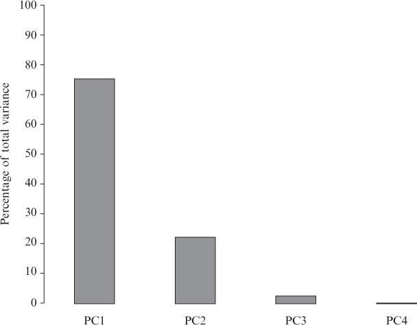
As Fig. 11.2 suggests, the first three principal components provide a set of noncorrelated descriptors from which to generate energetic profiles of proteins. Fig. 11.3 shows the proteins described in Fig. 11.1, with their redefined energetic profiles resulting from centering and rotating according to the eigenvectors in Table 11.1. It is important to note that PCA orders the resulting eigenvectors by the magnitudes of their corresponding eigenvalues in a decreasing manner. Therefore, the amount of variance explained by the first principal component is greatest, the amount explained by the second next greatest, and so forth. This is seen in Figs. 11.3A–C in the following way: once the data are projected onto the principal components, the projected data points have the largest range (or highest variance) directly incident to the first principal component. Consequently, the PC1 curves in Figs. 11.3A–C always have larger ranges than either PC2 or PC3, a reflection of the fact that PC1 contains the most information of the three. Interestingly, stability and the apolar and polar enthalpies contributed approximately equally to PC1.
Figure 11.3.
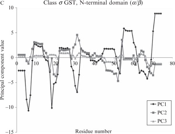
Principal components transformed energetic profiles of three diverse protein structures. Energetic profiles of the structures of Fig. 11.1 are displayed as three transformed datasets, derived from the four thermodynamic quantities in Fig. 11.1 and transformed by the first three eigenvectors of Table 11.1.
Could energetic profiles, though apparently transcendent of the secondary and tertiary structural details of proteins, illuminate our understanding of the physical principles of protein structure and evolution? Comparison of two or more energetic profiles was necessary to address this question. Two identical structures are expected to result in identical energetic profiles, given the nature of the COREX algorithm. This result, though perhaps predictable for highly structurally similar proteins without insertions or deletions, was not obvious in general due to the difficulty of optimally aligning multidimensional energetic profiles of varying length. At least two approaches for aligning energetic profiles could be envisioned: (1) analyze the proteins and directly align the thermodynamic profiles, or (2) align their sequences or high-resolution structures and investigate the correlated thermodynamics of the equivalenced residues. We have actively pursued both approaches, and they have converged on a common result: energetic profiles are largely conserved between homologous proteins, diagnostic of particular folds, and thus appear to be relevant in protein evolution.
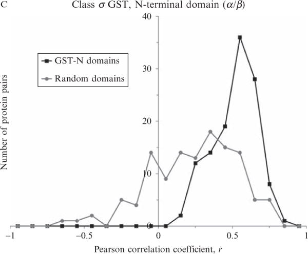
Using the structural alignment approach, conservation of energetic profiles was demonstrated over a large-scale representative sample of fold space, described by Fig. 11.4. Diverse protein domains from the ASTRAL compendium (Chandonia et al., 2004), as classified in the SCOP hierarchy (Murzin et al., 1995), were pairwise structurally aligned and their energetic profiles (from PC1) were equivalenced according to the structural alignment (Fig. 11.4A). Importantly, in this experiment the SCOP classification provided a reasonable assessment of the evolutionary relationship between two proteins: if two proteins belonged to the same SCOP family, they were likely homologous. If they belonged to different SCOP secondary-structure classes, they were likely nonhomologous. A Pearson linear correlation coefficient (Press et al., 1992) was then computed between the two sets of equivalenced energetic values (Fig. 11.4B). These correlations were tabulated for both homologous and nonhomologous pairs exhaustively taken from the ASTRAL representative database, over 1 million pairs total. The probability distributions in Fig. 11.4C clearly demonstrate that homologous proteins have highly correlated energetic profiles, while nonhomologous proteins were less correlated. It is emphasized that the homologous proteins analyzed in Fig. 11.4 were relatively distant evolutionarily, on average exhibiting twilight zone (i.e., <25%) pairwise sequence identity, signifying that energetic comparisons were nontrivial.
Figure 11.4.
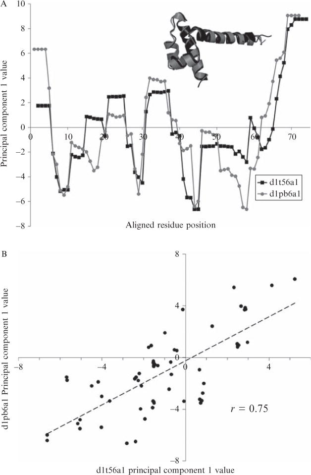
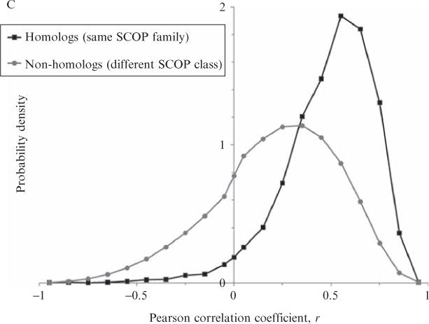
Probability densities of Pearson correlations of energetic profiles between homologous and nonhomologous proteins. 1866 protein domains of 100 residues or less were taken from the ASTRAL 1.69 database of 40% maximum sequence identity representatives (Chandonia et al., 2004); this set constitutes an arguably exhaustive sampling of known fold space. The domains were structurally aligned using DALI (Holm and Park, 2000) in an all-versus-all fashion (Fig. 11.4A, inset; the example shows a homologous engrailed homeodomain pair superimposed with an RMSD of 1.5 Å according to the DALI alignment). Then, energetic profiles were computed for each domain using COREX (run under the parameters listed in the Fig. 11.1 legend) and the first eigenvalue given in Table 11.1 was used to transform each four-dimensional profile into one-dimensional principal component space. First principal components from each member of all possible pairs of proteins were equivalenced according to the DALI structure alignment (Fig. 11.4A) and a Pearson linear correlation coefficient, r, was computed for each pair (Fig. 11.4B). The first and last four residues in each energetic profile, if part of the structural alignment, were ignored in the correlation because of sliding window end effects in the COREX algorithm. To reduce noise in the correlations, only pairs of proteins with resolutions less than 2.5 Å and structure alignments greater than 20 residues were considered. The densities of correlations corresponding to homologous and nonhomologous protein pairs (as defined by belonging to the same SCOP family or different SCOP secondary structure classes, respectively) were normalized such that their total areas equaled 1 (Fig. 11.4C). There were a total of 3715 homologous pairs and 547,600 nonhomologous pairs analyzed. Clearly, homologous protein pairs exhibited similar energetic profiles, as the median correlation between energetic profiles of homologous proteins was approximately r = 0.6, and the median correlation for nonhomologs was approximately r = 0.3.
Does the conservation of energetic profiles extend deeper than just pairs of proteins? This question was addressed by similar experiments using multiple sequence alignments of entire protein families as proxy for pairwise equivalencies of energetic profiles. Results in Fig. 11.5 demonstrate similar results for protein families composed of many aligned sequences: energetic profiles were correlated when the proteins were homologous but were less correlated when the sequences were unrelated.
Figure 11.5.
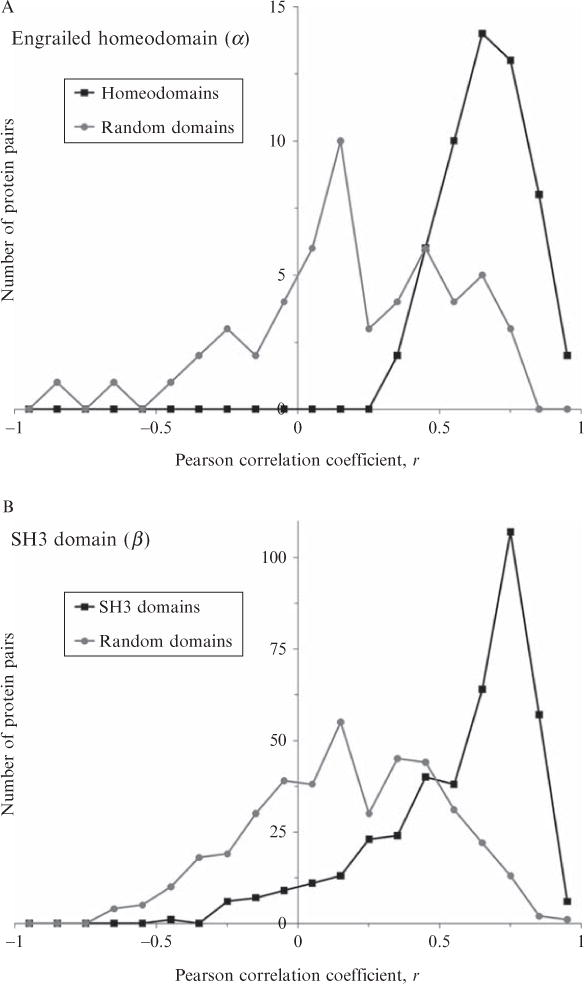
Distributions of Pearson correlations of energetic profiles within three protein-fold families. All domains (≤100 residues) of three SCOP families contained in the ASTRAL 1.69 40% representatives database were extracted: homeodomain (a.4.1.1, 11 members), SH3-domains (b.34.2.1, 29 members), glutathione S-transferase, N-terminal domain (c.47.1.5, 16 members). Each family was subjected to multiple sequence alignment using PROMALS3D (Pei et al., 2008). A randomly chosen set of nonhomologous domains, equal in members and chain lengths, was also multiply aligned as a control for each family. Then, pairwise Pearson correlation coefficients were computed in an all-versus-all fashion for each family and control, as described in the Fig. 11.4 legend. Distributions of these correlations clearly demonstrated that energetic profiles were similar within protein families. Median correlation coefficients for all families were greater than r = 0.6, and median correlations for all unrelated proteins in the control alignments were less than r = 0.3.
Note in both Figs. 11.4C and 11.5 that in some cases even nonhomologous proteins exhibited moderately high correlations while in other cases homologous proteins exhibited moderately low correlations. We have observed at least two artifactual reasons for these observations. First, an unavoidable property of the Pearson correlation coefficient is that high correlations are statistically more likely with fewer numbers of points, as is often the case for alignments of nonhomologous proteins with low sequence or structure similarity. Second, the ASTRAL compendium by design contains examples of clearly homologous proteins that undergo conformational changes across multiple crystal structures. These homologs were not removed during our analyses, and the different structures correctly resulted in different computed energetics, thus weakening specific correlations. However, we believe that a subset of these moderately high correlations between nonhomologs reflect regions of true thermodynamic or structural similarity between ostensibly unrelated proteins, one example of which is described subsequently in this chapter. This result suggests that thermodynamic information, while diagnostic of known evolutionary relationships, could complement existing classifications by uncovering new relationships. This subset of regions of true thermodynamic similarity between unrelated proteins will be the focus of future investigations.
6. Direct Alignment of Energetic Profiles Based on a Variant of the CE Algorithm
A second strategy for comparing two energetic profiles involves treating the profiles as hyperdimensional structures for direct alignment. This is a difficult task because of the large problem space and the inclusion of gaps for two proteins of different lengths. In fact, any practical solution must formally be labeled “near-optimal” because, analogous to structure alignment, this problem is NP complete (Holm and Sander, 1995a; Lathrop, 1994). There exist numerous methods to determine near-optimal subsets of residues to be aligned from two proteins. Some include difference of distance matrices (DALI) (Holm and Sander, 1995b), combinatorial extension (CE) of the optimal path (Shindyalov and Bourne, 1998), genetic algorithms (Szustakowski and Weng, 2000), deterministic annealing (Chen et al., 2005), iterated double dynamic programming (Taylor, 1999), and heuristics combined with dynamic programming (Zhang and Skolnick, 2005). The two most often applied methods are DALI and CE, and we have adapted both methods to allow multidimensional energetic profiles as input. Although a systematic comparison of the utility of each method is beyond the scope of this chapter, CE was generally preferred because, in our hands, it exhibited greater efficiency and produced longer energetic alignments. CE also makes no assumptions about secondary structure (as is the case with the current version of DALI), and we desired alignments based solely on thermodynamic criteria without regard to sequence or three-dimensional structure characteristics.
To modify the CE algorithm for our purposes, we considered the following. CE is based on operations that are performed on two important parameter matrices, the distance matrix and the similarity matrix. Let V be a given vector set with m vectors of dimension n. These vectors might be (x, y, z) structure coordinates; in such a case n would equal 3 and m would equal the number of residues observed in the crystal structure. In contrast, these vectors could be energetic profiles where n equals 4 principal components and m equals the number of residues in the protein. In either case, a distance matrix for the vector set V is the matrix D such that each element of di,j of D represents the Euclidean distance from vector vi to vector vj. Symbolically,
| (11.13) |
In Eq. (11.13), indices i and j cover all possible pairs of residues in the protein. Because the distance from point vi to point vj is identical to the distance from vj to vi, distance matrices are symmetric.
Next, let a and b be two vector sets, with m and p entries of dimension n, respectively. Furthermore, let A and B be their respective distance matrices of sizes m ×m and p × p, respectively, created from Eq. (11.13). The similarity matrix, S, is defined as:
| (11.14) |
where w is a fixed window size. In the original CE algorithm w = 8 residues, and in our work w is usually less than 30.
The similarity matrix therefore measures the similarity between two coordinate or energetic substructures, one from vector set a anchored at residue i to i + k and the other from vector set b anchored at j to j + k. High values denote dissimilar regions, low values denote similar regions, and zero is an exact match. Because the distance from points (ai, aj) in distance matrix A is not necessarily the same as the distance from points (bi, bj) in distance matrix B, not all similarity matrices are symmetric. In fact, they are only symmetric when A is equivalent to B. Good scoring sets of contiguous residues, or paths, can be quickly read off a similarity matrix. For example, to find the best path through the similarity matrix, one starts in the lower left corner and traces to the upper right corner along the lowest scoring diagonal path. Every (i, j) element in the similarity matrix deemed a “good” match according to a user-defined score threshold then pairs together residue i in protein A to residue j in protein B. Gaps are naturally allowed: move one or more positions to the up or right in the similarity matrix. Thus, two protein structures, or energetic profiles of any number of dimensions, may be optimally aligned from their similarity matrix.
7. CE Algorithm Described for Structure Coordinates
CE finds the longest path of lowest score through the similarity matrix for two given protein structures. It can start anywhere in the similarity matrix (although S1,1 is a good choice as it ensures consideration of the longest possible path first) and compares that starting entry, for example Si,j, with a predefined cutoff measure of 3.0 Å. If Si,j > 3.0 Å, then the substructures anchored at i and j in proteins A and B, respectively, are not a good match and are thus ignored. If this is the case, Si+1,j is considered. Once i is exhausted, or the path has gapped 30 times, i is reset and j is incremented. If Si,j 3.0 Å then that residue pair (i, j) is stored and (i + w, j + w) (i.e., (i + 8, j + 8)), is considered. The algorithm is repeated until the similarity matrix is exhaustively searched (using their heuristics to prune spurious low-scoring paths). At this point, the result is the longest possible, best scoring subsets of residues from the two structures. One can then move on to the next step of optimal rigid-body alignment. This variant of CE has been made available to the community on the PyMOL Wiki site (http://www.pymolwiki.org/index.php/Cealign).
CE uses knowledge of protein structures to introduce a few heuristics to decrease the running time. First, CE partitions the protein sequence into windows of eight residues; this decreases the number of combinations to inspect. Second, CE ignores the distances between a residue and its two sequence neighbors because this distance varies little between residues. For example, the distance between an alpha carbon and its sequence neighbor’s alpha carbon is, with high probability, 3.8 Å; any deviation is biophysically unlikely or of insufficient magnitude to impact the calculation and is thus ignored.
8. Necessary Deviations from the CE Algorithm to Accommodate Energetic Profiles
Not surprisingly, numerical values of energetic profiles do not conform to assumptions made in the CE algorithm regarding the numerical values of protein structure coordinates. This necessitated investigation of every structure-based assumption in CE; the assumptions and necessary changes are enumerated here. First, because sequence neighbors may have large discontinuities in energetic space, during the equivalence step a modified algorithm must consider neighbor-neighbor distances while the original CE algorithm did not. Second, also because of extremely large dynamic range of values, some normalization of the energetic data was necessary. Without normalization, large numerical jumps (e.g., 15 energetic units versus 3.0 Å in Cartesian coordinates) would dominate the similarity measures and cause spurious matches. Our variant of CE was built such that during construction of the similarity matrix, the distance matrices were locally scaled such that the largest distance in each submatrix is 1.0. This modification enabled window-based structure scaling. Though it increased the running time of the algorithm, it allowed the algorithm to be more tolerant of the vagaries of scale and produced more accurate energetic profile alignments. A third deviation from the original CE algorithm occurred during the refinement step. CE called for a sequence-based refinement step. The variant algorithm removed the refinement step as alignments based solely on energetic information were desired. Finally, the last set of deviations dealt with the empirically defined parameters enforced by CE. The original algorithm required a window size (eight residues was determined to be optimal), a maximum gap of 30 residues, a minimum cutoff of 3.0 Å, and a minimum path cutoff of 4.0 Å. These values were determined from fine tuning CE against known structure databases. Unfortunately, we did not have the luxury of known thermodynamic homology—indeed that was the question we wished to address. We estimated these tunable parameters by comparison of three known structure families and clustering the results (data not shown). The optimal distance cutoffs chosen were 0.040w, where w was the window size in residues. Both cutoffs were set to this value in the energetic comparisons described subsequently. The longest continuous energetic substructures were found by setting the maximum gap to 0, with iterative increases of the window size from 6 to 26. This empirical procedure allowed initial detection of smaller as well as larger regions of energetic similarity.
In protein structure comparison, the root-mean-square deviation (RMSD) of the equivalenced atoms is often used when checking the quality of the alignment. RMSD provides a quantitative measure of how good the alignment is but does not consider either the number of gaps or the length of the alignment. Thus, RMSD alone can be a misleading measure of quality; for example, an alignment with 200 equivalenced atoms and a 1.4 Å RMSD with no internal gaps would be expected to be more biologically relevant than a gapped alignment exhibiting the same RMSD over only 20 atoms. Therefore, in scoring the quality of energetic profile alignments we employed the CE score, which has been demonstrated to better represent alignment quality (Jia et al., 2004). The CE score is defined as,
| (11.15) |
In Eq. (11.15), RMSD is the minimum RMSD (Kabsch, 1976, 1978) of the energetic profile-equivalenced CA atoms, L is the number of equivalenced residues, and G is the number of internal gaps in the energetic profile alignment. An implementation of the Kabsch minimum RMSD algorithm used in this work has been made freely available to the community on the PyMOLWiki site (http://www.pymolwiki.org/index.php/Kabsch).
9. Towards a Thermodynamic Homology of Fold Space: Clustering Energetic Profiles using STEPH
Given energetic profiles of proteins and a method to compare them, we could now consider the organization of thermodynamic fold space. Which proteins were related and why? What families of folds could be identified using only thermodynamic information? Answering such questions may provide a novel viewpoint to understand the evolution of proteins. We employed our CE variant in an all-against-all fashion versus a subset of a thermodynamic database of 120 proteins previously studied in our laboratory (Larson and Hilser, 2004). We then analyzed these results using agglomerative hierarchical clustering tools to determine apparent thermodynamic relationships. Finally, we compared thermodynamic relationships with standard structure-based relationships.
Our CE variant, Structural Thermodynamic Ensemble-based Protein Homology (STEPH) compared each energetic profile to every other, providing a dissimilarity matrix of CE scores where each protein was represented as a point in a high-dimensional energetic fold space. We next desired to divide the space into mutually exclusive regions and thereby define thermodynamic fold families. We started with the straightforward clustering method of Ward (1963), as implemented in the R language (http://www.r-project.org), to cluster the dissimilarity matrix. As mentioned earlier, we chose to restrict the gap parameter to zero in STEPH, otherwise highly fragmented alignments are observed. To find longer alignments, we iterated over a window size of 6 to 26 residues, retaining optimal energetic alignments. Each iteration’s results were turned into a distance matrix for that window size. Subsequently, each distance matrix was averaged into a global distance matrix and the global matrix was clustered.
In detail, for each window size, the following binary mask M was applied to the alignment score matrix:
| (11.16) |
Therefore, if the energetic profile of a protein was close to another (i.e., within the 25th quantile), then its distance was reset to 0. If the profile was not close, its distance was reset to 1. In other words, for each window size, specific relationship information was retained and noise was disregarded, as defined by the 25th quantile. The 25th quantile was empirically chosen to retain some longer distances, as the 5th quantile, for example, retained too few profiles and was not a useful cutoff. The binary-masked matrices were added to form an averaged matrix for distance representation, and this averaged matrix was clustered using Ward’s algorithm as implemented by the hclust function in R.
This procedure was applied to five small families of homologous proteins. The procedure was run on both structure coordinates as well as energetic profiles. Results are displayed in Fig. 11.6 as phylogenetic trees, although presently we interpret these trees simply as clusters and do not necessarily consider branch lengths as evolutionarily meaningful.
Figure 11.6.
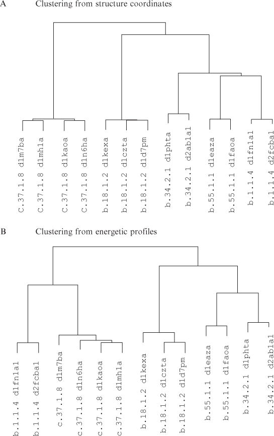
Cluster trees built from either structure coordinates or energetic profiles of five homologous protein-fold families. Protein domains were contained in our previously studied human protein thermodynamic database (Larson and Hilser, 2004). SCOP families represented are G proteins (c.37.1.8), discoidin (b.18.1.2), SH3 domains (b.34.2.1), Pleckstrin-homology domains (b.55.1.1), and I set domains (b.1.1.4). Trees were built using agglomerative hierarchical clustering, as described in text, with input data from CE structure alignments or STEPH, our variant of CE, energetic profile alignments. (A) Clustering from three-dimensional structure coordinates. SCOP families are clearly segregated with all-beta proteins on a separate branch from the alpha/beta proteins. (B) Clustering from three-dimensional energetic profiles. SCOP families are again properly segregated but the I set domains have moved to the alpha/beta branch, for thermodynamic reasons described in the text.
The major difference between the arrangement of the structure-based clustering and the energetic profile-based clustering is the location of the 1fnlA/2fcbA branch. In structural terms it has been determined to have some propinquity with the folds on the right side of the tree (Fig. 11.6A). The results from the clustering show the branch moving to the opposite side of the tree (Fig. 11.6B). What is the origin of this observation? To answer this, we consider the following. First, inspection of the optimal alignments and scores showed that the 1fnlA/2fcbA branch scored well thermodynamically with respect to the 1m7bA branch. Fig. 11.7 indicates why; the overlapping segments are comprised of residues 115–168 in 1fnlA and 39– 92 in 1m7bA. In Figs. 11.7A–D the two regions are aligned according to the STEPH alignment and their residues renumbered from 1 to more easily discuss the overlapping features. Though the overlap in general appears acceptable, we focus on two regions: spanning residues 10–18 and 35–42.
Figure 11.7.
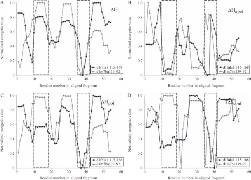
Energetic profiles of two fragments of STEPH aligned nonhomologous proteins. A subset of 54 residues from the complete energetic alignment is shown: residues 115–168 (PDB numbering) of d1fnla1 and residues 39-92 (PDB numbering) of d1m7ba1. The aligned subset has been renumbered starting from 1. For clarity, the principal components transformed profiles are displayed as the original four energetic quantities: (A) local stability (ΔG), (B) apolar solvation enthalpy (ΔHapol), (C) polar solvation enthalpy (ΔHpol), and D. conformational entropy (TΔSconf). Energetic profiles are normalized so that minimum values within each protein equal 0 and maximum values equal 1. Regions 10–18 and 35–42, discussed in text, are boxed in each panel.
The first region shows high overlap on the apolar enthalpy dimension with some variation on the polar enthalpy dimension. Inspection of the structural fragments is revealing (Fig. 11.8). The region from 1m7bA consists mainly of apolar residues in a loop fully exposed to solvent. Thus, upon unfolding of this region, the energetic contribution will be a relatively low amount of polar surface area with a relatively low amount of apolar complementary surface area being exposed as well. This effectively balances the apolar to polar enthalpy ratio: low direct polar exposure, low complementary apolar exposure. Thus, the apolar enthalpy dimensions for the two proteins should be relatively similar throughout this region, thus the overlap of apolar enthalpy. This also explains why the conformational entropy values for this region are vastly different, considering their locations in secondary and tertiary structure.
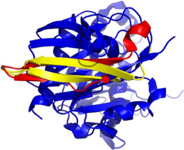
Figure 11.8.

Molecular rationalization of STEPH aligned fragments of nonhomologous proteins. Fragments of d1fnla (PDB 1fnlA residues 115–168) and d1m7ba1 (PDB 1m7bA residues 39–92) as energetically aligned by STEPH are displayed in green and light blue, respectively. Renumbered residues 10–18 of the 1m7bA aligned fragment discussed in the text are displayed in yellow, with apolar solvent exposed side chains explicitly shown.
The second region of importance spans residues 35–42. This region in both proteins exhibits similar values for all four descriptors, resulting in a good alignment. Thus, exploring these two subsequences shows that proteins have at their disposal various combinations of mechanisms to modulate local stability, enthalpy and entropy values. As reinforced by the energetic profiles shown in Fig. 11.1, the various mechanisms are simply not apparent in the tenets of “helices and sheets are stable while loops are unstable”.
10. Energetic Profiles Provide a Vehicle to Discover Conserved Substructures in the Absence of Known Homology
Not infrequently, substantial structural overlap was observed between two proteins with no known homology. This phenomenon occurs in the 1fnl and 1m7b proteins contained in the example of Fig. 11.6. They exhibited structural overlap of 24 residues, determined from their energetic profiles alone. Fig. 11.9 shows the two proteins with their thermodynamically aligned segments highlighted. Notice when structurally superimposed, these segments also aligned well (3.1 Å RMSD). We believe this phenomenon is characteristic in general of fold space, as exemplified by the presence of moderately high energetic correlations between nonhomologous proteins mentioned above (Fig. 11.4C).
Figure 11.9.
Structurally similar regions of two nonhomologous proteins revealed by alignment of energetic profiles. Two structurally similar regions of 24 residues each, determined to be energetically similar from STEPH alignment as discussed in the text, are highlighted in red (d1fnla1) and yellow (d1m7ba). The remainders of both proteins are displayed in blue.
A second observation from these two overlapping substructures is that they were centered upon loops or coils. This hinted at an underlying principle of energetic profile alignments being anchored at loops or coils with different intervening secondary structure elements. In other words, if the loops/coils aligned well, then the intervening secondary structure elements aligned because of shared topological features affecting the local energetics, instead of shared secondary structure type. Because loops and coils are typically highly solvent accessible in globular proteins, perhaps it is not surprising that they exhibit thermodynamically uniform characteristics, in contrast to helices and strands which may have varying degrees of solvent exposure.
11. Conclusion
Energetic profiles, derived from an experimentally validated statistical mechanical representation of a protein’s native state ensemble, are demonstrated to be a novel diagnostic of diverse protein folds. Consequently, new tools, such as the STEPH algorithm described in this work, are necessary to compute, compare, and classify energetic profiles. Initial analysis of a large representative sample of protein-fold space suggests that energetic profiles are evolutionarily relevant. However, the information in energetic profiles, although mostly complementary to the sequence, structure and functional descriptors used in current databases, also has the potential to reclassify protein-fold space. We believe the integration of this thermodynamic information into existing classification schemes will increase understanding of the physical principles of protein structure and the mechanisms of protein evolution.
Acknowledgments
Supported by NIH grant (GM63747), NSF grant (MCB0406050), and the Robert A. Welch Foundation (H-1461).
References
- Alva V, Koretke KK, Coles M, Lupas AN. Cradle-loop barrels and the concept of metafolds in protein classification by natural descent. Curr Opin Struct Biol. 2008;18:358–365. doi: 10.1016/j.sbi.2008.02.006. [DOI] [PubMed] [Google Scholar]
- Babu CR, Hilser VJ, Wand AJ. Direct access to the cooperative substructure of proteins and the protein ensemble via cold denaturation. Nat Struct Mol Biol. 2004;11:352–357. doi: 10.1038/nsmb739. [DOI] [PubMed] [Google Scholar]
- Chandonia JM, Hon G, Walker NS, Lo Conte L, Koehl P, Levitt M, Brenner SE. The ASTRAL compendium in 2004. Nucleic Acids Res. 2004;32:D189–D192. doi: 10.1093/nar/gkh034. [DOI] [PMC free article] [PubMed] [Google Scholar]
- Chen L, Zhou T, Tang Y. Protein structure alignment by deterministic annealing. Bioinformatics. 2005;21:51–62. doi: 10.1093/bioinformatics/bth467. [DOI] [PubMed] [Google Scholar]
- Day R, Beck DA, Armen RS, Daggett V. A consensus view of fold space: Combining SCOP, CATH, and the Dali Domain Dictionary. Protein Sci. 2003;12:2150–2160. doi: 10.1110/ps.0306803. [DOI] [PMC free article] [PubMed] [Google Scholar]
- Dunbrack RL., Jr Sequence comparison and protein structure prediction. Curr Opin Struct Biol. 2006;16:374–384. doi: 10.1016/j.sbi.2006.05.006. [DOI] [PubMed] [Google Scholar]
- Ferreon JC, Volk DE, Luxon BA, Gorenstein DG, Hilser VJ. Solution structure, dynamics, and thermodynamics of the native state ensemble of the Sem-5 C-terminal SH3 domain. Biochemistry. 2003;42:5582–5591. doi: 10.1021/bi030005j. [DOI] [PubMed] [Google Scholar]
- Finn RD, Tate J, Mistry J, Coggill PC, Sammut SJ, Hotz HR, Ceric G, Forslund K, Eddy SR, Sonnhammer EL, Bateman A. The Pfam protein families database. Nucleic Acids Res. 2008;36:D281–D288. doi: 10.1093/nar/gkm960. [DOI] [PMC free article] [PubMed] [Google Scholar]
- Greene LH, Lewis TE, Addou S, Cuff A, Dallman T, Dibley M, Redfern O, Pearl F, Nambudiry Rekha, Reid A, Sillitoe I, Yeats C, et al. The CATH domain structure database: New protocols and classification levels give a more comprehensive resource for exploring evolution. Nucleic Acids Res. 2007;35:D291–D297. doi: 10.1093/nar/gkl959. [DOI] [PMC free article] [PubMed] [Google Scholar]
- Gu J, Hilser VJ. Predicting the energetics of conformational fluctuations in proteins from sequence: A strategy for profiling the proteome. Structure. 2008;16:1627–1637. doi: 10.1016/j.str.2008.08.016. [DOI] [PMC free article] [PubMed] [Google Scholar]
- Heger A, Mallick S, Wilton C, Holm L. The global trace graph, a novel paradigm for searching protein sequence databases. Bioinformatics. 2007;23:2361–2367. doi: 10.1093/bioinformatics/btm358. [DOI] [PubMed] [Google Scholar]
- Henzler-Wildman K, Kern D. Dynamic personalities of proteins. Nature. 2007;450:964–972. doi: 10.1038/nature06522. [DOI] [PubMed] [Google Scholar]
- Hilser VJ. Modeling the native state ensemble. Methods Mol Biol. 2001;168:93–116. doi: 10.1385/1-59259-193-0:093. [DOI] [PubMed] [Google Scholar]
- Hilser VJ, Freire E. Structure-based calculation of the equilibrium folding pathway of proteins. Correlation with hydrogen exchange protection factors. J Mol Biol. 1996;262:756–772. doi: 10.1006/jmbi.1996.0550. [DOI] [PubMed] [Google Scholar]
- Hilser VJ, Garcia-Moreno EB, Oas TG, Kapp G, Whitten ST. A statistical thermodynamic model of the protein ensemble. Chem Rev. 2006;106:1545–1558. doi: 10.1021/cr040423+. [DOI] [PubMed] [Google Scholar]
- Holm L, Sander C. 3-D lookup: Fast protein structure database searches at90% reliability. Proc Int Conf Intell Syst Mol Biol. 1995a;3:179–187. [PubMed] [Google Scholar]
- Holm L, Sander C. Protein structure comparison by alignment of distance matrices. J Mol Biol. 1995b;233:123–138. doi: 10.1006/jmbi.1993.1489. [DOI] [PubMed] [Google Scholar]
- Igumenova TI, Frederick KK, Wand AJ. Characterization of the fast dynamics of protein amino acid side chains using NMR relaxation in solution. Chem Rev. 2006;106:1672–1699. doi: 10.1021/cr040422h. [DOI] [PMC free article] [PubMed] [Google Scholar]
- Jia Y, Dewey TG, Shindyalov IN, Bourne PE. A new scoring function and associated statistical significance for structure alignment by CE. J Comp Biol. 2004;11:787–799. doi: 10.1089/cmb.2004.11.787. [DOI] [PubMed] [Google Scholar]
- Kabsch W. A solution for the best rotation to relate two vector sets. Acta Cryst Sec A. 1976;32:922–923. [Google Scholar]
- Kabsch W. A discussion of the solution for the best rotation to relate two vector sets. Acta Cryst Sec A. 1978;34A:827–828. [Google Scholar]
- Kinch LN, Grishin NV. Evolution of protein structures and functions. Curr Opin Struct Biol. 2002;12:400–408. doi: 10.1016/s0959-440x(02)00338-x. [DOI] [PubMed] [Google Scholar]
- Kolodny R, Petrey D, Honig B. Protein structure comparison: Implications for the nature of fold space, and structure and function prediction. Curr Opin Struct Biol. 2006;16:393–398. doi: 10.1016/j.sbi.2006.04.007. [DOI] [PubMed] [Google Scholar]
- Kriventseva EV, Fleischmann W, Zdobnov EM, Apweiler R. CluSTr: A database of clusters of SWISS-PROT+TrEMBL proteins. Nucleic Acids Res. 2001;29:33–36. doi: 10.1093/nar/29.1.33. [DOI] [PMC free article] [PubMed] [Google Scholar]
- Larson SA, Hilser VJ. Analysis of the “thermodynamic information content” of a Homo sapiens structural database reveals hierarchical thermodynamic organization. Protein Sci. 2004;13:1787–1801. doi: 10.1110/ps.04706204. [DOI] [PMC free article] [PubMed] [Google Scholar]
- Lathrop RH. The protein threading problem with sequence amino acid interaction preferences is NP complete. Protein Eng. 1994;7:1059–1068. doi: 10.1093/protein/7.9.1059. [DOI] [PubMed] [Google Scholar]
- Lecomte JT, Vuletich DA, Lesk AM. Structural divergence and distant relationships in proteins: Evolution of the globins. Curr Opin Struct Biol. 2005;15:290–301. doi: 10.1016/j.sbi.2005.05.008. [DOI] [PubMed] [Google Scholar]
- Liu T, Whitten ST, Hilser VJ. Functional residues serve a dominant role in mediating the cooperativity of the protein ensemble. Proc Natl Acad Sci USA. 2007;104:4347–4352. doi: 10.1073/pnas.0607132104. [DOI] [PMC free article] [PubMed] [Google Scholar]
- Manly BFJ. Multivariate statistical methods: A primer. Chapman and Hall; New York: 1986. [Google Scholar]
- Milne JS, Xu Y, Mayne LC, Englander SW. Experimental study of the protein folding landscape: Unfolding reactions in cytochrome c. J Mol Biol. 1999;290:811–822. doi: 10.1006/jmbi.1999.2924. [DOI] [PubMed] [Google Scholar]
- Mittermaier A, Kay LE. New tools provide new insights in NMR studies of protein dynamics. Science. 2006;312:224–228. doi: 10.1126/science.1124964. [DOI] [PubMed] [Google Scholar]
- Murzin AG, Brenner SE, Hubbard T, Chothia C. SCOP: A structural classification of proteins database for the investigation of sequences and structures. J Mol Biol. 1995;247:536–540. doi: 10.1006/jmbi.1995.0159. [DOI] [PubMed] [Google Scholar]
- Orban J, Alexander P, Bryan P, Khare D. Assessment of stability differences in the protein G. B1 and B2 domains from hydrogen-deuterium exchange: Comparison with calorimetric data. Biochemistry. 1995;34:15291–15300. doi: 10.1021/bi00046a038. [DOI] [PubMed] [Google Scholar]
- Pan H, Lee JC, Hilser VJ. Binding sites in Escherichia coli dihydrofolate reductase communicate by modulating the conformational ensemble. Proc Natl Acad Sci USA. 2000;97:12020–12025. doi: 10.1073/pnas.220240297. [DOI] [PMC free article] [PubMed] [Google Scholar]
- Press WH, Teukolsky SA, Vetterling WT, Flannery BP. Numerical recipes in C: The art of scientific computing. Cambridge University Press; New York: 1992. [Google Scholar]
- Russell RB. Classification of protein folds. Mol Biotechnol. 2002;20:17–28. doi: 10.1385/MB:20:1:017. [DOI] [PubMed] [Google Scholar]
- Shindyalov IN, Bourne PE. Protein structure alignment by incremental combinatorial extension (CE) of the optimal path. Protein Eng. 1998;11:739–747. doi: 10.1093/protein/11.9.739. [DOI] [PubMed] [Google Scholar]
- Shindyalov IN, Bourne PE. An alternative view of protein fold space. Proteins. 2000;38:247–260. [PubMed] [Google Scholar]
- Szustakowski JD, Weng Z. Protein structure alignment using a genetic algorithm. Proteins Struct Funct Genet. 2000;38:428–440. doi: 10.1002/(sici)1097-0134(20000301)38:4<428::aid-prot8>3.0.co;2-n. [DOI] [PubMed] [Google Scholar]
- Tatusov RL, Fedorova ND, Jackson JD, Jacobs AR, Kiryutin B, Koonin EV, Krylov DM, Mazumder R, Mekhedov SL, Nikolskaya AN, Rao BS, Smirnov S, et al. The COG database: An updated version includes eukaryotes. BMC Bioinformatics. 2003;4:41. doi: 10.1186/1471-2105-4-41. [DOI] [PMC free article] [PubMed] [Google Scholar]
- Taylor WR. Protein structure comparison using iterated double dynamic programming. Protein Science. 1999;8:654–665. doi: 10.1110/ps.8.3.654. [DOI] [PMC free article] [PubMed] [Google Scholar]
- Taylor WR. Evolutionary transitions in protein fold space. Curr Opin Struct Biol. 2007;17:354–361. doi: 10.1016/j.sbi.2007.06.002. [DOI] [PubMed] [Google Scholar]
- Vertrees J. A thermodynamic definition of protein folds. Department of Biochemistry and Molecular Biology, Vol. Doctor of Philosophy. University of Texas Medical Branch; Galveston: 2008. p. 159. [Google Scholar]
- Vertrees J, Barritt P, Whitten S, Hilser VJ. COREX/BEST server: A web browser-based program that calculates regional stability variations within protein structures. Bioinformatics. 2005;21:3318–3319. doi: 10.1093/bioinformatics/bti520. [DOI] [PubMed] [Google Scholar]
- Wang S, Gu J, Larson SA, Whitten ST, Hilser VJ. Denatured-state energy landscapes of a protein structural database reveal the energetic determinants of a framework model for folding. J Mol Biol. 2008;381:1184–1201. doi: 10.1016/j.jmb.2008.06.046. [DOI] [PMC free article] [PubMed] [Google Scholar]
- Ward JH. Hierarchical grouping to optimize an objective function. J Am Stat Assoc. 1963;58:236–244. [Google Scholar]
- Whitten ST, Garcia-Moreno BE, Hilser VJ. Ligand effects on the protein ensemble: Unifying the descriptions of ligand binding, local conformational fluctuations, and protein stability. Methods Cell Biol. 2008;84:871–891. doi: 10.1016/S0091-679X(07)84027-1. [DOI] [PubMed] [Google Scholar]
- Whitten ST, Garcia-Moreno EB, Hilser VJ. Local conformational fluctuations can. modulate the coupling between proton binding and global structural transitions in proteins. Proc Natl Acad Sci USA. 2005;102:4282–4287. doi: 10.1073/pnas.0407499102. [DOI] [PMC free article] [PubMed] [Google Scholar]
- Whitten ST, Kurtz AJ, Pometun MS, Wand AJ, Hilser VJ. Revealing the nature of the native state ensemble through cold denaturation. Biochemistry. 2006;45:10163–10174. doi: 10.1021/bi060855+. [DOI] [PubMed] [Google Scholar]
- Wrabl JO, Larson SA, Hilser VJ. Thermodynamic propensities of amino acids in the native state ensemble: Implications for fold recognition. Protein Sci. 2001;10:1032–1045. doi: 10.1110/ps.01601. [DOI] [PMC free article] [PubMed] [Google Scholar]
- Wrabl JO, Larson SA, Hilser VJ. Thermodynamic environments in proteins: Fundamental determinants of fold specificity. Protein Sci. 2002;11:1945–1957. doi: 10.1110/ps.0203202. [DOI] [PMC free article] [PubMed] [Google Scholar]
- Zhang Y, Skolnick J. TM-align: A protein structure alignment algorithm based on the TM-score. Nucleic Acids Res. 2005;33:2302–2309. doi: 10.1093/nar/gki524. [DOI] [PMC free article] [PubMed] [Google Scholar]