Empirical estimation of intravoxel structure with persistent angular structure and Q-ball models of diffusion weighted MRI

Abstract.

The diffusion tensor model is nonspecific in regions where micrometer structural patterns are inconsistent at the millimeter scale (i.e., brain regions with pathways that cross, bend, branch, fan, etc.). Numerous models have been proposed to represent crossing fibers and complex intravoxel structure from in vivo diffusion weighted magnetic resonance imaging (e.g., high angular resolution diffusion imaging—HARDI). Here, we present an empirical comparison of two HARDI approaches—persistent angular structure MRI (PAS-MRI) and Q-ball—using a newly acquired reproducibility dataset. Briefly, a single subject was scanned 11 times with 96 diffusion weighted directions and 10 reference volumes for each of two $b$ values (1000 and $3000\mathrm{s}/{\mathrm{mm}}^2$ for a total of 2144 volumes). Empirical reproducibility of intravoxel fiber fractions (number/strength of peaks), angular orientation, and fractional anisotropy was compared with metrics from a traditional tensor analysis approach, focusing on $b$ values of 1000 and $3000\mathrm{s}/{\mathrm{mm}}^2$. PAS-MRI is shown to be more reproducible than Q-ball and offers advantages at low $b$ values. However, there are substantial and biologically meaningful differences between the intravoxel structures estimated both in terms of analysis method as well as by $b$ value. The two methods suggest a fundamentally different microarchitecture of the human brain; therefore, it is premature to perform meta-analysis or combine results across HARDI studies using a different analysis model or acquisition sequences.

1. Introduction

Diffusion weighted magnetic resonance imaging (MRI) enables noninvasive millimetric mapping of local tissue orientation via sensitivity to directional diffusion on the micrometer scale. The tensor model in diffusion tensor imaging (DTI) has been wildly successful for interpreting this signal in cerebral white matter tracts and reconstructing major fiber pathways in the brain as it is sensitive to fiber orientations.¹ To address DTI’s shortcomings in regions of complex intravoxel structure, high angular resolution diffusion imaging (HARDI) methods acquire and analyze additional data to estimate multiple fiber population orientations per voxel. These methods reveal more elaborate information about the intravoxel structure, e.g., diffusion orientation transform,² spherical deconvolution (SD),^3,4 persistent angular structure (PAS-MRI),⁵ or Q-ball.⁶

Previous large-scale reproducibility studies with DTI have been essential for understanding the empirical behavior of the tensor estimator (e.g., Ref. 7). We perform an in-depth comparison of PAS-MRI and Q-ball as representative variants of HARDI methods. PAS-MRI models the intravoxel diffusion using a discrete number of fiber compartments,⁸ while Q-ball estimates an orientation distribution function (ODF), which is assumed to reflect the underlying fiber orientation distribution through its impact on diffusivity.⁹ PAS has been shown to be more consistent than Q-ball on synthetic data at lower or clinical $b$ values of about $1200\mathrm{s}/{\mathrm{mm}}^2$.^8,10 Meanwhile, Q-ball is effective at higher $b$ values ($\sim 3000\mathrm{s}/{\mathrm{mm}}^2$ or greater).⁶ Previous work on Q-ball has also shown that it resolves multiple fiber orientations for fractional anisotropy (FA) regions $<0.4$.¹¹ While a minimum angle of fiber orientations has not been established for PAS yet, Q-ball has been known to resolve angles down to 45 deg with diminishing accuracy depending on adequate signal-to-noise ratio (SNR).¹² Herein, we compare the empirical reproducibility of PAS-MRI and Q-ball focusing on $b$ values of 1000 and $3000\mathrm{s}/{\mathrm{mm}}^2$. We have also compared the models in terms of agreement between PAS and Q-ball.

In Ref. 13, the authors show that PAS can more consistently resolve crossing fiber voxels compared to Q-ball. PAS has also been shown capable of detecting up to two crossing fibers with robustness in the method in the presence of noisy data.¹⁴ In Ref. 15, improvement in probabilistic index of connectivity (PICo) tractography was shown using a Bingham distribution with compelling PAS results compared with Q-ball. A drawback noted was that PAS-MRI showed a spurious perpendicular peak for fanning structures based on bootstrap validation. In Ref. 16, the authors stated that the fiber orientation distribution methods have a high agreement with probabilistic tractography and PAS-MRI specifically having a sparse connectivity matrix. It has been strongly suggested for further validation using more complex biological phantoms techniques.¹⁷

Previously, the bias and variance of PAS and Q-ball methods have been assessed using relatively small datasets.^5,6,8,9 Region of interest (ROI) analysis has shown that Q-ball retains angular information when $b$ value is brought down to the range of 2000 to $2500\mathrm{s}/{\mathrm{mm}}^2$.¹⁸ Average angular resolution of Q-ball has been estimated to be between 15 deg and 30 deg based on analysis presented in Ref. 19. While analyses of bias have been performed using repeated phantom/synthetic data,¹² verification of these results is important with in vivo data. Q-ball can identify crossing fibers, yet it fails in scenarios where there are fanning or splitting of fibers. In Ref. 20, a comparative reproducibility study of tractography between PAS-MRI and Q-ball was performed for specific ROI’s. Both methods were shown to be highly reproducible with PAS-MRI being slightly superior. Phantom studies¹⁷ on Q-ball using tractography have suggested the need for more reliable validation methods. Here, we offer an extensive empirical scan–rescan validation set on a single subject acquired at multiple $b$ values so the diffusion model fitting methods can be studied on a range of acquisition sequences and quantities of data following large-scale validation work done with DTI.⁷

2. Methods

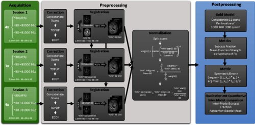
Briefly, the data were preprocessed for each scan session individually and successively registered to the Montreal Neurological Institute (MNI) space template (Fig. 1). Gold standard models were created for each method and $b$ value by concatenating the 11 scans per $b$ value and fitting with each method. Comparisons were performed across repetitions to assess variance/reproducibility, while comparisons among the gold standard scans were performed to assess bias.

Fig. 1.

Flowchart depicting the pipeline of data processing steps.

2.1. DW-MRI Data Measurements

A healthy volunteer was scanned in three different sessions on successive days on a 3T Phillips Scanner with a 32-channel head coil. The first and last scan sessions consisted of four repetitions of 96 gradient directions per $b$ values at each of 1000 and $3000\mathrm{s}/{\mathrm{mm}}^2$. The second session had three repetitions of the protocol. For each $b$-value shell, 10 minimally weighted reference images (b0’s) were also acquired. Voxel resolution for the data is $2.5\mathrm{mm}\times 2.5\mathrm{mm}\times 2.5\mathrm{mm}$ with a matrix of $96\times 96$ and 38 slices. The scan parameters were $\text{multiband}=2$, $\mathrm{SENSE}=2.2$, $\mathrm{TR}=2650\mathrm{ms}$, $\mathrm{TE}=94\mathrm{ms}$, and partial $\mathrm{Fourier}=0.7$. Fold over direction was A-P with a P fat shift. For each set of five shells, an additional diffusion scan was acquired with reverse phase encoded volumes (i.e., fold over direction A-P with A fat shift) with a minimally weighted volume and three diffusion weighting directions with a $b$ value of $1000\mathrm{s}/{\mathrm{mm}}^2$ along the imaging frame cardinal directions, and all other parameters were kept constant. All data were acquired in accordance with the Vanderbilt University Institutional Review Board (IRB) guidelines and with the signed consent of the volunteer.

2.2. Data Preprocessing

Each session was corrected for eddy current motion, patient head movement, and susceptibility distortion with FSL’s topup and eddy.^21,22 Every diffusion weighted shell was preceded by a nondiffusion weighted image (b0) averaged 10 times on the scanner, and each session had four reverse phase encoded b0 volumes. All b0’s including reverse phase encoded b0’s in a session were concatenated and fed as inputs to topup. For eddy all scans in a session were concatenated and then corrected together using the results from topup. Once topup and eddy had been performed, the corrected b0’s from the first session were registered to a 2.5-mm isotropic MNI T2, which was resampled from a 0.5-mm weighted template using six degree of freedom registration.²³ The volumes for the next session were brought to the same space by averaging the b0’s together and registering the combined image to the averaged b0’s in the first session. The same procedure was subsequently done to the last session to bring all three sessions into a common subject-specific pose aligned with MNI space.

Thereafter, all the sessions were normalized by the b0 corresponding to the scan to account for amplitude drift (Fig. 1). A weighted mean b0 was created from all b0 scans in MNI space by a weighted average of all b0’s. The weight was taken as the inverse of the median of all b0 scans in MNI space averaged with the mean of b0’s from all sessions. The final normalization scan was computed by multiplying the weighted mean b0 to the ratio of diffusion weighted scan (in MNI space) to the b0 (in MNI space).

2.3. Data Segmentation

Individual target images (T1 weighted scans) were affine registered to the MNI305 atlas²⁴ and bias corrected with N4²⁵ using advanced normalization tools (ANTs)²⁶ on the atlas and the target images. Nonrigid registration was performed from atlas images to the target image using ANTs and symmetric image normalization algorithm.²⁷ Image and label volumes for the atlas were then deformed to the target space with bicubic and nearest-neighbor interpolation and fused with nonlocal spatial STAPLE^28,29 and Adaboost correction.³⁰ Each individual voxel in the brain was labeled to one of the 133 labels obtained from the multiatlas labeling using the BrainCOLOR protocol.³¹ T1 image labels were brought back to the original target space with the ANTs inverse transformation. All WM labels were concatenated together to create a WM mask. The mask has been used for all reported results with the only exception of the visual glyphs where we have shown all data for the particular slice.

In order to avoid circularity of defining white matter by FA and then examining FA in white matter, we defined the white matter mask based on multiatlas segmentation of the T1-weighted MRI (Figs. 2 and 3). As the histograms show, the structural definition spans the full breadth of white matter configurations [from homogeneous major tracks, to crossing fibers, and even to some regions of partial volume (e.g., very low FA)].

Fig. 2.

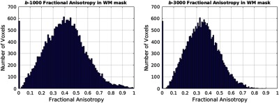
Histogram of FA values in the white mask for both $b$ values of 1000 and $3000\mathrm{s}/{\mathrm{mm}}^2$.

Fig. 3.

Spatial maps of middle axial slice: (a) WM mask, (b) FA in WM mask, and (c) where $\mathrm{FA}<0.3$ in WM mask.

2.4. Q-Ball Reconstruction

Q-ball’s ODF was originally calculated using a funk radon transform⁶ using a sphere in q-space on raw diffusion data. In Ref. 9, the authors showed that a faster and robust Q-ball model can be formed and regularized using spherical harmonics.

The spherical harmonic Q-ball has exhibited different behavior with spherical harmonic orders, which keep even orders to retain symmetry. Previous results have revealed spherical harmonic order shows dependence on the number of gradient directions and $b$ value.³² Additionally, lower order harmonics lead to less angular resolution. High spherical harmonic orders and high $b$ values yield decrease in angular error for high SNR sequences for $b$ values up till $6000\mathrm{s}/{\mathrm{mm}}^2$.⁹ Herein, the parameters chosen were order 8 for the spherical harmonics and the default regularization parameter, which is 0.006. Camino was used for the implementation.³³

2.5. RE-PASMRI Reconstruction

PAS is a special case of SD. The radius of sphere defined for PAS is a constant parameter and set to 1.4 as was determined in Ref. 5. Reduced encoding PAS was shown to have a good tradeoff between speed and accuracy,⁸ and reduced encoding was used herein to improve computational efficiency. PAS was reconstructed from maximum entropy SD³⁴ with the reduced encoding model⁸ with a reduction factor of 16. The gold standard sets of the PAS were computed in an “embarrassingly parallel” computation model (split across axis stacks) across multiple CPU’s so as not to affect the algorithm but ensure computation at reasonable speeds. Camino was used for the implementation.³³

2.6. Peak Reconstruction

Peak search was performed using sfpeaks from Camino.³³ Local maxima are determined within a fixed search radius using Powell’s method. The radius was specifically set to 1.4 for PAS as per Ref. 5 from the default 0.4, which was used for Q-ball. The number of peaks being determined for both the methods was set to 3. The pdthresh defines a ratio of peak strength to mean of the basis function values was set to 1 for both the methods. In brief, the parameters chosen for the two methods have been the suggested optimized parameters for these methods given the acquisition parameters. Lowering of the pdthresh could lead to detection of spurious/false peaks.

Note that the search radius of sfpeaks is not the same parameters as the radius constant in the PAS model. Peak finding algorithms have a separate search radius parameter, however, it is set as per the model. Maximum entropy models require a higher radius because of the definition of the model as per Refs. 2, 3. While the default parameters of the sfpeaks have been used for Q-ball. Usage of higher radius such as 1.4 for Q-ball will lead to unstable or spurious results.

3. Metrics

3.1. Success Fraction

Success fraction (SF) has been effectively applied to characterize synthesized data on a small scale in vivo dataset,¹⁰ originally termed as consistency fraction in the article. SF declares two intravoxel measurements to be in agreement if (1) the number of fiber populations is equivalent and (2) the peaks are within an angular tolerance. In Ref. 10, 18 deg was used as the tolerance; herein we use 20 deg.

All metrics have been binned at intervals of 0.1 by FA. The binned values have been represented by the mean with standard deviations across the bin.

3.2. Peak Fraction

The peak fraction is a representation of the function value detected from the PAS or the ODF. We have restricted the analysis to scenarios of $\le 3$ fiber populations per voxel and that had been defined during the peak search algorithms as well. The ODF/PAS values were normalized in cases where fiber populations detected were $>1$. It has been defined as a function of FA and is also mapped to the number of voxels. We have chosen to represent this for all the 11 single test models per $b$ value for both methods, where $f_i^n$ are the normalized peak fraction (PAS/ODF) values of the peaks detected and $f_i$ is the function value (PAS/ODF) of the peak detected

$$f_i^n=f_i/(f_1+f_2+f_3).$$ (1)

3.3. Symmetric Angular Error

Symmetric angular error (SAE) presents an insight to bias of the reproducibility of the fiber populations being detected from the PAS and Q-ball functions and a different perspective from the SF as it combines it with quantitative peak fractions. It informs us about quantitative error presence even in cases where the gold standard model detects two populations and the test model detects three. Consider two vectors, a gold standard vector, $j_n$, and test model vectors, $k_m$, along with gold standard weights, $g_n$, and test weights, $t_m$. The SAE is a representation of the orientation error between all the peaks of the gold model and the test model

$$\{\arg \min [\measuredangle (j_n,k_m)·g_n]+\arg \min [\measuredangle (j_n,k_m)·t_m]\}/2.$$ (2)

4. Results

With the one-fiber case, SF for PAS and Q-ball shows increasing consistency as a function of FA [Fig. 4(a)]. It should be noted that SF for PAS at a $b$ value of $1000\mathrm{s}/{\mathrm{mm}}^2$ is significantly lower. At the extremes of FA (0.8 to 0.9 or 0.1 to 0.2), limited sample sizes lead to higher variance in the estimates (e.g., PAS at a $b$ value of $3000\mathrm{s}/{\mathrm{mm}}^2$). With the two-fiber case [Fig. 4(b)], SF is maximal at intermediate FA (0.35 to 0.55 PAS and $\sim 0.55$ for Q-ball). With the three-fiber case, SF is generally low for both methods while Q-ball at a $b$ value of $3000\mathrm{s}/{\mathrm{mm}}^2$ shows the highest SF.

Fig. 4.

SF separated in fiber population cases from PAS and Q-ball at $b$ values of 1000 and $3000\mathrm{s}/{\mathrm{mm}}^2$. (a) Single fiber population detected by gold standard methods. (b) Two fiber population detected by gold standard methods. (c) Three fiber population detected by gold standard methods. Error bars represent standard deviation across each bin.

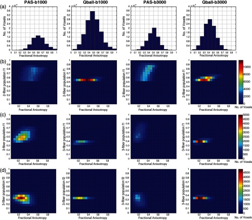
Figure 5 explores both the number of voxels identified along with the FA and peak fraction. Q-ball shows more voxels with single fiber populations than PAS at both $b$ values [Fig. 5(a)]. As the $b$ values increase, PAS exhibits a slight increase in the single fiber voxels while Q-ball finds a substantial decrease. With the two-fiber case, PAS estimates a wide spread of peak fraction (0.5 to 0.8) for a range of FA (0.2 to 0.8), but Q-ball finds a very narrow, peak fraction of (0.5 to 0.6) for a more limited range of FA (0.3 to 0.6) [Fig. 5(b)]. The number of two-fiber voxels moderately increases with $b$ value for PAS and Q-ball. For the three-fiber case, there is substantial decrease in detected fibers with PAS, but an increase with Q-ball. For a $b$ value of $1000\mathrm{s}/{\mathrm{mm}}^2$, PAS finds three fibers for an FA of 0 to 0.6, but for a $b$ value of $3000\mathrm{s}/{\mathrm{mm}}^2$, PAS detects three fibers only $\mathrm{FA}<0.4$. For Q-ball, the FA range remains the same (FA in 0 to 0.5) with a peak fraction of approximately one-third for both $b$ values [Figs. 5(c) and 5(d)].

Fig. 5.

Peak fraction of PAS and Q-ball across eleven single scans for $b$-values of $1000\mathrm{s}/{\mathrm{mm}}^2$ and $3000\mathrm{s}/{\mathrm{mm}}^2$. (a) Histogram depicting the number of voxels mapped as a function of FA. (b) $f1$ of two fiber populations as function of FA with number of voxels as the third dimension. (c) $f1$ of three fiber populations as function of FA with number of voxels as the third dimension. (b) $f2$ of three fiber populations as function of FA with number of voxels as the third dimension.

The single fiber cases exhibit SAE less than multifiber cases for both PAS and Q-ball (Fig. 6). SAE decreases with increased FA for all scenarios. PAS shows lower SAE than Q-ball [Figs. 6(a) versus 6(b) and 6(c) versus 6(d)]. Interestingly, SAEs are lower for the three crossing fibers relative to the two crossing fibers. Yet, note that 7836 and 661 voxels were detected with three fibers for PAS and Q-ball at $b$ value of $1000\mathrm{s}/{\mathrm{mm}}^2$ while they were 2941 and 816 at $b$ value of $3000\mathrm{s}/{\mathrm{mm}}^2$, respectively. Figure 5 presents a qualitative comparison.

Fig. 6.

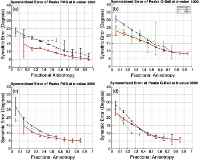
SAE is shown for (a) PAS at $b$ value of $1000\mathrm{s}/{\mathrm{mm}}^2$, (b) Q-ball at $b$ value of $1000\mathrm{s}/{\mathrm{mm}}^2$, (c) PAS at $b$ value of $3000\mathrm{s}/{\mathrm{mm}}^2$, and (d) Q-ball at $b$ value of $3000\mathrm{s}/{\mathrm{mm}}^2$. Error bars represent standard deviation across the bin.

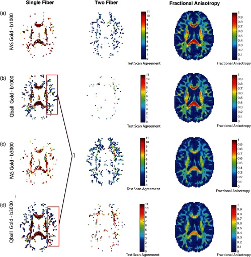
Figure 8 compares the gold standard estimates from PAS to the individual estimates from Q-ball and vice versa. SF follows the same trend for all four scenarios for the single fiber population. For the single fiber case, SF is higher when the PAS is treated as the baseline [red curves: Figs. 8(a) versus 8(c) and 8(b) versus 8(d)]. Yet, for the two-fiber model, Q-ball ground truth generally agrees with PAS at high $b$ value ($>0.5$), but a substantial fraction ($\sim 80\%$) of PAS two-fiber cases are not seen in Q-ball [black curves: Figs. 8(a) versus 8(c) and 8(b) versus 8(d)]. The three-fiber cases are not consistent for either the baseline or $b$-value scenario (blue curves: Fig. 8). We can appreciate these levels of agreement qualitatively in Fig. 9. The major white matter tracts have single fiber detected and have high SF with both approaches used as gold standards (Fig. 9, first column). The impact of the number of voxels shown with two fibers on the overall SF is shown in the second column of Fig. 9.

Fig. 8.

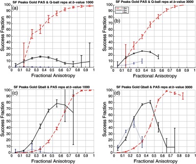
(a) SF gold standard model PAS and test models Q-ball at $b$ value of $1000\mathrm{s}/{\mathrm{mm}}^2$. (b) SF gold standard model PAS and test models Q-ball at $b$ value of $3000\mathrm{s}/{\mathrm{mm}}^2$. (c) SF gold standard model $Q$ ball and test models PAS at $b$ value of $1000\mathrm{s}/{\mathrm{mm}}^2$. (d) SF gold standard model Q-ball and test models PAS at $b$ value of $3000\mathrm{s}/{\mathrm{mm}}^2$. Error bars represent standard deviation across the bin.

Fig. 9.

Middle-axial slice spatial map for intramodel comparison. (a) PAS gold standard model and Q-ball test models at $b$ value $1000\mathrm{s}/{\mathrm{mm}}^2$. (b) Q-ball gold standard model and PAS test models at $b$ value $1000\mathrm{s}/{\mathrm{mm}}^2$. (c) PAS gold standard model and Q-ball test models at $b$ value $3000\mathrm{s}/{\mathrm{mm}}^2$. (d) Q-ball gold standard model and PAS test models at $b$ value $3000\mathrm{s}/{\mathrm{mm}}^2$. (1) False positives being detected by PAS.

5. Discussion

This study focuses on capturing the differences between PAS and Q-ball interpretations of a single acquisition type using the established best practices. We interpret the differences observed in the results to be fundamentally attributed to algorithms and hence discuss the relative sensitivity/reproducibility of each approach. Note that the observed differences between Q-ball and PAS may arise not only from the data model but also from their dependencies on experimental factors (e.g., noise level and angular sampling), on the selection of reconstruction/model parameters (e.g., order/radius), peak determination algorithm parameters. The data has been made freely available at the official NITRC website.

In the literature, Q-ball has been shown to detect crossing angles in multifiber regions down to 45 deg at $b$ values of $8000\mathrm{s}/{\mathrm{mm}}^2$. Given sufficient SNR using high quality phantom data, Q-ball improves in accuracy with $b$ values $>4000\mathrm{s}/{\mathrm{mm}}^2$.¹² Typically, these $b$ values are not clinically feasible. Crossing fiber angles have been detected with Q-ball for FA less than 0.4.¹¹ Meanwhile, PAS resolves greater crossing fiber populations on sparse diffusion data and is able to resolve crossing fibers at lower $b$ values, which are clinically feasible.¹⁰

Herein, we find that both methods perform well when self-comparing each single scan with concatenated multiple single scans (gold standard model). Specifically, both methods work well on single fiber population scenarios (however, this is not the application for which the methods were designed to address) (Fig. 4).^1,7 However, Q-ball performs better than PAS for single fiber scenarios, which is interesting because it is probable that PAS is detecting false positives. Comparing Figs. 4 and 6, we see that specifically for lower FA there is high standard deviation, which is indicative of the false positives for PAS. Q-ball performs consistently for this scenario.

With the evaluated imaging sequences, Q-ball and PAS reliably detect multiple fibers only for crossing regions with no more than two fiber populations (Fig. 4). Note that PAS and Q-ball both show low reproducibility for extreme FA values, which is a likely an artifact. The inference is that the detection of fiber population might not be accurate. At high values of FA, it is more probable that single fiber populations would be expected rather than two fiber populations, while the lower FA regions show disagreement for two fiber populations, which is not as extreme as for higher FA values. Suggestively, it could be noise that is making the methods underperform in those regions. It is also possible that the methods are not able to resolve more complex architecture, which might be present in the lower anisotropic regions as there is evidence of very low reproducibility in three fiber population regions or more. Comparison with histological validation may indicate which methods are more accurate in regions of disagreement.^36,37 It is likely that usage of these voxels might lead to spurious tracts or false continuations.

Comparing Figs. 4 and 6, we find an interesting difference. The SAE (Fig. 6) shows that most of the errors detected for three-fiber populations are less than the two-fiber population scenario. Yet this is contradicted by the SF (Fig. 4), which shows us that there is hardly any agreement for three-fiber scenarios. Though our analysis suggests that they are not reproducible, there might be a possibility to improve them and increase their reproducibility. Robust fitting of HARDI methods with removal of outlier volumes could lead to improvements.

The peak fractions of Q-ball show a self-consistent, but distinct, value in most scenarios (Fig. 5). While PAS shows them consistently as well but across a wider range, it can be expected from Q-ball that they will be consistent values because a smooth function (ODF) has been normalized. While PAS is a spikier function and hence the wider range of fiber fraction. Characterization of the reconstruction of PAS and ODF may lead to a better understanding but it is beyond the scope of this article, which deals with fiber population and their angular error. A deeper understanding of the differences between ODF and FOD methods is needed, in particular peak fractions lead to quite different interpretations for the different approaches. This is not surprising as the ODF function is quite smooth and not intended to directly model the fiber fraction. For clinical $b$ values ($\sim 1000\mathrm{s}/{\mathrm{mm}}^2$), PAS offers advantages for sensitivity and reproducibility. Q-ball can achieve similar reproducibility performance as PAS given moderate increases in SNR or directions.¹² For higher $b$ values, Q-ball detects more detailed microarchitecture in the brain (Fig. 5) at the higher $b$ value, which implies more voxels detected with crossing fibers. This is supported by the fact that SAE is lower for single and two fiber populations for higher $b$ values (Fig. 6). PAS appears to be a more reasonable choice given higher reproducibility of crossing fiber majorly of the two fiber populations (Figs. 4 and Fig. 6). However, care should be taken in interpretation of both methods as to which regions they are applied as both methods are unstable at the extreme of FA (Fig. 4).

Prior conference analysis of the data²⁹ showed that PAS resolves crossing fibers more consistently than Q-ball at moderate and higher crossing angles. Accuracy and consistency for both Q-ball and PAS have been shown to increase with increasing SNR (our empirical data is low SNR),^8,12 but the observed methodological effects are not mitigated by large quantities of data as indicated as at the comparison between gold standard models computing using all available data (Figs. 4 and 6). In Ref. 8, PAS was consistent in all cases with $\mathrm{SNR}>16$, but for Q-ball to reach this level of consistent/accuracy $\mathrm{SNR}>24$ (which ours is not, and is not often seen in clinical scans). Note that the SNR of the presented data were 11.828 in the centrum semiovale (WM), in the peripheral white matter, and 5.838 in the cortical gray matter in the b0 images. Also shown are values of single b0 equivalent as our scanner provides with an average of 10 b0’s for a b0 (Tables 1 and 2). Hence, single b0 equivalent is (SNR calculated)/$\sqrt{10}$. The SNR has been calculated using Reeder’s difference method.³⁸ PAS accuracy and consistency is better than Q-ball for crossing fibers at our low/clinically feasible SNR regime, Q-ball is more consistent than PAS in single fiber regions at a lower SNR. This is interesting to note, probably due to the false positives in PAS.

Table 1.

Mean SNR and the error observed per session for the acquired dataset.

Session	Mean SNR	Std SNR	Single b0 equivalent
Session 1	32.81	0.1091	10.3768
Session 2	27.84	0.0830	8.8065
Session 3	32.81	0.1091	10.3768

Table 2.

Mean SNR and the error observed across all sessions for the acquired dataset.

Session	Mean SNR	Std SNR	Single b0 equivalent
All sessions	33.12	0.0945	10.47

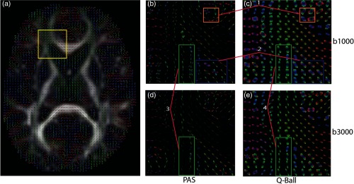
Q-ball shows fanning fiber voxels while PAS detects sharp and narrow peaks as visually evident by the glyphs [see (1) in Fig. 7]. A higher number of crossing fiber voxels is seen for PAS when compared to Q-ball glyphs, which also reinforces the fact that there are more 2 or more fiber voxels for PAS [see (2) in Fig. 7]. Highlighting architectural differences between the two methods. The effect of $b$ value can be seen on both methods as it increases from 1000 to $3000\mathrm{s}/{\mathrm{mm}}^2$. It is evident that fanning of the fiber reduces and peaks become narrower for Q-ball and PAS both [see (3, 4) in Fig. 7]. However, for Q-ball it is beneficial for PAS it is detrimental. It is noticeable qualitatively that the fanning structure being captured by PAS-MRI at $b$ value of $1000\mathrm{s}/{\mathrm{mm}}^2$ is lost once the $b$ value is increased [see (3) in Fig. 7]. This loss of structure is also being quantified by the SAE metric (Fig. 6). The crossing fiber voxels being detected till FA of 0.8 to 0.9 at $b$ value of $1000\mathrm{s}/{\mathrm{mm}}^2$ has dropped to $\mathrm{FA}<0.6$.

Fig. 7.

Enlarged ROI contains genu of corpus callosum and left prefrontal area: (a) Q-ball is shown for the middle axial slice at $b$ value of $3000\mathrm{s}/{\mathrm{mm}}^2$. Enlargements are presented for: (b) PAS at $b$ value $1000\mathrm{s}/{\mathrm{mm}}^2$, (c) Q-ball at $b$ value $1000\mathrm{s}/{\mathrm{mm}}^2$, (d) PAS at $b$ value $3000\mathrm{s}/{\mathrm{mm}}^2$, and (e) Q-ball at $b$ value $3000\mathrm{s}/{\mathrm{mm}}^2$. (1) Structural differences between PAS and Q-ball. (2) Fanning fibers in Q-ball while crossings detected by PAS. (3) Loss of structure for PAS. (4) Reduction in fanning for Q-ball.

At high values of FA ($>0.6$), there is noticeable disagreement between Q-ball and PAS, which is evident even for the two-fiber case (Fig. 8). PAS detects multiple fibers even when the tensor FA is high, which would appear to indicate false positives [Fig. 9, see (1)]. Meanwhile, Q-ball consistently finds a single fiber in cases where the tensor FA is high.

In summary, the analyses for single-fiber populations are in good self-agreement with PAS; however, there is the possibility of false positives. Q-ball performs qualitatively better with fair intermodel agreement. For two-fiber populations, the methods are in fair self-agreement except for extreme high or low FA regions. Overall PAS shows more reproducibility and the intermodel agreement is reasonable for midranges of white matter FA ($0.4<\mathrm{FA}<0.6$). The three-fiber population case shows low self-agreement indicating model instability for both PAS and Q-ball. There is little agreement between both methods in terms of crossing fibers (Figs. 8 and 9). Visually also the agreement is less than expected given crossing fiber regions or two and more fiber population voxels.

Biography

Biographies for the authors are not available.

Disclosures

The authors have no additional relevant financial interests in this manuscript.

References

- 1.Basser P. J., Mattiello J., LeBihan D., “Estimation of the effective self-diffusion tensor from the NMR spin echo,” J. Magn. Reson., Ser. B 103(3), 247–254 (1994).https://doi.org/10.1006/jmrb.1994.1037 [DOI] [PubMed] [Google Scholar]
- 2.Özarslan E., et al. , “Resolution of complex tissue microarchitecture using the diffusion orientation transform (DOT),” NeuroImage 31(3), 1086–1103 (2006).https://doi.org/10.1016/j.neuroimage.2006.01.024 [DOI] [PubMed] [Google Scholar]
- 3.Anderson A. W., “Measurement of fiber orientation distributions using high angular resolution diffusion imaging,” Magn. Reson. Med. 54(5), 1194–1206 (2005).https://doi.org/10.1002/(ISSN)1522-2594 [DOI] [PubMed] [Google Scholar]
- 4.Tournier J.-D., et al. , “Direct estimation of the fiber orientation density function from diffusion-weighted MRI data using spherical deconvolution,” NeuroImage 23(3), 1176–1185 (2004).https://doi.org/10.1016/j.neuroimage.2004.07.037 [DOI] [PubMed] [Google Scholar]
- 5.Jansons K. M., Alexander D. C., “Persistent angular structure: new insights from diffusion magnetic resonance imaging data,” Inverse Prob. 19(5), 1031–1046 (2003).https://doi.org/10.1088/0266-5611/19/5/303 [DOI] [PubMed] [Google Scholar]
- 6.Tuch D. S., “Q‐ball imaging,” Magn. Reson. Med. 52(6), 1358–1372 (2004).https://doi.org/10.1002/(ISSN)1522-2594 [DOI] [PubMed] [Google Scholar]
- 7.Farrell J. A., et al. , “Effects of signal‐to‐noise ratio on the accuracy and reproducibility of diffusion tensor imaging-derived fractional anisotropy, mean diffusivity, and principal eigenvector measurements at 1.5 T,” J. Magn. Reson. Imaging 26(3), 756–767 (2007).https://doi.org/10.1002/(ISSN)1522-2586 [DOI] [PMC free article] [PubMed] [Google Scholar]
- 8.Sweet A., Alexander D., “Reduced encoding persistent angular structure,” in Proc. of Int. Society for Magnetic Resonance in Medicine (2010). [Google Scholar]
- 9.Descoteaux M., et al. , “Regularized, fast, and robust analytical Q‐ball imaging,” Magn. Reson. Med. 58(3), 497–510 (2007).https://doi.org/10.1002/(ISSN)1522-2594 [DOI] [PubMed] [Google Scholar]
- 10.Alexander D., “A comparison of Q-ball and PASMRI on sparse diffusion MRI data,” in Proc. of Int. Society for Magnetic Resonance in Medicine (2004). [Google Scholar]
- 11.Gorczewski K., Mang S., Klose U., “Reproducibility and consistency of evaluation techniques for HARDI data,” Magn. Reson. Mater. Phys. Biol. Med. 22(1), 63–70 (2009).https://doi.org/10.1007/s10334-008-0144-0 [DOI] [PubMed] [Google Scholar]
- 12.Cho K.-H., et al. , “Evaluation of the accuracy and angular resolution of Q-ball imaging,” Neuroimage 42(1), 262–271 (2008).https://doi.org/10.1016/j.neuroimage.2008.03.053 [DOI] [PubMed] [Google Scholar]
- 13.Alexander D. C., “Multiple‐fiber reconstruction algorithms for diffusion MRI,” Ann. N.Y. Acad. Sci. 1064(1), 113–133 (2005).https://doi.org/10.1196/annals.1340.018 [DOI] [PubMed] [Google Scholar]
- 14.Parker G. J., Alexander D. C., “Probabilistic anatomical connectivity derived from the microscopic persistent angular structure of cerebral tissue,” Philos. Trans. R. Soc. Lond. B: Biol. Sci. 360(1457), 893–902 (2005).https://doi.org/10.1098/rstb.2005.1639 [DOI] [PMC free article] [PubMed] [Google Scholar]
- 15.Seunarine K. K., et al. “Exploiting peak anisotropy for tracking through complex structures,” in IEEE 11th Int. Conf. on Computer Vision, ICCV 2007, IEEE (2007).https://doi.org/10.1109/ICCV.2007.4409168 [Google Scholar]
- 16.Yo T.-S., et al. “Quantifying brain connectivity: a comparative tractography study,” in Int. Conf. on Medical Image Computing and Computer-Assisted Intervention, Springer; (2009). [DOI] [PubMed] [Google Scholar]
- 17.Descoteaux M., Deriche R., “From local Q-ball estimation to fibre crossing tractography,” in Handbook of Biomedical Imaging, Paragios N., Duncan J., Ayache N., Eds., pp. 455–473, Springer, Boston, Massachusetts: (2015). [Google Scholar]
- 18.Xie S., et al. , “How does B-value affect HARDI reconstruction using clinical diffusion MRI data?” PLoS One 10(3), e0120773 (2015).https://doi.org/10.1371/journal.pone.0120773 [DOI] [PMC free article] [PubMed] [Google Scholar]
- 19.Perrin M., et al. , “Validation of Q-ball imaging with a diffusion fibre-crossing phantom on a clinical scanner,” Philos. Trans. R. Soc. Lond. B: Biol. Sci. 360(1457), 881–891 (2005).https://doi.org/10.1098/rstb.2005.1650 [DOI] [PMC free article] [PubMed] [Google Scholar]
- 20.Dayan M., Kreutzer S., Clark C. A., “Tractography of the optic radiation: a repeatability and reproducibility study,” NMR Biomed. 28(4), 423–431 (2015).https://doi.org/10.1002/nbm.3266 [DOI] [PubMed] [Google Scholar]
- 21.Andersson J. L., Skare S., Ashburner J., “How to correct susceptibility distortions in spin-echo echo-planar images: application to diffusion tensor imaging,” Neuroimage 20(2), 870–888 (2003).https://doi.org/10.1016/S1053-8119(03)00336-7 [DOI] [PubMed] [Google Scholar]
- 22.Andersson J. L., Sotiropoulos S. N., “Non-parametric representation and prediction of single-and multi-shell diffusion-weighted MRI data using Gaussian processes,” Neuroimage 122, 166–176 (2015).https://doi.org/10.1016/j.neuroimage.2015.07.067 [DOI] [PMC free article] [PubMed] [Google Scholar]
- 23.Jenkinson M., Smith S., “A global optimisation method for robust affine registration of brain images,” Med. Image Anal. 5(2), 143–156 (2001).https://doi.org/10.1016/S1361-8415(01)00036-6 [DOI] [PubMed] [Google Scholar]
- 24.Holmes C. J., et al. , “Enhancement of MR images using registration for signal averaging,” J. Comput. Assisted Tomogr. 22(2), 324–333 (1998).https://doi.org/10.1097/00004728-199803000-00032 [DOI] [PubMed] [Google Scholar]
- 25.Tustison N. J., et al. , “N4ITK: improved N3 bias correction,” IEEE Trans. Med. Imaging 29(6), 1310–1320 (2010).https://doi.org/10.1109/TMI.2010.2046908 [DOI] [PMC free article] [PubMed] [Google Scholar]
- 26.Avants B. B., Tustison N., Song G., “Advanced normalization tools (ANTS),” Insight J. 2, 1–35 (2009). [Google Scholar]
- 27.Avants B. B., et al. , “Symmetric diffeomorphic image registration with cross-correlation: evaluating automated labeling of elderly and neurodegenerative brain,” Med. Image Anal. 12(1), 26–41 (2008).https://doi.org/10.1016/j.media.2007.06.004 [DOI] [PMC free article] [PubMed] [Google Scholar]
- 28.Asman A. J., Landman B. A., “Formulating spatially varying performance in the statistical fusion framework,” IEEE Trans. Med. Imaging 31(6), 1326–1336 (2012).https://doi.org/10.1109/TMI.2012.2190992 [DOI] [PMC free article] [PubMed] [Google Scholar]
- 29.Asman A. J., Landman B. A., “Non-local statistical label fusion for multi-atlas segmentation,” Med. Image Anal. 17(2), 194–208 (2013).https://doi.org/10.1016/j.media.2012.10.002 [DOI] [PMC free article] [PubMed] [Google Scholar]
- 30.Freund Y., Schapire R. E., “A desicion-theoretic generalization of on-line learning and an application to boosting,” in European Conf. on Computational Learning Theory, Springer; (1995). [Google Scholar]
- 31.Klein A., et al. , “Open labels: online feedback for a public resource of manually labeled brain images,” in 16th Annual Meeting for the Organization of Human Brain Mapping (2010). [Google Scholar]
- 32.Schilling K. G., et al. , “Empirical consideration of the effects of acquisition parameters and analysis model on clinically feasible Q-ball imaging,” Magn. Reson. Imaging 40, 62–74 (2017).https://doi.org/10.1016/j.mri.2017.04.007 [DOI] [PMC free article] [PubMed] [Google Scholar]
- 33.Cook P., et al. , “Camino: open-source diffusion-MRI reconstruction and processing,” in 14th Scientific Meeting of the Int. Society for Magnetic Resonance in Medicine, Seattle, Washington, USA (2006). [Google Scholar]
- 34.Alexander D. C., “Maximum entropy spherical deconvolution for diffusion MRI,” in Biennial Int. Conf. on Information Processing in Medical Imaging, Christensen G. E., Sonka M., Eds., pp. 76–87, Springer, Berlin, Heidelberg: (2005). [DOI] [PubMed] [Google Scholar]
- 35.NITRC, “https://www.nitrc.org/.
- 36.Schilling K., et al. , “Reproducibility and variation of diffusion measures in the squirrel monkey brain, in vivo and ex vivo,” Magn. Reson. Imaging 35, 29–38 (2017).https://doi.org/10.1016/j.mri.2016.08.015 [DOI] [PMC free article] [PubMed] [Google Scholar]
- 37.Schilling K., et al. , “Comparison of 3D orientation distribution functions measured with confocal microscopy and diffusion MRI,” Neuroimage 129, 185–197 (2016).https://doi.org/10.1016/j.neuroimage.2016.01.022 [DOI] [PMC free article] [PubMed] [Google Scholar]
- 38.Reeder S. B., et al. , “Practical approaches to the evaluation of signal‐to‐noise ratio performance with parallel imaging: application with cardiac imaging and a 32‐channel cardiac coil,” Magn. Reson. Med. 54(3), 748–754 (2005).https://doi.org/10.1002/(ISSN)1522-2594 [DOI] [PubMed] [Google Scholar]