Association testing of bisulfite-sequencing methylation data via a Laplace approximation

Abstract

Motivation

Epigenome-wide association studies can provide novel insights into the regulation of genes involved in traits and diseases. The rapid emergence of bisulfite-sequencing technologies enables performing such genome-wide studies at the resolution of single nucleotides. However, analysis of data produced by bisulfite-sequencing poses statistical challenges owing to low and uneven sequencing depth, as well as the presence of confounding factors. The recently introduced Mixed model Association for Count data via data AUgmentation (MACAU) can address these challenges via a generalized linear mixed model when confounding can be encoded via a single variance component. However, MACAU cannot be used in the presence of multiple variance components. Additionally, MACAU uses a computationally expensive Markov Chain Monte Carlo (MCMC) procedure, which cannot directly approximate the model likelihood.

Results

We present a new method, Mixed model Association via a Laplace ApproXimation (MALAX), that is more computationally efficient than MACAU and allows to model multiple variance components. MALAX uses a Laplace approximation rather than MCMC based approximations, which enables to directly approximate the model likelihood. Through an extensive analysis of simulated and real data, we demonstrate that MALAX successfully addresses statistical challenges introduced by bisulfite-sequencing while controlling for complex sources of confounding, and can be over 50% faster than the state of the art.

Availability and Implementation

The full source code of MALAX is available at https://github.com/omerwe/MALAX.

Supplementary information

Supplementary data are available at Bioinformatics online.

1 Introduction

In recent years, epigenetic variation has proven to be an important factor in many traits and diseases (Bird, 2007). One of the most prominent sources of epigenetic variation is differential DNA methylation (Jones, 2012). Currently, the predominant technology for measuring methylation levels is based on methylation arrays, which can probe a specific list of sites. However, the recently emerging bisulfite-sequencing technology enables measuring methylation levels across the entire genome (Cokus et al., 2008). In spite of the clear advantages, testing for associations between methylation patterns and phenotypes via bisulfite-sequencing data is hindered by several challenges.

The main challenge in the analysis of bisulfite-sequencing data is their typically low and uneven sequencing depth. Specifically, the proportion of the number of methylated reads to the total number of reads is an unreliable measure of the true methylation level, when the total number of reads is small. Consequently, naive application of regression models for such data leads to loss of power and to spurious results (Sun et al., 2014). To circumvent this difficulty, several methods proposed treating the phenotype as an explanatory variable and the methylation sites as beta-binomial (BB) distributed response variables (Dolzhenko and Smith, 2014; Feng et al., 2014; Sun et al., 2014). The use of a BB distribution accounts for both the binomial nature of the methylation levels and for their tendency to be highly overdispersed relative to a standard binomial distribution.

Although the aforementioned methods successfully account for independent overdispersion, methylation counts of different individuals are often correlated owing to confounding factors such as population structure, cryptic relatedness or batch effects in the data (Lea et al., 2015). Such confounding factors must be accounted for to prevent spurious findings. Linear mixed models (LMMs) are often used to control for confounding in genetic studies (Yang et al., 2014), but similarly to other regression models, LMMs suffer from loss of power and spurious results in the presence of bisulfite-sequencing data (Lea et al., 2015). To address this challenge, Mixed model Association for Count data via data AUgmentation (MACAU) (Lea et al., 2015) combines the idea of treating methylation sites as response variables, with a generalized linear mixed model (GLMM) that can control for confounding.

A severe limitation of GLMMs is that numerical likelihood evaluation is computationally infeasible in typical settings. To overcome this limitation, MACAU assigns a prior distribution to the model parameters and then estimates their posterior distribution via MCMC. The posterior mean and variance estimates of the effect of the phenotype on a certain site are then used to test for association, by treating them as maximum likelihood estimates (MLEs) and using them in a Wald test context.

Although MACAU addresses the computational infeasibility limitation, the proposed MCMC approach suffers from two caveats. First and foremost, MACAU cannot be used in the presence of multiple variance components, because it uses an approximation that specifically exploits the structure of its probabilistic model when there is only a single variance component (in addition to the variance component associated with the identity matrix). In recent years it has been shown that it is often beneficial to use multiple variance components to control for multiple sources of confounding. For example, Widmer et al. (2014) suggested using two variance components to improve the model fit; Chen et al. (2016) used three variance components to control for genetic relatedness as well as household and block group membership; Cohen et al. (2016) used two variance components to control for both genetic relatedness and for experimental variability; Powell et al. (2013) used two variance components corresponding to additive and dominance effects. In the context of Epigenome-wide association studies (EWASs), it can be beneficial to control for genetic similarity as well as methylation similarity, which can for example capture confounding due to cell type composition (Zou et al., 2014).

A second caveat of the proposed MCMC approach is the need to carry out convergence diagnostics and fine-tune many parameters, which hinders the use of MCMC methods in practice.

Here we present Mixed model Association via a Laplace ApproXimation (MALAX), which directly approximates the likelihood of the GLMM used by MACAU via a Laplace approximation (Rasmussen and Williams, 2006). Briefly, MALAX approximates the conditional distribution of the logit of the methylation levels given the data as a multivariate normal distribution, by using a second order Taylor expansion. This approximation enables a fast analytical approximation of the MLEs of all parameters, allowing MALAX to successfully address the caveats above: MALAX can be used with multiple variance components, it does not assume the existence of a prior distribution of the model parameters, and it does not require parameter fine-tuning. Additionally, MALAX can be over 50% faster than the state of the art.

In order to evaluate MALAX we carry out extensive simulations of studies with diverse sources of confounding. We additionally demonstrate the advantages of MALAX in an analysis of 50 baboons with multiple variance components, which was not possible using previous methods. Our simulations and real data analysis indicate that MALAX has high power to discover phenotype-epigenetic associations, while controlling for diverse sources of confounding.

2 Materials and methods

2.1 Methods overview

We begin by providing an overview of association testing in the presence of bisulfite-sequencing data. Consider a dataset of n individuals with measured phenotypes, covariates, read counts and methylated read counts. We are interested in testing the null hypothesis that the proportion of methylated reads at site j is independent of the phenotype.

A naive approach is to treat the observed proportion of methylated reads at site j as an additional covariate and test for association between this covariate and the phenotype via a regression model. Specifically, assuming a quantitative phenotype and denoting $\mathit{x}={[x_1,\dots ,x_n]}^T$ as a vector of observed phenotypes, ${\mathit{y}}^j={[y_1^j,\dots ,y_n^j]}^T$ and ${\mathit{r}}^j={[r_1^j,\dots ,r_n^j]}^T$ as vectors with the number of methylated reads and the total number of reads for site j, respectively, and $\mathit{W}={[{\mathit{w}}_1,\dots ,{\mathit{w}}_n]}^T$ as a matrix of covariates including an intercept, (where each element ${\mathit{w}}_i$ is a vector of c covariates for individual i), a naive regression model is defined as follows:

$$\mathit{x}=\mathit{W\alpha }+\left({\mathit{y}}^j/{\mathit{r}}^j\right)\beta +\epsilon .$$ (1)

Here, $\epsilon \sim \mathcal{N}\left(\mathbf{0},{\sigma }_e^2\mathit{I}\right)$ is a vector of independent normally distributed residuals with variance ${\sigma }_e^2$, $\left({\mathit{y}}^j/{\mathit{r}}^j\right)={[y_1^j/r_1^j,\dots ,y_n^j/r_n^j]}^T$ is a vector of methylation levels, $\mathit{\alpha }={[{\alpha }_1,\dots ,{\alpha }_c]}^T$ is a vector of fixed effects, and β is the fixed effect of the methylation level. Association testing amounts to testing the null hypothesis ${\mathcal{H}}_0:\beta =0$. The above model can be extended to account for complex sources of confounding by using a LMM, which consists of changing the distribution of $\epsilon$ to $\epsilon \sim \mathcal{N}(\mathbf{0},{\sum }_{v=1}^V{\sigma }_v^2{\mathit{K}}_v+{\sigma }_e^2\mathit{I})$, where ${\mathit{K}}_v$ is an n × n matrix describing the effect of the vth source of confounding, and ${\sigma }_v^2$ is the vth variance component.

Unfortunately, the observed proportions encoded in the vector ${\mathit{y}}^j/{\mathit{r}}^j$ are unreliable estimators of the true proportions when ${\mathit{r}}^j$ contains small numbers, which can in turn lead to loss of power and to spurious results (Lea et al., 2015). A common solution is to treat the phenotype as a covariate and the observed number of reads as a response variable, which enables to explicitly model the binomial nature of the methylation levels. We now present the statistical model of MALAX and MACAU, which adopts this approach in the framework of a GLMM.

2.2 Statistical model

MALAX models the distribution of $y_i^j$ conditional on all the other variables via a binomial GLMM as follows:

$$\begin{array}{l}{y}_i^j\hspace{0.17em}|\hspace{0.17em}{r}_i^j,x_i,{\mathit{w}}_i\sim \text{Bin}\left(r_i^j,{\pi }_i^j\right)\\ {\pi }_i^j={\left(1+\text{exp}\hspace{0.17em}\left(-l_i\right)\right)}^{-1}\\ \mathit{l}\sim \mathcal{N}\left(\mathit{W}\alpha +\mathit{x}\beta ,{\sum }_{v=1}^V{\sigma }_v^2{\mathit{K}}_v+{\sigma }_e^2\mathit{I}\right).\end{array}$$ (2)

Here, ${\pi }_i^j$ is the methylation probability of a probe coming from site j in individual i, and $\mathit{l}={[l_1,\dots ,l_n]}^T$ is the vector of the logits of these probabilities. The variance component ${\sigma }_e^2$ accounts for independent over-dispersion, which describes the observation that the variance of methylation levels across different individuals is often much larger than expected under a binomial model.

A natural interpretation of this model is that every individual i is associated with a latent random variable l_i which is affected by her covariates and genetic variants, such that larger values of l_i lead to higher methylation levels. In this respect, the model is similar to the well-known liability threshold model often employed in case-control studies (Weissbrod et al., 2015), wherein every individual is associated with a latent liability value. If ${\mathit{K}}_v$ is a matrix of inner-products of normalized genetic vectors, it encodes the assumption that genetic variants exert a linear effect on l_i, similarly to the assumption often employed in standard LMMs.

Association testing consists of testing the null hypothesis ${\mathcal{H}}_0:\beta =0$, and can be carried out via a Wald test, which requires computing the MLE of the model parameters. The log likelihood function is given by:

$$\ell \left(\mathit{\alpha },\beta ,{\sigma }_1^{\mathrm{2}},\dots ,{\sigma }_V^2,{\sigma }_e^2\right)=\text{log}\hspace{0.17em}\int P\left(\mathit{l}\right){\prod }_{i=1}^{n}P\left(y_i^j\hspace{0.17em}|\hspace{0.17em}{l}_i,r_i^j\right)d\mathit{l},$$ (3)

where we omitted conditioning l on the observed variables and on the model parameters for brevity. Equation (3) demonstrates that likelihood evaluation requires numerically evaluating an n-dimensional integral, which scales exponentially with n when using state of the art algorithms, such as adaptive Gauss-Kronrod quadrature (Kahaner et al., 1989). To circumvent this difficulty, MACAU adopts a Bayesian framework by first assigning a prior distribution to the fixed effects and variance components, and then sampling parameter values from their posterior distribution. In contrast, MALAX does not assume that the parameters have a prior distribution, and instead directly approximates the likelihood via a Laplace approximation.

2.3 Laplace approximation

The underlying idea behind MALAX is that the conditional density $P\left(\mathit{l}\hspace{0.17em}|\hspace{0.17em}\mathit{x},\mathit{W},{\mathit{y}}^j,{\mathit{r}}^j\right)$ can be approximated to follow a multivariate Gaussian via a second order Taylor expansion. Under this approximation, the log likelihood can be approximated as follows:

$$\begin{array}{l}\ell \left(\mathit{\alpha },\beta ,{\sigma }_1^{\mathrm{2}},\dots ,{\sigma }_V^2,{\sigma }_e^2\right)\approx \\ -\frac{1}{2}\left({\left(\widehat{\mathit{l}}-\mathit{m}\right)}^{\mathrm{T}}\nabla \hspace{0.17em}\text{log}\hspace{0.17em}P\left({\mathit{y}}^j|\mathit{l}\right){|}_{\mathit{l}=\widehat{\mathit{l}}}\right)-\frac{1}{2}\text{log}\hspace{0.17em}\left|\mathit{GA}\right|+\text{log}\hspace{0.17em}P\left({\mathit{y}}^j|\widehat{\mathit{l}}\right).\end{array}$$ (4)

Here, $\widehat{\mathit{l}}={\text{argmax}}_{\mathit{l}}P\left(\mathit{l}\hspace{0.17em}|\hspace{0.17em}\mathit{x},\mathit{W},{\mathit{y}}^j,{\mathit{r}}^j\right),\hspace{0.17em}\mathit{G}={\sum }_{v=1}^V{\sigma }_v^2{\mathit{K}}_v+{\sigma }_e^2\mathrm{I}$ is the overall covariance matrix, $\mathit{m}=\mathit{W\alpha +x\beta }$ is the mean of l, $\nabla \hspace{0.17em}\text{log}\hspace{0.17em}P\left({\mathit{y}}^j|\mathit{l}\right){|}_{\mathit{l}=\widehat{\mathit{l}}}$ is the gradient of $\text{log}\hspace{0.17em}P\left({\mathit{y}}^j|\mathit{l}\right)$ with respect to l, evaluated at $\mathit{l}=\widehat{\mathit{l}}$, and $\mathit{A}\triangleq -\nabla \nabla \hspace{0.17em}\text{log}\hspace{0.17em}\mathrm{P}\left(\mathit{l}\hspace{0.17em}|\hspace{0.17em}\mathit{x},\mathit{W},{\mathit{y}}^j,{\mathit{r}}^j\right){|}_{\mathit{l}=\widehat{\mathit{l}}}$ is the Hessian of the negative logarithm of the conditional density of l with respect to l, evaluated at $\mathit{l}=\widehat{\mathit{l}}$.

A brief sketch of the derivation of Equation (4) is now provided, with a longer description available in (Rasmussen and Williams, 2006). First, we apply a second order Taylor expansion to the logarithm of $P\left(\mathit{l},{\mathit{y}}^j\hspace{0.17em}|\hspace{0.17em}\mathit{x},\mathit{W},{\mathit{r}}^j\right)$ around $\widehat{\mathit{l}}$ as follows:

$$\begin{array}{l}\hspace{0.17em}\text{log}\hspace{0.17em}P\left(\mathit{l},{\mathit{y}}^j\hspace{0.17em}|\hspace{0.17em}\mathit{x},\mathit{W},{\mathit{r}}^j\right)\\ \approx \hspace{0.17em}\text{log}\hspace{0.17em}P\left(\mathit{l}=\widehat{\mathit{l}},{\mathit{y}}^j\hspace{0.17em}|\hspace{0.17em}\mathit{x},\mathit{W},{\mathit{r}}^j\right)-\frac{1}{2}{\left(\mathit{l}-\widehat{\mathit{l}}\right)}^T\mathit{A}\left(\mathit{l}-\widehat{\mathit{l}}\right).\end{array}$$ (5)

Using this approximation, the log likelihood can be approximated analytically as follows:

$$\begin{array}{l}\ell \left(\mathit{\alpha },\beta ,{\sigma }_1^{\mathrm{2}},\dots ,{\sigma }_V^2,{\sigma }_e^2\right)=\text{log}\hspace{0.17em}P\left({\mathit{y}}^j|\mathit{x},\mathit{W},{\mathit{r}}^j\right)\\ \approx \hspace{0.17em}\text{log}\hspace{0.17em}[P\left(\mathit{l}=\widehat{\mathit{l}},{\mathit{y}}^j|\mathit{x},\mathit{W},{\mathit{r}}^j\right)\int \hspace{0.17em}\text{exp}\hspace{0.17em}\left(-\frac{1}{2}{\left(\mathit{l}-\widehat{\mathit{l}}\right)}^T\mathit{A}\left(\mathit{l}-\widehat{\mathit{l}}\right)\right)d\mathit{l}]\\ =\text{log}\hspace{0.17em}[P\left(\mathit{l}=\widehat{\mathit{l}},{\mathit{y}}^j|\mathit{x},\mathit{W},{\mathit{r}}^j\right){\left(2\pi \right)}^{n/2}{\left|\mathit{A}\right|}^{-\frac{1}{2}}]\\ =-\frac{1}{2}{\left(\widehat{\mathit{l}}-\mathit{m}\right)}^T{\mathit{G}}^{-1}\left(\widehat{\mathit{l}}-\mathit{m}\right)-\frac{1}{2}\text{log}\hspace{0.17em}\left|\mathrm{GA}\right|+\text{log}\hspace{0.17em}P\left({\mathit{y}}^j|\widehat{\mathit{l}}\right)\\ =-\frac{1}{2}{\left(\widehat{\mathit{l}}-\mathit{m}\right)}^T\nabla \hspace{0.17em}\text{log}\hspace{0.17em}P\left({\mathit{y}}^j|\mathit{l}\right){|}_{\mathit{l}=\widehat{\mathit{l}}}-\frac{1}{2}\text{log}\hspace{0.17em}\left|\mathrm{GA}\right|+\text{log}\hspace{0.17em}P\left({\mathit{y}}^j|\widehat{\mathit{l}}\right).\end{array}$$ (6)

The second equality can be verified by noting that the integral is equal to the reciprocal of the normalizing constant of a multivariate normal distribution with mean vector $\widehat{\mathit{l}}$ and covariance matrix ${\mathit{A}}^{-1}$. The third equality is derived by using the definition of $P\left(\mathit{l}=\widehat{\mathit{l}},{\mathit{y}}^j|\mathit{x},\mathit{W},{\mathit{r}}^j\right)$ and some algebra. The fourth equality uses the following equation:

$$\nabla \hspace{0.17em}\text{log}\hspace{0.17em}P\left(\mathit{l},{\mathit{y}}^j|\mathit{x},\mathit{W},{\mathit{r}}^j\right)=\nabla \hspace{0.17em}\text{log}\hspace{0.17em}P\left({\mathit{y}}^j|\mathit{l}\right)-{\mathit{G}}^{-1}\left(\mathit{l}-\mathit{m}\right),$$ (7)

and the fact that the above equation is equal to 0 by definition when $\mathit{l}=\widehat{\mathit{l}}$.

The computation of $\widehat{\mathit{l}}$ can be performed via Newton–Raphson iterations, which require inverting the Hessian of $\text{log}\hspace{0.17em}P\left(\mathit{l},{\mathit{y}}^j|\mathit{x},\mathit{W},{\mathit{r}}^j\right)$ with respect to l. Additionally, the likelihood approximation requires evaluating the determinant of the matrix AG. Both operations scale cubically with n under standard implementations. Hence, the computational complexity of the algorithm is $\mathcal{O}\left(n^3\right)$. The number of cubic operations required for each methylation site depends on the number of iterations required for convergence of the Newton-Raphson algorithm and of the optimization scheme, and was typically around 50 in our implementation.

2.4 Testing for association

MALAX tests for association between a phenotype vector x and a vector of methylation counts ${\mathit{y}}^j$ by attempting to reject the null hypothesis ${\mathcal{H}}_0:\beta =0$ via a Wald test. The test statistic is given by $T={\widehat{\beta }}^2/\text{var}\left(\widehat{\beta }\right)$, where $\widehat{\beta }$ is the MLE of β, and asymptotically follows a ${\chi }^2$ distribution with one degree of freedom under the null hypothesis. MALAX estimates $\text{var}\left(\widehat{\beta }\right)$ via the diagonal entry corresponding to β in the inverse of the Hessian of the log likelihood. MALAX approximates the Hessian via finite differences.

2.5 Gradient computation

The gradient of the approximate log likelihood above is required both for approximating the Hessian and for the maximum likelihood estimation procedure. A subtle point that requires consideration is that while the quantities G and m depend explicitly on the model parameters, the quantities $\widehat{\mathit{l}}$ and A also implicitly depend on these parameters. We therefore divide the partial derivative according to each parameter θ (which can represent variance components or fixed effects) into its explicit and implicit components, by using the chain rule as follows:

$$\begin{array}{l}\frac{\partial \hspace{0.17em}\text{log}\hspace{0.17em}P\left({\mathit{y}}^j|\mathit{x},\mathit{W},{\mathit{r}}^j\right)}{\partial \theta }\\ =\frac{\partial L_1}{\partial {\theta }_{\text{explicit}}}+{\sum }_{i=1}^n\frac{\partial \hspace{0.17em}\text{log}\hspace{0.17em}P\left({\mathit{y}}^j|\mathit{x},\mathit{W},{\mathit{r}}^j\right)}{\partial {\widehat{l}}_i}\frac{\partial {\widehat{l}}_i}{\partial \theta },\end{array}$$ (8)

where $L_1=-\frac{1}{2}{\left(\widehat{\mathit{l}}-\mathit{m}\right)}^T{\mathit{G}}^{-1}\left(\widehat{\mathit{l}}-\mathit{m}\right)$. A full derivation is provided in the Supplementary Material. The gradient computation scales cubically with the sample size under standard implementations, similarly to the likelihood approximation.

2.6 Optimization and implementation details

The model parameters were optimized via the L-BFGS-B algorithm (Byrd et al., 1995), using the implementation provided in the SciPy package (Jones et al., 2001). To begin the optimization procedure with reasonable initial values, the initial values of the fixed effects were computed via a BB model. The initial value of each variance component was 0.5. The code was compiled using Cython (Behnel et al., 2011) for efficient computations. When testing each site, individuals with zero reads at this site were excluded from the analysis.

3 Results

We evaluated the performance of MALAX on synthetic and real data. In all experiments, we compared the following methods: (i) MALAX-2, which uses two variance components, corresponding to both genetic kinship and to similarity estimated from methylation data; (ii) MALAX-1g, which uses a single variance component of genetic kinship; (iii) MALAX-1m, which uses a single variance component of methylation similarity; (iv) BB model can only control for independent over-dispersion; and (v) MACAU (using default settings), which uses a single variance component of genetic kinship. Specifically, MACAU used 1000 MCMC iterations and 100 burn-in iterations. We verified that increasing these numbers increased the run-time and had a negligible effect on the results (results not shown).

In the synthetic experiments, the genetic kinship matrix was computed via normalized single nucleotide polymorphisms (SNPs), and the methylation similarity was based on cell-type composition, as described in the next section. In the real data analysis, the genetic kinship matrix was computed as described in Lea et al. (2015), and the methylation similarity matrix was constructed as described in Section 3.3.1.

3.1 Data simulation

We simulated synthetic data with two sources of confounding: genetic confounding and confounding due to cell-type composition, which was shown to be a major source of confounding in methylation studies (Jaffe and Irizarry, 2014). Specifically, we simulated individuals with cell-type composition and SNPs. Every individual was sampled from a mixture of four populations, and the SNP distribution of every individual reflected the SNP distributions in the corresponding populations. The phenotype of every individual was affected by the SNPs and by two normally distributed covariates. Finally, the methylation levels were affected by the SNPs, the covariates, and possibly also by the cell-type composition and the phenotype (Supplementary Material).

The populations were generated via the Balding Nichols model, which assumes that several populations diverged from a single ancestral population (Balding and Nichols, 1995). Under this model, the distance between populations can be quantified via the F^ST measure, where F^ST = 0.01 corresponds to the typical difference between human individuals across remote regions in Europe.

Unless stated otherwise, in all experiments we simulated 200 individuals with 2 covariates, 60 000 SNPs, a normally distributed phenotype affected by 500 of the SNPs, and 10 000 methylation sites, such that either 0, 25 or 50% of the methylation sites were differentially methylated (DM) according to five different cell-types, and 500 out of the 10 000 sites were associated with the phenotype. The allele frequencies of each population were generated using F^ST = 0.01. Ten datasets were generated for each unique combination of evaluated settings. A full description of the simulations procedure is provided in the Supplementary Material.

3.2 Synthetic data experiments

We performed several experiments to evaluate the performance of the evaluated methods. In all experiments, the genetic kinship matrix was given by $\mathit{X}{\mathit{X}}^T/m$, where X is a matrix of normalized SNPs and m is the number of SNPs. The methylation similarity matrix was similarly given by $\mathit{Z}{\mathit{Z}}^T/p$, where Z is a matrix of normalized cell-type compositions (which can be estimated using e.g. methylomes from purified cell types), and p is the number of cell-types.

Our first experiment examined the benefits of using two variance components. To this end, we generated datasets with various degrees of cell-type composition effects by varying the number of sites that are DM across different cell-types. We first measured the robustness of the methods to false positive detections. The false positive rate of MALAX-2 was comparable or superior to that of the other methods under all settings, as evidenced by both QQ plots and by the genomic control inflation factor (Devlin and Roeder, 1999) (Fig. 1). We also evaluated a version of MACAU which used only a matrix of methylation similarities (similarly to MALAX-1m). As expected, this version of MACAU performed very similarly to MALAX-1m (results not shown).

Fig. 1.

QQ plots of the evaluated methods, computed using only sites not directly associated with the phenotype, under simulated datasets with population structure and with various proportions of DM sites. Each figure aggregates the results of 10 simulated datasets. The 95% CI of the expected null distribution is shaded in gray. The mean and SD of the genomic control inflation factor of each method is shown next to its name. all methods suffer from some degree of inflation in the presence of severe confounding, but MALAX-2 always controls for type I error as well as or better than the alternative methods. The three methods that do not control for confounding due to methylation similarity become increasingly less calibrated as the percentage of DM sites increases

Next, we measured the ability to identify truly associated sites via detection power (defined as the proportion of top ranked sites that are directly associated with the phenotype) of the top 500 sites (corresponding to the number of truly associated sites), as this measure allows a fair comparison between methods with different false positives rates. As expected, MALAX-1g and MACAU outperformed the other methods in the absence of DM sites, but the advantage of MALAX-2 and MALAX-1m increased with the proportion of DM sites (Fig. 2). MALAX-2 clearly outperformed the other methods at distinguishing associated from non-associated sites when 50% of the sites were DM. Exact power results are presented in Supplementary Figure S1, which shows very similar results. We further verified that the results remained similar when modifying some of the simulation parameters such as the number of covariates, the proportions of DM sites and the numbers of populations (results not shown). Additionally, we evaluated the performance of two additional recently proposed methods for GLMM approximations (Jiang et al., 2016; Chen et al., 2016), and found that MALAX outperforms both methods (Supplementary Material).

Fig. 2.

The detection power of the evaluated methods under simulated datasets with various proportions of DM sites. All results are averaged over 10 simulated datasets. The three methods that control only for genetic confounding are more powerful than the other ones in the absence of DM sites, but MALAX-2 and MALAX-1m become increasingly more powerful as the percentage of DM sites increases

To explore the computational efficiency of the methods, we measured their run time under varying sample sizes, using a single core of a Linux workstation with a 2GHz Xeon CPU. BB was the fastest method, owing to its relatively simple model, while MACAU was substantially slower than the MALAX methods (Fig. 3). Interestingly, the three MALAX settings had very similar run times, indicating that using additional variance components incurs a negligible computational price. We note that MACAU was invoked with the default parameter of 1000 MCMC iterations, which could make the advantage of MALAX even greater in practice.

Fig. 3.

Box plots describing the running times of the evaluated methods in the presence of simulated datasets with varying proportions of DM sites and sample sizes (n), and with 10 000 sites. The flat boxes at the bottom represent the BB method

Finally, we explored the differences between MALAX-1g and MACAU, which both use a single variance component of genetic kinship. The P-values computed by the two methods were highly correlated (Fig. 4), indicating that MALAX-1g can be routinely used at a substantially reduced computational cost compared with the state of the art.

Fig. 4.

The correlation between the P-values computed by MALAX-1g and by MACAU across simulated datasets. The sites are sorted according to the P-values computed by MALAX-1g. The shown values ρ are the Pearson correlation between the P-values (in log scale)

3.3 Real data analysis

To demonstrate the differences between the evaluated methods in the analysis of real data, we investigated a dataset of 50 baboons with measured relatedness values and methylation levels at 438 311 sites, which were tested for association with age. This dataset was previously described in Lea et al. (2015), where it was analyzed by MACAU. Here, we reanalyzed this dataset using MALAX with multiple variance components, which can potentially control for additional sources of confounding, such as cell-type composition (Jaffe and Irizarry, 2014).

MALAX-1g used a single variance component associated with genetic kinship, MALAX-1m used a single variance component associated with mehylation similarity, and MALAX-2 used two variance components associated with the two matrices. The genetic kinship matrix was computed via microsatellite data, as described in Lea et al. (2015). The methylation similarity matrix was computed as described in Section 3.3.1, with a selected value of b = 80 (indicating that 80 sites were used for estimating methylation similarity). The covariates included sex, sample age and efficiency of the bisulfite conversion rate estimated from the lambda phage spike-in.

3.3.1 Construction of methylation-based similarity matrix

To control for sources of confounding that can be captured in the real methylation data, we applied methodology similar to the one previously proposed in (Zou et al., 2014). Namely, we first computed a P-value for every site via a BB model, and then constructed a similarity matrix using the b sites most associated with the phenotype.

One difficulty in applying this approach in the presence of bisulfite-sequencing data is that construction of the matrix is not straightforward, as some sites have many more reads (and thus provide a greater degree of confidence in their methylation levels) than others. Therefore, naively using the proportion of the number of methylated to observed reads will lead to highly inaccurate estimates.

To address this challenge, we first estimated the (logit of the) methylation level of every individual i in every site k, ${\widehat{l}}_k^i$, using the Laplace approximation of MALAX. Afterwards, we defined the methylation similarity between individuals i,j as ${\sum }_{k\in T_b}{\widehat{l}}_k^i{\widehat{l}}_k^j/b$, where T_b is the set of the b sites with the smallest P-values according to a BB model.

The parameter b was determined by maximizing the out of sample log likelihood of the phenotype on held-out data when using the similarity matrix described earlier, using a 10-fold cross-validation with a standard LMM, as in (Zou et al., 2014). Formally, the phenotype x was modeled as $\mathit{x}\sim \mathcal{N}(\mathit{W\alpha },\frac{{\sigma }_l^2}{b}{\sum }_{k\in T_b}{\widehat{\mathit{l}}}_k{\widehat{\mathit{l}}}_k^T+{\sigma }_e^2\mathit{I}),$ where ${\widehat{\mathit{l}}}_k$ is a vector of estimated methylation levels in logit space.

The individuals were divided into 10 random equally sized folds. For each evaluated value of b, the parameters $\mathit{\alpha },\hspace{0.17em}{\sigma }_l^2$ and ${\sigma }_e^2$ were estimated via a standard LMM maximum likelihood procedure for each combination of 9/10 of the folds, and the likelihood of the left-out fold conditional on the others was computed using the estimated model, under varying values of b. The selected value of b was the value that maximized the average out of sample likelihood across the 10 folds. The list of estimated values of b was [1,2,3…50, 60,70,80…250, 275,300,325…,500, 600,700…,1000].

3.3.2 Real data results

We first verified that all methods perform comparably with regards to type 1 error control, indicating a limited degree of genetic confounding in this data (Fig. 5). Interestingly, MALAX-1g often estimated slightly lower P-values than MACAU, despite the close similarity of the models used by the two methods. Nevertheless, the P-values computed by MALAX-1g and by MACAU were highly correlated (Pearson correlation = 0.953, Spearman correlation = 0.924), leading to very similar rankings of the sites according to the two methods.

Fig. 5.

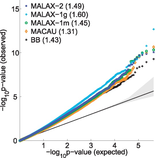
A QQ plot of the P-values obtained by the evaluated methods in the analysis of the baboons data

Next, we examined the effect of adding a second variance component, by comparing the results of MALAX-2 and MACAU. The correlation between the P-values computed by MALAX-2 and by MACAU (Pearson correlation = 0.889, Spearman correlation = 0.835) was substantially lower than between MALAX-1g and MACAU, as expected based on the difference between their underlying models. Additionally, there were several substantial differences between the top ranking P-values computed by MALAX-2 and by MACAU (Fig. 6, Table 1). Namely, 2 of the 10 sites ranked highest by MACAU were ranked substantially lower by MALAX-2, possibly indicating spurious results. Notably, the site ranked highest by MACAU (chr17, locus 8 779 721) obtained a non-significant P-value of 0.15 by MALAX-2. In contrast, the 10 sites ranked highest by MALAX-2 all received P-values < 8 × 10⁻⁵ by MACAU, and were among its 700 top ranking sites. Although these results are suggestive that inclusion of a second variance component can be beneficial, additional in-depth analysis is required to verify the results obtained by the two methods.

Fig. 6.

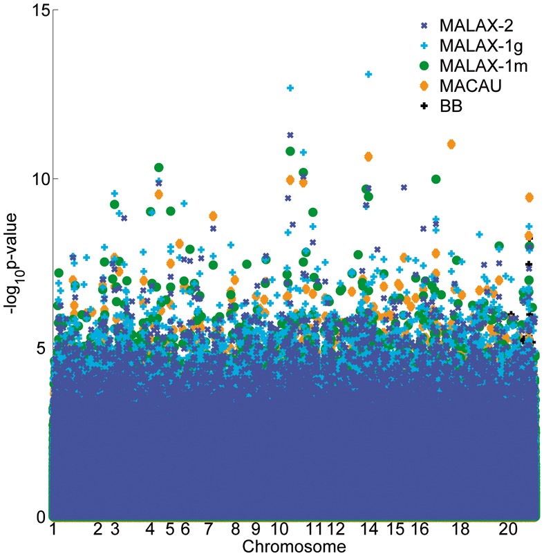
A Manhattan plot of the P-values obtained by the evaluated methods in the analysis of the baboons data. The axis labels for several chromosomes are omitted to improve clarity

Table 1.

The top 10 sites found by MALAX-2 and MACAU in the analysis of the baboons data

MALAX-2						MACAU
rank	chr	pos	P-value	alt. rank	alt. P-value	rank	chr	pos	P-value	alt. rank	alt. P-value
1	10	19 531 653	5.10 × 10–12	3	1.09 × 10–10	1	17	8 779 721	9.57 × 10–12	108 947	1.53E-01
2	10	76 782 787	8.61 × 10–11	4	1.30 × 10–10	2	13	127 550 470	2.23 × 10–11	5	1.92 × 10–10
3	4	43 268 737	1.37 × 10–10	5	2.92 × 10–10	3	10	19 531 653	1.09 × 10–10	1	5.10 × 10–12
4	15	4 962 834	1.81 × 10–10	11	2.18 × 10–8	4	10	76 782 787	1.30 × 10–10	2	8.61 × 10–11
5	13	127 550 470	1.92 × 10–10	2	2.23 × 10–11	5	4	43 268 737	2.92 × 10–10	3	1.37 × 10–10
6	10	13 480 448	3.75 × 10–10	42	2.93 × 10–7	6	20	67 348 840	3.57 × 10–10	14	1.06 × 10–8
7	13	118 109 650	6.02 × 10–10	47	3.62 × 10–7	7	7	19 570 278	1.27 × 10–9	11	2.98 × 10–9
8	3	33 299 965	1.47 × 10–9	115	2.59 × 10–6	8	20	67 035 039	4.88 × 10–9	50	3.13 × 10–7
9	16	48 764 429	2.18 × 10–9	10	1.63 × 10–8	9	5	100 757 817	8.39 × 10–9	8043	2.75 × 10–3
10	10	31 702 787	2.27 × 10–9	696	7.58 × 10–5	10	16	48 764 429	1.63 × 10–8	9	2.18 × 10–9

For each top site, we report its chromosome (chr), position (pos), rank and P-value under the main method and its rank and P-value under the alternative method.

We also evaluated the performance of two recently proposed methods for GLMM approximations (Chen et al., 2016; Jiang et al., 2016), and found that their reported top sites were substantially different from each other and from the top sites reported by MALAX and MACAU, which likely indicates low power on this dataset (results not shown).

Finally, we evaluated the run time of the evaluated methods. The BB model completed the analysis in 4 hours, MALAX-2, MALAX-1g and MALAX-1m completed the analysis in 8.2, 7.45 and 7.77 h, respectively, and MACAU with default parameters competed the analysis in 23.6 h. These results demonstrate that MALAX can reduce the running time required to perform an epigenome-wide analysis by over 50%.

4 Discussion

We presented MALAX, a novel method for association testing for count data, which is especially useful for analysis of data generated by bisulfite-sequencing. MALAX adopts the probabilistic model initially proposed by MACAU, but unlike MACAU, it can be used in the presence of multiple variance components representing diverse sources of confounding. Additionally, MALAX directly approximates the likelihood function via a Laplace approximation, and is thus both conceptually simpler and computationally faster than MACAU, which adopts a Bayesian framework and requires expensive MCMC-based analysis.

Long read-sequencing technologies, such as the Pacific Biosciences and the Oxford Nanopore platforms (Goodwin et al., 2016), may eventually replace bisulfite sequencing for EWAS purposes. However, analysis of methylation data via MALAX will remain useful as long as these technologies cannot probe methylation at a very high coverage at reasonable costs. We further point out that MALAX is a general technique for GLMM approximation. Consequently, MALAX can be readily adapted to other settings with non-normally distributed responses, such as analysis of gene expression data obtained via RNA sequencing (Sun et al., 2016).

In recent years, several methods for GLMM approximations have been proposed in statistical genetics and other domains: GMMAT (Chen et al., 2016) and CARAT (Jiang et al., 2016) are somewhat similar to MALAX but use simpler approximations, which lead to lower statistical power (Supplementary Material). Variational approximation and Expectation Propagation are two methods which approximate the likelihood of GLMMs in a different manner than MALAX (Nickisch and Rasmussen, 2008), but are much slower and do not provide an advantage over MALAX in practice (results not shown). Finally, INLA (Rue et al., 2009), adopts a Bayesian framework similarly to MACAU, but approximates the likelihood analytically similarly to MALAX. Our results indicate that such a Bayesian framework is not required for association testing, but we note that INLA might be useful should one wish to adopt a Bayesian framework without resorting to expensive MCMC computations.

Although MALAX can be over 50% faster than MACAU, both methods have the same computational bottleneck of having to invert or compute determinants of matrices of size n × n, whose computation scales cubically with the sample size under standard implementations. Therefore, both methods cannot currently be used with samples of thousands of individuals. In the future, we intend to investigate the possibility to accelerate MALAX via low rank matrix approximations, using techniques such as the Nyström method (Drineas and Mahoney, 2005), incomplete Cholesky factorization (Fine and Scheinberg, 2001) or Bregman matrix divergence kernel learning (Kulis et al., 2009).

In this work, we evaluated several implementations of MALAX, which are differentiated by using different combinations of variance components. In practice, the use of MALAX requires domain knowledge in order to select the set of variance components that can control for all the sources of confounding in a given dataset, similarly to the use of LMMs in practice.

Finally, the experiments in this paper used the technique of (Zou et al., 2014) to construct a matrix of methylation similarities, which can potentially capture sources of confounding such as cell-type composition. Recently, another technique has been demonstrated to improve control for cell-type composition by first selecting a subset of the methylation sites, and then incorporating the top principal components of the selected sites as covariates (Rahmani et al., 2016). However, both methods suffer from the caveat that there is currently no analytical proof or empirical evidence that they are suitable for the analysis of bisulfite-sequencing data. Specifically, a major difficulty is that computation of methylation similarity matrices and of their principal components is unreliable in the presence of a small number of reads. Adapting one of the above techniques for bisulfite-sequencing data therefore remains a future endeavor.

Funding

This research was partially supported by the Edmond J. Safra Center for Bioinformatics at Tel Aviv University. E.H., and R.S. and E.R. were supported in part by the Israel Science Foundation [Grant 1425/13], E.H. and R.S. by the US Israel Binational Science Foundation grant 2012304, E.R. by Len Blavatnik and the Blavatnik Research Foundation, R.S. by the Colton Family Foundation, and S.R. by the Israeli Science Foundation [grants 1487/12 and 1804/16].

Conflict of Interest: none declared.

References

- Balding D.J., Nichols R.A. (1995) A method for quantifying differentiation between populations at multi-allelic loci and its implications for investigating identity and paternity. Genetica, 96, 3–12. [DOI] [PubMed] [Google Scholar]
- Behnel S. et al. (2011) Cython: the best of both worlds. Comput. Sci. Eng., 13, 31–39. [Google Scholar]
- Bird A. (2007) Perceptions of epigenetics. Nature, 447, 396–398. [DOI] [PubMed] [Google Scholar]
- Byrd R.H. et al. (1995) A limited memory algorithm for bound constrained optimization. SIAM J. Sci. Comput, 16, 1190–1208. [Google Scholar]
- Chen H. et al. (2016) Control for population structure and relatedness for binary traits in genetic association studies via logistic mixed models. Am. J. Hum. Genet., 98, 653–666. [DOI] [PMC free article] [PubMed] [Google Scholar]
- Cohen K.A. et al. (2016) Paradoxical hypersusceptibility of drug-resistant m. tuberculosis to β-lactam antibiotics. EBioMedicine, 9, 170–179. [DOI] [PMC free article] [PubMed] [Google Scholar]
- Cokus S.J. et al. (2008) Shotgun bisulphite sequencing of the Arabidopsis genome reveals DNA methylation patterning. Nature, 452, 215–219. [DOI] [PMC free article] [PubMed] [Google Scholar]
- Devlin B., Roeder K. (1999) Genomic control for association studies. Biometrics, 55, 997–1004. [DOI] [PubMed] [Google Scholar]
- Dolzhenko E., Smith A.D. (2014) Using beta-binomial regression for high-precision differential methylation analysis in multifactor whole-genome bisulfite sequencing experiments. BMC Bioinformatics, 15, 215.. [DOI] [PMC free article] [PubMed] [Google Scholar]
- Drineas P., Mahoney M.W. (2005) On the Nyström method for approximating a gram matrix for improved kernel-based learning. J. Mach. Learn. Res., 6, 2153–2175. [Google Scholar]
- Feng H. et al. (2014) A Bayesian hierarchical model to detect differentially methylated loci from single nucleotide resolution sequencing data. Nucleic Acids Res., 42, e69.. [DOI] [PMC free article] [PubMed] [Google Scholar]
- Fine S., Scheinberg K. (2001) Efficient SVM training using low-rank kernel representations. J. Mach. Learn. Res., 2, 243–264. [Google Scholar]
- Goodwin S. et al. (2016) Coming of age: ten years of next-generation sequencing technologies. Nat. Rev. Genet., 17, 333–351. [DOI] [PMC free article] [PubMed] [Google Scholar]
- Jaffe A.E., Irizarry R.A. (2014) Accounting for cellular heterogeneity is critical in epigenome-wide association studies. Genome Biol., 15, 1.. [DOI] [PMC free article] [PubMed] [Google Scholar]
- Jiang D. et al. (2016) Retrospective binary-trait association test elucidates genetic architecture of Crohn disease. Am. J. Hum. Genet., 98, 243–255. [DOI] [PMC free article] [PubMed] [Google Scholar]
- Jones E. et al. (2001). Scipy: Open source scientific tools for Python. http://www. scipy. org/ (30 December 2016, date last accessed).
- Jones P.A. (2012) Functions of DNA methylation: islands, start sites, gene bodies and beyond. Nat. Rev. Genet., 13, 484–492. [DOI] [PubMed] [Google Scholar]
- Kahaner D. et al. (1989). Numerical Methods and Software, Vol. 1.Englewood Cliffs, Prentice Hall. [Google Scholar]
- Kulis B. et al. (2009) Low-rank kernel learning with Bregman matrix divergences. J. Mach. Learn. Res., 10, 341–376. [Google Scholar]
- Lea A.J. et al. (2015) A flexible, efficient binomial mixed model for identifying differential dna methylation in bisulfite sequencing data. PLoS Genet., 11, e1005650.. [DOI] [PMC free article] [PubMed] [Google Scholar]
- Nickisch H., Rasmussen C.E. (2008) Approximations for binary Gaussian process classification. J. Mach. Learn. Res., 9, 2035–2078. [Google Scholar]
- Powell J.E. et al. (2013) Congruence of additive and non-additive effects on gene expression estimated from pedigree and SNP data. PLoS Genet., 9, e1003502.. [DOI] [PMC free article] [PubMed] [Google Scholar]
- Rahmani E. et al. (2016) Sparse PCA corrects for cell type heterogeneity in epigenome-wide association studies. Nat. Methods, 13, 443–445. [DOI] [PMC free article] [PubMed] [Google Scholar]
- Rasmussen C., Williams C. (2006). Gaussian Processes for Machine Learning. The MIT Press, Cambridge, MA. [Google Scholar]
- Rue H. et al. (2009) Approximate Bayesian inference for latent Gaussian models by using integrated nested Laplace approximations. J. R. Stat. Soc. B, 71, 319–392. [Google Scholar]
- Sun D. et al. (2014) MOABS: model based analysis of bisulfite sequencing data. Genome Biol., 15, R38.. [DOI] [PMC free article] [PubMed] [Google Scholar]
- Sun S. et al. (2016) Differential expression analysis for RNAseq using Poisson mixed models. Nucleic Acids Res., In press. [DOI] [PMC free article] [PubMed] [Google Scholar]
- Weissbrod O. et al. (2015) Accurate liability estimation improves power in ascertained case-control studies. Nat. Methods, 12, 332–334. [DOI] [PubMed] [Google Scholar]
- Widmer C. et al. (2014) Further improvements to linear mixed models for genome-wide association studies. Sci. Rep., 4, 6874.. [DOI] [PMC free article] [PubMed] [Google Scholar]
- Yang J. et al. (2014) Advantages and pitfalls in the application of mixed-model association methods. Nat. Genet., 46, 100–106. [DOI] [PMC free article] [PubMed] [Google Scholar]
- Zou J. et al. (2014) Epigenome-wide association studies without the need for cell-type composition. Nat. Methods, 11, 309–311. [DOI] [PubMed] [Google Scholar]
Associated Data
This section collects any data citations, data availability statements, or supplementary materials included in this article.