

Abstract
Motivation
Experimental techniques for measuring chromatin accessibility are expensive and time consuming, appealing for the development of computational approaches to predict open chromatin regions from DNA sequences. Along this direction, existing methods fall into two classes: one based on handcrafted k-mer features and the other based on convolutional neural networks. Although both categories have shown good performance in specific applications thus far, there still lacks a comprehensive framework to integrate useful k-mer co-occurrence information with recent advances in deep learning.
Results
We fill this gap by addressing the problem of chromatin accessibility prediction with a convolutional Long Short-Term Memory (LSTM) network with k-mer embedding. We first split DNA sequences into k-mers and pre-train k-mer embedding vectors based on the co-occurrence matrix of k-mers by using an unsupervised representation learning approach. We then construct a supervised deep learning architecture comprised of an embedding layer, three convolutional layers and a Bidirectional LSTM (BLSTM) layer for feature learning and classification. We demonstrate that our method gains high-quality fixed-length features from variable-length sequences and consistently outperforms baseline methods. We show that k-mer embedding can effectively enhance model performance by exploring different embedding strategies. We also prove the efficacy of both the convolution and the BLSTM layers by comparing two variations of the network architecture. We confirm the robustness of our model to hyper-parameters by performing sensitivity analysis. We hope our method can eventually reinforce our understanding of employing deep learning in genomic studies and shed light on research regarding mechanisms of chromatin accessibility.
Availability and implementation
The source code can be downloaded from https://github.com/minxueric/ismb2017_lstm.
Supplementary information
Supplementary materials are available at Bioinformatics online.
1 Introduction
In every human cell, genetic and regulatory information is stored in chromatin, where DNA is tightly packed and wrapped around histone proteins. The chromatin structure affects gene expression, protein expression, biological pathway and eventually complex phenotypes. Concretely, some regions of the genome are accessible to transcription factors (TFs), RNA polymerases (RNAPs) and other cellular machines involved in gene expression, while others are compactly wrapped, sequestered and unavailable to most cellular machinery. These two kinds of regions on the genome are known as open regions and closed regions (Wang et al., 2016; Niwa, 2007). Recent high-throughput genome-wide methods invented several biological experiment techniques for measuring the accessibility of chromatin to cellular machines related to gene expression, such as DNase-seq, FAIRE-seq and ATAC-seq. For example, DNase-seq takes advantage of DNase I, a DNA-digestion enzyme, to degrade accessible chromatin while leaving the closed regions largely intact. This assay allows systematic identification of hundreds of thousands of DNase I-hypersensitive sites (DHS) per cell type, and this in turn helps to delineate genomic regulatory compartments (Crawford et al., 2006; Vierstra et al., 2014). Still, biological experiments are expensive and time consuming, making large scale assay impractical and motivating development of computational methods.
In recent years, several sequence-based computational methods have been proposed to identify functional regions, which mainly fall into two classes. One class is the kmer-based methods, where k-mers are defined as oligomers of length k. For example, kmer-SVM provided a support vector machine (SVM) framework for mammalian enhancers discrimination based on k-mer features (Lee et al., 2011). Shortly after kmer-SVM was proposed, gkm-SVM introduced an alternative feature sets named gapped k-mer features, which presented robustness to estimate k-mer frequencies, and consistently improved performance of kmer-SVM (Ghandi et al., 2014). The other class is deep learning-based methods which are mainly established upon convolutional neural networks (CNNs). Indeed, deep learning algorithms are attractive solutions for such sequence modeling problems. DeepBind (Alipanahi et al., 2015) and DeepSEA (Zhou and Troyanskaya, 2015) successfully applied CNNs to modeling the sequence specificity of protein binding with a performance superior to the conventional SVM-based methods. Instead of crafting feature sets like k-mers, CNNs can adaptively capture informative sequence features with aid of convolution operations. Zeng et al. (2016) presented us a systematic exploration of CNN architectures for predicting DNA sequence binding, and showed the benefits of adding more convolutional kernels in learning higher-order sequence features. Moreover, there also exist many other deep learning-based approaches, such as Basset (Kelley et al., 2016) and DeepEnhancer (Min et al., 2016), suggesting us that CNNs have strong power in sequence representation and classification.
Although having been successfully used, both the above two classes of approaches have their own advantages and disadvantages. On one hand, k-mers are an unbiased, general, complete set of sequence features, which can be defined on arbitrary-length sequences. However, k-mers can merely capture local motif patterns without ability to learn long-distance dependencies of DNA sequences. On the other hand, CNNs can detect sequence motifs automatically and yield superior performance in classification tasks. Despite this, one biggest disadvantage for CNNs is that they usually require fixed-length sequences as input, which may limit their application. Besides, almost without exception, current deep learning-based methods simply transform DNA sequences composed of four bases into images with four channels corresponding to A, C, G and T, using one-hot encoding. With such representation, these methods actually execute one-dimensional convolution operations on binary images with only two possible values for each pixel rather than on real continuous-valued images in computer vision field (Krizhevsky et al., 2012), which may impose restrictive effects on their performance.
In fact, it is more natural to regard one DNA sequence as a sentence with four types of characters, namely A, C, G and T, rather than an image, and thus related research work in natural language processing has offered valuable experience for DNA sequence modeling. To address the sentence classification task, Kim (2014) trained CNNs with one layer of convolution on top of word vectors obtained from an unsupervised neural language model. Word vectors, wherein words are projected from a sparse, one-hot encoding onto a lower dimensional vector space via language models such as well-known Skip-gram (Mikolov et al., 2013) and GloVe (Pennington et al., 2014), are essentially semantic features that encode contextual information of words. In this work, the author used word vectors trained by Mikolov et al. (2013) on a corpus of Google News which are publicly available and achieved excellent results on multiple benchmarks, suggesting that the pre-trained vectors are useful feature extractors that can be utilized for various classification tasks. In addition, due to their capability for processing arbitrary-length sequences, the recurrent neural network (RNN) is a natural choice for sentence modeling tasks. Especially, RNNs with Long Short-Term Memory (LSTM) units (Hochreiter and Schmidhuber, 1997) have re-emerged as a popular architecture because of their representational power and effectiveness at capturing long-term dependencies. For instance, Tai et al. (2015) successfully generalized the standard LSTM to tree-structured network topologies and showed their superiority for representing sentence meaning.
With the above consideration, we address the problem of predicting chromatin accessibility from DNA sequence, by proposing an innovative computational approach, namely convolutional long short-term memory networks with k-mer embedding, as shown in Figure 1. We overcome the drawbacks of current DNA sequence modeling approaches in two aspects: (i) we fuse the informative k-mer features into a deep neural network by embedding k-mers into a low dimension vector space; (ii) we are able to handle variable-length DNA sequences as input and capture long-distance dependencies thanks to LSTM units. Specifically, we first cut original DNA sequences with varying lengths into k-mers in a sliding window fashion. Based on the co-occurrence information of k-mers contained in the resulted corpus, we train an unsupervised GloVe model to obtain embedding vectors of all k-mers. In our supervised deep learning architecture, the first embedding layer is designed to turn an original DNA sequence, i.e. a sequence of k-mer indexes, into dense vectors according to the embedding matrix pre-trained by GloVe. The convolutional layers are intended to scan on the sequence of vectors through one-dimensional filtering operations, together with dropout layers and max-pooling layers. The max-pooling layer is followed by a Bidirectional LSTM (BLSTM) layer, which is capable of learning complex high-level grammar-like relationships and handling variable-length input sequences. The last layers are fully-connected dense layers of rectified linear units (ReLU) with dropout to avoid overfitting, and a two-way softmax output layer to generate the final classification probabilities.
Fig. 1.
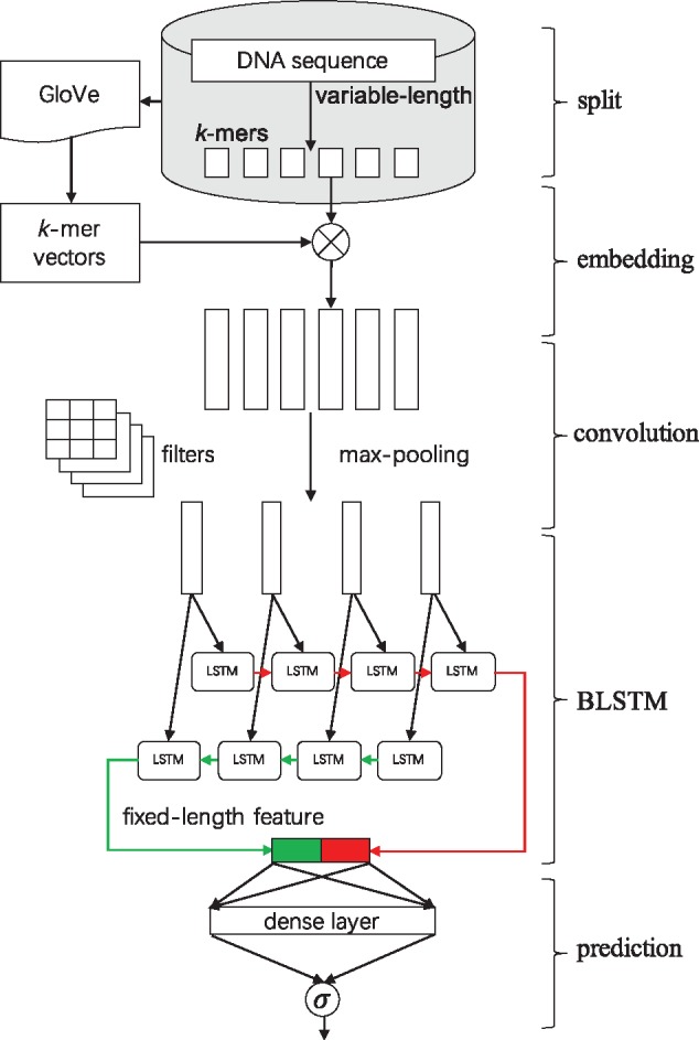
A graphical illustration of our computational framework. We first split every input DNA sequence into k-mers. We use an unsupervised learning method, namely GloVe, to learn the embedding vectors of all the k-mers based on the corpus of k-mer sequences. The embedding layer will embed each k-mer into a vector space based on the GloVe k-mer vectors, which turns the k-mer sequence into a dense real-valued matrix. Then three convolution layers with dropout and max-pooling will scan on the matrix using multiple convolutional filters to detect spatial motifs. The following BLSTM layer contains two LSTMs run in parallel to capture long-range dependencies on the previous output and yield a fixed-length feature representation. The final fully-connected layer and the softmax layer will serve as a classifier to generate probability predictions to be compared with the true target labels via a loss function. For a more detailed description of data shape in each layer, see Supplementary Table S1
To verify the efficacy of our approach, we carry out chromatin accessibility prediction experiments on datasets collected from the Encyclopedia of DNA Elements (ENCODE) project (Consortium et al., 2004). We demonstrate that our framework consistently surpasses other methods on binary classification of DNA sequences. We show that it is beneficial to incorporate the k-mer contextual information into the deep learning framework by learning the low-dimensional real-valued dense embedding vectors. We illustrate that the Bidirectional LSTM units are well-suited for DNA sequence modeling. We expect that our approach could provide insights into general DNA sequence modeling and contribute to understanding of DNA regulatory mechanisms.
2 Materials and methods
In this section, we describe our framework for performing effective deep learning algorithms on DNA sequences data. We begin by constructing the general network architecture that we use. Then we discuss in detail k-mer embedding, which aims to encode the co-occurrence information of k-mers into a low-dimensional vector space by unsupervised learning. In addition, we describe Bidirectional LSTMs, which we applied in order to capture long-range dependencies and form fixed-length feature representation of arbitrary-length DNA sequences.
2.1 General network architecture
Given a DNA sequence of L0 base pairs (bps), we first split it into k-mers using the sliding window approach. We extract all subsequences of length k with stride s, resulting in a k-mer sequence with length , wherein all these k-mers are indexed by positive integers in set . We will investigate how to do feature learning for such sequence data with varying length L, i.e. how to learn a feature map that maps into a vector of features useful for machine learning tasks.
Suppose that we have N variable-length DNA sequences, each with a binary label representing whether it is a chromatin accessible region in a specific cell type. Thus, we have N labeled instances , where . Notice again, length L is varying across samples. Our goal is to learn a function which can be used to assign the label to each instance xi. We use a convolutional long short-term memory network with k-mer embedding as shown in Figure 1. We can decompose the feature learning function into three stages:
| (1) |
The embedding stage computes the co-occurrence statistics of k-mers, and learns to project them into a D-dimensional space . The convolution stage scans on the embedding representation of sequences using a set of one-dimensional convolution filters in order to capture sequence patterns or motifs. The BLSTM stage performs a Bidirectional LSTM network on the input to learn long-term dependencies, and finally yields a fixed-length feature vector in .
Eventually, in the supervised training stage, we treat the binary classification as a logistic regression on the feature representations. The conditional likelihood of yi given xi and model parameters can be written as:
| (2) |
where is the prediction parameters, is the learned fixed-length feature for xi, and is the logistic sigmoid function. We train our deep neural network by minimizing the following loss function:
| (3) |
2.2 k-mer embedding with GloVe
This section explains why and how we embed k-mers into a low-dimensional vector space. As mentioned above, traditional kmer-based methods simply calculate the vector of k-mer frequencies without utilizing the co-occurrence relationship of k-mers. The k-mer feature is an analogy of the ‘Bag-of-Words’ feature (Harris, 1954) widely used in natural language processing and information retrieval, which is an orderless document representation. Meanwhile, the co-occurrence matrix contains global statistical information, which may assist us to construct better feature representations. Here, we apply the popular GloVe (Pennington et al., 2014) model for k-mer embedding, where GloVe stands for ‘Global Vectors’ for word representation based on factorizing a matrix of word co-occurrence statistics. The superiority of GloVe over other methods for learning vector space representations lies in that it combines the advantages of both global matrix factorization and local context window methods.
The statistics of k-mer occurrences are the primary source of information available for learning embedding representations. Let us denote the matrix of kmer-kmer co-occurrence counts by X, whose entry Xij tabulates the number of times that k-mer j occurs in the context window of k-mer i. i, j ∈ [1, V] are two k-mer indexes, where V = 4k is the vocabulary size. According to the GloVe model, the cost function to be minimized is,
| (4) |
where are expected k-mer vectors, are separate context vectors for auxiliary purpose, and are biases. The non-decreasing weighting function f can be parameterized as,
| (5) |
where xmax is a cutoff value and α controls the fractional power scaling which is usually set to 3/4.
As can been seen from Equation (4), the computational complexity depends on the number of nonzero entries in the co-occurrence matrix X. We minimize the cost function in Equation (4) using AdaGrad (Duchi et al., 2011) to obtain our embedding vector representations for all k-mers. Given these vectors, we can fulfill the embedding stage of feature learning by embedding every k-mer into the vector space :
| (6) |
where . Based on the output D × L matrix, we proceed with the convolution stage, which further extracts spatial features using convolutional layers and max-pooling layers.
2.3 Bidirectional LSTM
This section introduces the LSTM unit and explains how a Bidirectional LSTM network can produce a fixed-length output regardless of input sequence lengths. RNNs are able to process input sequences of arbitrary length by means of the recursive application of a transition function on a hidden state vector . At each time step t, the hidden state vector ht is the function of the input vector xt received at time t and its previous hidden state ht–1. Commonly, the RNN transition function is an affine transformation followed by a point-wise nonlinearity such as the hyperbolic tangent function:
| (7) |
Unfortunately, a problem with transition functions of this form is that components of the gradient vector can grow or degrade exponentially over long sequences during training (Hochreiter, 1998; Bengio et al., 1994). Hence, the LSTM architecture (Hochreiter and Schmidhuber, 1997) is designed to remedy this exploding or vanishing gradients problem in RNNs by introducing a memory cell which can choose to retain their memory over arbitrary periods of time and also forget if necessary. While various LSTM variants have been described, here we present the transition equations in Equations (8)–(13) stating the forward recursions for a single LSTM layer.
We define the LSTM unit at each time step t to be a collection of vectors in : an input gate it, a forget gate ft, an output gate ot, an input modulation gate gt, a memory cell ct and a hidden state ht. The entries of the gating vectors it, ft and ot are in [0, 1]. The LSTM transition equations are the following:
| (8) |
| (9) |
| (10) |
| (11) |
| (12) |
| (13) |
where xt denotes the input from the previous layer at the current time step, σ denotes the logistic sigmoid function and denotes element-wise multiplication (Fig. 2).
Fig. 2.
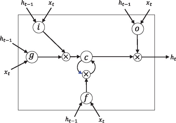
Elaborate description of the LSTM unit. i: input gate, f: forget gate, o: output gate, g: input modulation gate, c: memory cell, h: hidden state. The blue arrowhead refers to ct–1, namely the memory cell at the previous time step. The notations correspond to Equations (8) - (13) such that W(°) denotes weights for xt to the output gate, and U(f) denotes weights for ht–1 to the forget gate, etc. Adapted from Sønderby et al. (2015)
Intuitively, the hidden state vector in an LSTM unit is a gated, partial view of the state of the unit’s internal memory cell. Since the value of the gating variables varies for each vector element, the model can learn the long-range information over multiple time scales. In our application, we only output the hidden state vector of LSTM at the last time step, which remembers the whole sequence information and keeps a fixed-length representation for variable-length input sequences. Besides, a common-used variant of the basic LSTM is the Bidirectional LSTM, which consists of two LSTMs run in parallel: one on the input sequence and the other on the reverse of the input sequence. We concatenate the outputs of two parallel LSTMs to obtain our final feature representation containing both the forward and backward information of a DNA sequence.
3 Results and discussion
To verify our framework, we run a series of classification experiments using datasets collected from the ENCODE project. First, in Section 3.1, we give an introduction to the datasets prepared for classification tasks and some details about model training procedure. Then in Section 3.2, we evaluate our method and compare its performance with gkmSVM and DeepSEA. Next in Section 3.3, we analyze k-mer embedding by probing into the k-mer statistics and visualizing the embedding vectors. Additionally in Section 3.4, we prove the effectiveness of k-mer embedding by exploring different embedding strategies in our network architecture. In Section 3.5 and 3.6, we prove the efficacy of both the convolution and BLSTM stages, by proposing two variant deep learning architectures. Finally in Section 3.7, we perform sensitivity analysis to show the robustness of our model.
3.1 Experiment setup
To benchmark the performance of our deep learning framework, we selected DNase-seq experiments of six typical cell lines, including GM12878, K562, MCF-7, HeLa-S3, H1-hESC and HepG2. GM12878 is a lymphoblastoid cell line produced from the blood of a female donor with northern and western European ancestry by EBV transformation. K562 is an immortalized cell line produced from a female patient with chronic myelogenous leukemia (CML). MCF-7 is a breast cancer cell line isolated in 1970 from a 69-year-old Caucasian woman. HeLa-S3 is an immortalized cell line that was derived from a cervical cancer patient. H1-hESC is a human embryonic stem cell (ESC) line. HepG2 is a cell line derived from a male patient with liver carcinoma.
For each cell type, we downloaded raw sequencing data from website of ENCODE, mapped reads to human reference genome (hg19) using the tool bowtie, and identified chromatin accessible regions (peaks) using the tool HOTSPOT (John et al., 2011). We regarded these variable-length sequences as positive samples, and additionally generated the negative samples by cropping an equal number of sequences randomly from the whole genome with the same length distribution as the positive samples. In this way, we constructed six chromatin accessibility datasets as described in Table 1. Each dataset has 244–504k samples whose lengths present a long-tailed distribution. We then split at random each dataset into strictly non-overlapping training, validation and test sets with proportion 0.85:0.05:0.10. The training set was used to adjust the weights on the neural network. The validation set was used to avoid overfitting. The test set was used for testing the final solution in order to confirm the actual predictive power of the network.
Table 1.
Description of six cell type-specific datasets for chromatin accessibility prediction
| Cell type | Code | Size | l_max | l_min | l_mean | l_median |
|---|---|---|---|---|---|---|
| GM12878 | ENCSR000EMT | 244692 | 11481 | 36 | 610.95 | 381 |
| K562 | ENCSR000EPC | 418624 | 13307 | 36 | 675.21 | 423 |
| MCF-7 | ENCSR000EPH | 503816 | 12041 | 36 | 471.86 | 361 |
| HeLa-S3 | ENCSR000ENO | 264264 | 11557 | 36 | 615.85 | 420 |
| H1-hESC | ENCSR000EMU | 266868 | 7795 | 36 | 430.26 | 320 |
| HepG2 | ENCSR000ENP | 283148 | 14425 | 36 | 652.73 | 406 |
Note: Code denotes the corresponding code in ENCODE project, size denotes the number of sequences the dataset contains, and l_max, l_min, l_mean and l_median denote the maximum, minimum, mean and median value of sequence lengths in bps, respectively. Note that in our datasets we removed regions shorter than 36 bps, so l_min is always 36 bps.
For the unsupervised training of k-mer embedding, we generated the corpus of k-mer sequences by setting k to 6, and the stride s to 2. Consequently, the k-mer vocabulary size is V = 46 = 4096. We used the C implementation of GloVe model published on website https://github.com/stanfordnlp/GloVe, which is multi-thread and ultra-fast, to obtain the k-mer embedding vectors. With regard to hyper-parameters of GloVe, we set the window size to 15 in computing co-occurrence matrix, the vector size, i.e. the embedding dimension to 100, the cutoff value xmax to 30 000 and the maximum number of iterations to 300.
We implemented our supervised deep neural network by Keras (Chollet, 2015) which is a deep learning library for Theano and Tensorflow. We chose Theano as backend of Keras, while the Tensorflow backend also generated very close results through our testing. The high-performance NVIDIA Tesla K80 GPU was used for model training. During training process, we applied the RMSprop algorithm (Tieleman and Hinton, 2012) for the stochastic optimization of the objective loss function, with the initial learning rate set to 0.001, and batch size set to 3000. We also applied the early stopping strategy with the maximum number of iterations set to 60, and it would stop training after 5 epochs of unimproved loss on the validation set.
3.2 Model evaluation
To begin with, we reported accuracy and cross-entropy loss on training, validation and test sets for our method on six different datasets as described in Table 2. The performance on the test set is fairly close to that on the training set, indicating that our method avoided overfitting due to the usage of validation set and early stop strategy. Among the six datasets, we achieved the best prediction on the MCF-7 dataset with 0.8411 accuracy on its test set. With regard to the model efficiency, our model took around 26-41 training epochs until convergence. The training time for each epoch was between 350 and 699s which was roughly proportional to the size of dataset, while the whole training period consumed about 2.5–7.9h.
Table 2.
Training details for our method on each dataset, including accuracy and cross-entropy loss on training, validation and test sets, number of epochs, average training time for each epoch and total training time
| GM12878 | K562 | MCF-7 | HeLa-S3 | H1-hESC | HepG2 | |
|---|---|---|---|---|---|---|
| Train loss | 0.4194 | 0.4161 | 0.3377 | 0.3818 | 0.3800 | 0.4336 |
| Val loss | 0.4346 | 0.4397 | 0.3634 | 0.3976 | 0.3813 | 0.4514 |
| Test loss | 0.4352 | 0.4342 | 0.3595 | 0.4012 | 0.3748 | 0.4440 |
| Train acc | 0.8080 | 0.8105 | 0.8562 | 0.8333 | 0.8302 | 0.8030 |
| Val acc | 0.7940 | 0.7962 | 0.8397 | 0.8203 | 0.8223 | 0.7841 |
| test acc | 0.7947 | 0.7959 | 0.8411 | 0.8180 | 0.8252 | 0.7871 |
| # epochs | 34 | 35 | 41 | 36 | 26 | 33 |
| Time | 350 s | 559 s | 699 s | 374 s | 357 s | 392 s |
| Total | 3.3 h | 5.4 h | 7.9 h | 3.7 h | 2.5 h | 3.5 h |
Next, we compared the performance of our proposed method and several baseline methods, including the gapped k-mer SVM (gkmSVM) (Ghandi et al., 2014), DeepSEA (Zhou and Troyanskaya, 2015). For gkmSVM, we used the source code published on website http://www.beerlab.org/gkmsvm/. For DeepSEA, we implemented it ourselves using Keras. We slightly modified the network structure of DeepSEA to make it suitable for our task. Besides, to directly prove the effectiveness of k-mer embedding, we also propose a new variant network named ‘one hot’, which is mainly comprised of an embedding layer (embedding A, C, G, T using one-hot encoding), three convolutional layers, and a BLSTM layer. For evaluation purpose, we computed two often-used measures, the area under the receiver operating characteristic curve (auROC) and the area under the precision-recall curve (auPRC), on the test set.
We reported the classification performance measured in auROC and auPRC on the six datasets in Table 3. The results of two measures are consistent with each other. As we can see, with the help of k-mer embedding, our method consistently surpasses the other three baseline methods. On average, our method shows an auROC score 3.9% higher than gkmSVM, and 1.4% higher than DeepSEA. On the MCF-7 dataset, our method yields the best performance with auROC of 0.9212 and auPRC of 0.9156. On the K562 dataset, our method obtains the most significant improvement compared to gkmSVM, with auROC increasing by 7.4% and auPRC increasing by 8.1%. Besides, our method always outperforms the one hot method on six datasets, with 0.013 higher auROC score and 0.012 higher auPRC score on average. This observation enlightens us that the straightforward one-hot encoding is perhaps not the optimal strategy for representation of DNA sequences. In contrast, k-mer embedding integrates the contextual information of k-mers and accordingly improves the feature representation. In addition, gkmSVM shows worse performance than DeepSEA except for the H1-hESC dataset, convincing us that deep learning, which can automatically learn feature representation, is more powerful than SVMs with handcrafted k-mer features. To make our results more solid, we additionally carry out 10-fold cross validation experiments on the six datasets, showing that our model significantly outperforms DeepSEA (Supplementary Tables S2–S7). We also run our model several times with different random seeds, showing stability of our model (Supplementary Table S8).
Table 3.
Classification performance for three different methods in chromatin accessibility prediction experiments
| GM12878 | K562 | MCF-7 | HeLa-S3 | H1-hESC | HepG2 | |
|---|---|---|---|---|---|---|
| (a) auROC | ||||||
| gkmSVM | 0.8528 | 0.8203 | 0.8967 | 0.8648 | 0.8983 | 0.8359 |
| DeepSEA | 0.8788 | 0.8629 | 0.9200 | 0.8903 | 0.8827 | 0.8609 |
| One hot | 0.8711 | 0.8634 | 0.9045 | 0.8909 | 0.9081 | 0.8510 |
| our method | 0.8830 | 0.8809 | 0.9212 | 0.9016 | 0.9097 | 0.8722 |
| (b) auPRC | ||||||
| gkmSVM | 0.8442 | 0.8081 | 0.8860 | 0.8627 | 0.8823 | 0.8123 |
| DeepSEA | 0.8758 | 0.8551 | 0.9146 | 0.8888 | 0.8705 | 0.8508 |
| One hot | 0.8679 | 0.8567 | 0.8997 | 0.8900 | 0.8960 | 0.8418 |
| our method | 0.8774 | 0.8732 | 0.9156 | 0.8992 | 0.8968 | 0.8630 |
Note: The top table records auROC values while the bottom one records auPRC values. Best results are shown in bold.
It is also noteworthy that our method gained superiority of running-time owing to GPU usage. For the H1-hESC dataset, our method consumed only 2.5 h as shown in Table 2. Meanwhile gkmSVM allocated with sixteen threads costed 23.8 h before convergence, meaning that our method is nearly 10 times faster than gkmSVM. Thus benefitting by computer hardware, our approach allows researchers to obtain models of high accuracy within a short time.
For the sake of implementation efficiency, we used the common-used zero-padding and truncating strategy in LSTM networks, which is to pad zeros on the right of short sequences and truncate long sequences to a maximum length, and then adopt the standard batch gradient descent (Wilson and Martinez, 2003). Given the length distributions shown in Figure 3, we set the maximum length to 2000 bps in our experiments. To explore the effect of this hyper-parameter, we changed the maximum length in range of 2000, 1500, 1000 and 500 bps, and re-trained our model on the GM12878 dataset. We reported the our model performance with different maximum length in Table 4. We find that when we decrease the maximum length, the auROC and auPRC scores will decrease slightly, except for a fixed length of 500 bps that leads to significant drop in performance, since some input sequences are truncated leading to information loss. We also find that small maximum length will decrease training time remarkably, because the reduction of input dimension directly decreases computational complexity.
Fig. 3.
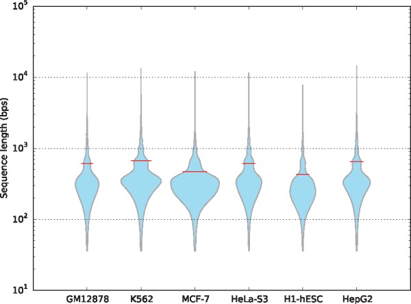
Violin plot for length distribution of DNA sequences in six chromatin accessibility datasets. The width of each violin indicates the dataset size, and the middle red line shows the mean values of sequence lengths
Table 4.
Our model performance on the GM12878 dataset with different maximum length of input sequences
| Length (bps) | auROC | auPRC | Time (s/epoch) | # epochs | Total (h) |
|---|---|---|---|---|---|
| 2000 | 0.8830 | 0.8774 | 350 | 34 | 3.3 |
| 1500 | 0.8793 | 0.8745 | 249 | 32 | 2.2 |
| 1000 | 0.8747 | 0.8682 | 165 | 37 | 1.7 |
| 500 | 0.8528 | 0.8444 | 71 | 30 | 0.6 |
Note: The auROC scores, auPRC scores, average training time for each epoch, number of epochs and total training time are shown.
3.3 Visualization of k-mer embedding
In order to make our model more interpretable, we proceed with a thorough investigation about k-mer embedding in this subsection. The primary specialty discriminating our method from other state-of-the-art deep learning methods in genomic analysis is that we utilize the k-mer embedding vectors trained by GloVe, an unsupervised learning algorithm, as the representation of DNA sequences. Training is based on aggregated global kmer-kmer co-occurrence statistics from a corpus of k-mer sequences, and the resulting representations showcase linear substructures of the k-mer vector space, which benefit subsequent classification tasks.
Take the MCF-7 dataset, for example, we first split its positive samples, i.e. chromatin accessible regions, into k-mer sequences. Thus, taking each k-mer as a word and each k-mer sequence as a sentence, we have a corpus with vocabulary of size V = 4096. We list the top five most frequent k-mers with frequency appended, (aaaaaa, 106157), (tttttt, 104409), (gggagg, 50694), (tgtgtg, 50605) and (cctccc, 50593). The least frequent k-mer is cgtacg occurring only 607 times in total. The overall distribution of k-mer frequencies is depicted in Figure 4a with k-mers ranked by frequency. The symmetric co-occurrence matrix in Figure 4b is normalized via a logarithm function to make patterns more visible. Entries with value <1.0 exist because we applied a distance-weighted function in calculating co-occurrence matrix in practice. There are also 25 823 zero entries displayed in white color which are often found in the right bottom corner.
Fig. 4.
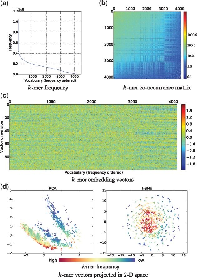
Visualization of k-mer statistics and k-mer embedding vectors in MCF-7 dataset. The top left figure shows the frequency of k-mers. The top right figure illustrates the co-occurrence matrix of k-mers with a log-normalized colormap. The middle figure demonstrates the k-mer vectors produced by GloVe. In the bottom figure, we visualize all the k-mers by projecting their vectors into a plane using PCA and t-SNE
Intuitively, we can see the co-occurrence matrix contains complex patterns and wealthy information of k-mer dependencies on DNA sequences. The 100-dimensional embedding vectors of k-mers learned by GloVe are exhibited in Figure 4c. Statistically, the embedding matrix has a mean value of 0.0016, a maximum value of 1.9883 and a minimum value of –1.9419. We find the weights have a recognizable distribution, i.e. Gaussian distribution with P-value 1.7e-16. Thereby information is relatively decentralized on each dimension which is a good property for feature representation. To visualize the learned k-mer vectors, we show the dimension reduction results using two techniques, Principal Component Analysis (PCA) and t-Distributed Stochastic Neighbor Embedding (t-SNE) (Maaten and Hinton, 2008) in Figure 4d. We put all k-mers as colored circle points in the plot, and we use a continuous colormap to represent their frequency order. Interestingly, although the two methods generate different results, they both declare that k-mers with close frequencies tend to be also adjacent in the embedding vector space.
To further interpret k-mer vectors, we explore how the cosine distance between k-mer vectors is related to the edit distance between k-mers themselves. There are totally 4096 × 4095/2 = 8386560 pairs of k-mers, and we compute the pairwise cosine distance of k-mer vectors and the pairwise edit distance of k-mers. Since there are only six characters in one k-mer, the edit distance has only six possible values, i.e. (1, 2, 3, 4, 5, 6). Thus, we split all the pairs into six groups according to the edit distance. We try to look at each group to see the distribution of their corresponding k-mer vector distances. We summarize the statistics in Table 5 and visualize the distribution of vector distances in Figure 5. In general, we find that the cosine distance between k-mer vectors is monotonically increasing with the edit distance between k-mers. This phenomenon declares the rationality of our k-mer embedding in that the more unlike the two k-mers are, the more faraway they are in the embedding space. For more details, see Supplementary Fig S1, Tables S9 and S10. Besides, we also attempt to investigate the association between the enriched k-mers and the location of these k-mers in chromatin accessible regions, and further the relationship between the enriched k-mers and the DNase-seq signal strength, in Supplementary Fig. S2 and S3. Moreover, we try to find the most specific k-mers corresponding to each cell line, in Supplementary Tables S11 and S12.
Table 5.
k-mer pairs are divided into six groups according to their edit distance
| Edit distance | # pairs | Cosine distance |
|
|---|---|---|---|
| Mean | Std Dev | ||
| 1 | 36 864 | 0.5272 | 0.1466 |
| 2 | 355 494 | 0.8157 | 0.1695 |
| 3 | 1 602 378 | 0.9434 | 0.1414 |
| 4 | 3 272 994 | 1.0006 | 0.1485 |
| 5 | 2 560 482 | 1.0470 | 0.1320 |
| 6 | 558 348 | 1.0822 | 0.1352 |
Note: For each group, we list the number of pairs it contains, and the mean value and the standard deviation of their cosine distances between k-mer vectors.
Fig. 5.
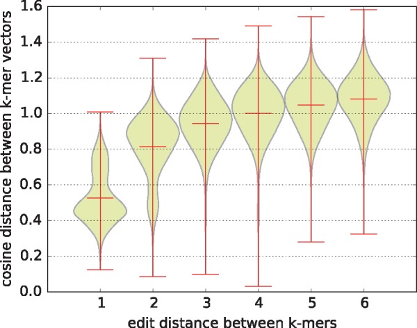
k-mer edit distance versus k-mer vector cosine distance. Each violin describes the distribution of the k-mer vector cosine distances in each group of k-mer pairs, where the intermediate line represents the mean value while the lines on two ends represent extreme values
3.4 Efficacy of k-mer embedding
In our method, the embedding layer is fed with sequences of integers, i.e. k-mer indexes, and then map them to vectors found at the corresponding index in the GloVe embedding matrix. The pre-trained k-mer vectors provide a decent initialization and they will be further fine-tuned during training process. To prove the efficacy of our k-mer embedding, we here put forward two other different embedding strategies. One is to keep the embedding layer fixed during training. The other is that we instead initialize our embedding layer from scratch and learn its weights through training.
We demonstrate auROC scores for the above three embedding strategies on the six datasets in Figure 6. The average auROC scores for ‘-init -train’, ‘-init -notrain’ and ‘-noinit’ strategies are 0.8948, 0.8756 and 0.8726, respectively. We observe that our original strategy brings the best performance as expected. In fact, the combination of unsupervised pre-training and supervised fine-tuning has been proved to be successful in deep learning (Hinton and Salakhutdinov, 2006; Bengio et al., 2007). Moreover, the model reaches a relatively high accuracy just using k-mer embedding vectors without any fine-tuning, consistently outperforming the strategy not using pre-trained vectors. This tells us that, in general, the pre-trained k-mer embedding vectors definitely buy us something of substantial value, and do help improve the model accuracy. For more details, see Supplementary Table S13.
Fig. 6.
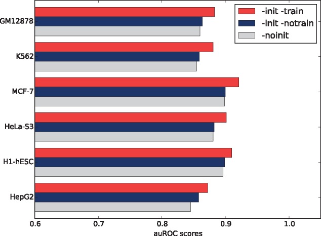
Model performance for different embedding strategies. ‘-init -train’ means that we initialize the embedding layer using the GloVe k-mer vectors, which is adopted in our proposed model. ‘-init -notrain’ means that we initialize the embedding layer using the GloVe k-mer vectors, but prevent the weights from being updated during training. ‘-noinit’ means that we randomly initialize the embedding layer using uniform distribution and allow the neural network to adjust the embedding weights in supervised learning
3.5 Efficacy of convolution
In our experiment, the convolution stage contains three convolutional layers with 100, 100 and 80 one-dimensional filtering kernels of length 10, 8 and 8, each followed by a max-pooling layer with pooling length 4, 2 and 2, respectively. In this subsection, we prove the efficacy of the convolution stage by proposing a variant deep architecture getting rid of the convolutional layers and max-pooling layers from the full model. We directly use the output of the embedding layer as the input of the BLSTM layer instead.
We report the auROC scores and running time of this variant model and compare them against the original full model in Table 6. We discover that removing convolutional layers can obviously injure the auROC score, leading to a 0.0120 decrease on average. This proves the effectiveness of convolutional operations in detecting spatial motifs. With regard to the running time, we find the variant architecture takes almost twice the time to train the network than the full architecture. The reason lies in that the max-pooling layers which down-sample the input representation, play an important role in reducing dimensionality and allowing huge decrease in computation complexity. In view of the above two aspects, we add in the convolution stage in our deep learning framework. For more details, see Supplementary Tables S14 and S15.
Table 6.
auROC scores and running time of two variant deep learning architectures and our original model
| GM12878 | K562 | MCF-7 | HeLa-S3 | H1-hESC | HepG2 | ||
|---|---|---|---|---|---|---|---|
| (a) auROC scores | |||||||
| full | 0.8830 | 0.8809 | 0.9212 | 0.9016 | 0.9097 | 0.8722 | |
| no conv | 0.8746 | 0.8677 | 0.9008 | 0.8878 | 0.9049 | 0.8608 | –0.0120 |
| no lstm | 0.8746 | 0.8741 | 0.9156 | 0.8954 | 0.9087 | 0.8672 | –0.0050 |
| (b) running time for each epoch | |||||||
| full | 350s | 559s | 699s | 374s | 357s | 392s | |
| no conv | 693s | 1173s | 1399s | 739s | 755s | 797s | 465.8s |
| no lstm | 331s | 577s | 690s | 368s | 350s | 384s | –11.8s |
Note: ‘Full’ represents the original architecture comprised of three stages, including a embedding stage, a convolution stage and a BLSTM stage; ‘no conv’ represents the variant architecture removing the convolution stage; ‘no lstm’ represents the variant architecture removing the BLSTM layer, which is substituted by a flatten layer. computes the average difference of auROC scores and running time between the two variants and the full model.
3.6 Efficacy of BLSTM
BLSTM is critical to the processing of variable-length input sequences, and also effective in capturing long-term dependencies. In our method, we have a BLSTM layer with dimension d set to 80. To confirm the efficacy of the BLSTM stage, we construct another variant of our deep learning architecture by retraining the embedding layer and convolutional layers and removing the BLSTM layer. We directly use the flattened output of the convolutional layers instead as our final feature vector for classification.
The auROC scores and the running time for each epoch of this variant architecture and our original full architecture are recorded in Table 6. As expected, the full model always performs better than this variant not using BLSTM, with a 0.0055 improvement in auROC score on average. The running time for the two architectures is quite close to each other, meaning that BLSTM does not increase the computation amount significantly. Note that only the convolutional layers with max-pooling are incapable of dealing with variable length sequences, unless we adopt the aforementioned zero-padding strategy to truncate each sample into the same shape, or we use global pooling (He et al., 2014) instead of max-pooling which extract fixed-dimensional features for temporal data while lose lots of information unfortunately. The results in Table 6a are generated using the former strategy, while the latter one will surely demonstrate even worse performance. Therefore, the BLSTM stage is indispensable in our deep learning architecture for its ability to cope with variable-length sequences and to capture the rich long-term dependencies. For more details, see Supplementary Tables S14–S16.
3.7 Sensitivity analysis
To finish our discussion, we carry out sensitivity analysis to check the robustness of our model. We focus on the following three hyper-parameters: the k-mer length k, the embedding dimension D, and the splitting stride s. Without loss of generality, we use the GM12878 dataset for sensitivity analysis experiments.
According to Figure 7, our model is insensitive to the choice of k and D. Too large k will bring explosive growth of the vocabulary, while too small k may give us too little useful information on the small co-occurrence matrix. We tried three appropriate values of k from 5 to 7, retrained the k-mer embedding vectors, and obtained extremely close performance in classification. Similarly, we also tried four different values of the embedding dimension D, including 50, 100, 150 and 200. A larger D results in more weight parameters to learn in the embedding layer, which will increase the model complexity. Despite this, our model demonstrates quite stable performance, reflecting its ability to avoid overfitting.
Fig. 7.
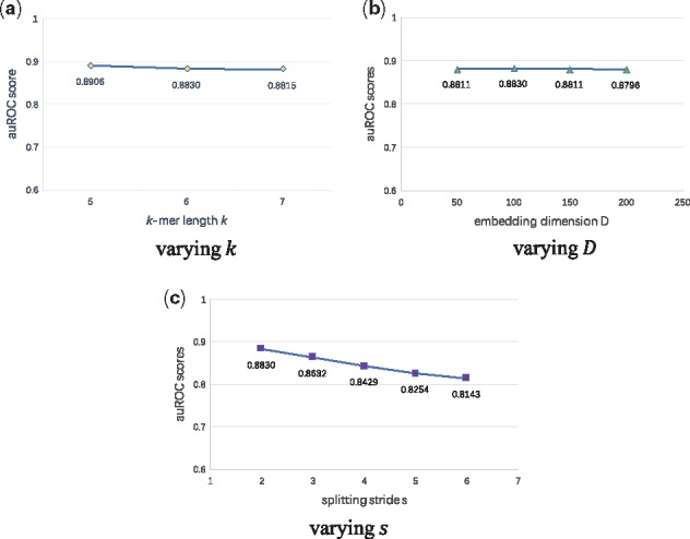
Sensitivity analysis of hyper-parameters k, the embedding dimension D, and the splitting stride s, performed on the GM12878 dataset. The auROC scores on the test set are reported
The splitting stride s will affect the number of k-mers transformed from one DNA sequence by
| (14) |
We find that the auROC score decreases from 0.8830 to 0.8143 when we increase the stride s from 2 to 6. A larger s will decrease the corpus size as Equation (14) said, making part of co-occurrence information lost, and thereby possibly damaging the embedding representation. We do not use the smallest s = 1, since it may cause a too large k-mer corpus and too large overlap between adjacent k-mers, also perhaps harming the embedding algorithm. Considering the above facts, we here recommend a proper splitting stride s = 2 to make full use of k-mer co-occurrence information.
4 Conclusion
In this paper, we propose a convolutional long short-term memory neural network with the pre-trained k-mer embedding vectors to predict chromatin accessible regions from mere sequence information. Our major contributions can be summarized as bellow. First of all, we innovatively introduce an effective embedding representation of input DNA sequences using the unsupervised learning algorithm GloVe in the deep learning framework. Instead of using one-hot encoding, we use the k-mer embedding vectors which have absorbed the statistical information of k-mer co-occurrence relationship and are conducive to following classification tasks, for feature representation. Secondly, we are capable of handling variable-length sequences as input by exploiting the BLSTM network. One big obstacle that hinders the application of CNNs in DNA sequence modeling is the variation in sequence lengths. We utilize the BLSTM networks, not only to make our model appropriate for variable-length input sequences, but also to capture complex long-term dependencies on them. Moreover, we prove our model produces state-of-the-art performance in sequence classification tasks, compared to other baseline methods. We visualize the embedding vectors obtained by GloVe and demonstrate the effectiveness of k-mer embedding. We provide an in-depth understanding of our deep learning architecture, by showing the efficacy of both the convolution and BLSTM stages in feature learning, and showing the robustness of our model to hyper-parameters.
Certainly, our work can possibly be further improved in several aspects. First, the attention mechanism has been successfully introduced to LSTM and improved the performance of neural machine translation (NMT) (Luong et al., 2015). Attention mechanism can selectively focus on parts of sentences during training, and maybe this can be used in our DNA modeling to help detect and visualize the important motifs on sequences. Second, we learn k-mer vectors to embed a DNA sequence into a sequence of dense vectors which is still in variable length, and then extract the fixed-length features through BLSTM. In fact, there exist methods to directly learn distributed representations of sentences and documents, such as Paragraph Vector (Le and Mikolov, 2014), which motivate us to design a more elegant embedding algorithm for vector representation of variable-length sequences. Last but not the least, large-scale experiments of using our model to analyze various kinds of genomics and epigenomics sequencing data is highly encouraged. Eventually, we hope our deep learning method can allow us achieve excellent performance in DNA sequence analysis and help boost our understanding of chromatin accessibility mechanism.
Supplementary Material
Acknowledgement
We thank the anonymous reviewers for their helpful suggestions.
Funding
This research was partially supported by the National Natural Science Foundation of China (Nos. 61573207, 61175002, 71101010, 61673241, 61561146396).
Conflict of Interest: none declared.
References
- Alipanahi B. et al. (2015) Predicting the sequence specificities of DNA-and RNA-binding proteins by deep learning. Nat. Biotechnol., 33(8), 831–838. [DOI] [PubMed] [Google Scholar]
- Bengio Y. et al. (1994) Learning long-term dependencies with gradient descent is difficult. IEEE Trans. Neural Netw., 5, 157–166. [DOI] [PubMed] [Google Scholar]
- Bengio Y. et al. (2007). Greedy layer-wise training of deep networks. In: Advances in Neural Information Processing Systems (NIPS), 19, p.153–160. [Google Scholar]
- Chollet F. (2015). Keras. https://github.com/fchollet/keras.
- Consortium E.P. et al. (2004) The encode (encyclopedia of DNA elements) project. Science, 306, 636–640. [DOI] [PubMed] [Google Scholar]
- Crawford G.E. et al. (2006) Genome-wide mapping of dnase hypersensitive sites using massively parallel signature sequencing (mpss). Genome Res., 16, 123–131. [DOI] [PMC free article] [PubMed] [Google Scholar]
- Duchi J. et al. (2011) Adaptive subgradient methods for online learning and stochastic optimization. J. Mach. Learn. Res., 12, (Jul), 2121–2159. [Google Scholar]
- Ghandi M. et al. (2014) Enhanced regulatory sequence prediction using gapped k-mer features. PLoS Comput. Biol., 10, e1003711. [DOI] [PMC free article] [PubMed] [Google Scholar]
- Harris Z.S. (1954) Distributional structure. Word, 10, 146–162. [Google Scholar]
- He K. et al. (2014). Spatial pyramid pooling in deep convolutional networks for visual recognition. IEEE transactions on pattern analysis and machine intelligence (TPAMI), 37, p.1904–1916. [DOI] [PubMed] [Google Scholar]
- Hinton G.E., Salakhutdinov R.R. (2006) Reducing the dimensionality of data with neural networks. Science, 313, 504–507. [DOI] [PubMed] [Google Scholar]
- Hochreiter S. (1998) The vanishing gradient problem during learning recurrent neural nets and problem solutions. Int. J. Uncertain. Fuzz. Knowledge-Based Syst., 6, 107–116. [Google Scholar]
- Hochreiter S., Schmidhuber J. (1997) Long short-term memory. Neural Comput., 9, 1735–1780. [DOI] [PubMed] [Google Scholar]
- John S. et al. (2011) Chromatin accessibility pre-determines glucocorticoid receptor binding patterns. Nature Genet., 43, 264–268. [DOI] [PMC free article] [PubMed] [Google Scholar]
- Kelley D.R. et al. (2016) Basset: learning the regulatory code of the accessible genome with deep convolutional neural networks. Genome Res., 26(7), 990–999. [DOI] [PMC free article] [PubMed] [Google Scholar]
- Kim Y. (2014). Convolutional neural networks for sentence classification. In: Conference on Empirical Methods on Natural Language Processing (EMNLP), Association for Computational Linguistics (ACL), pp.1746–1751.
- Krizhevsky A. et al. (2012). Imagenet classification with deep convolutional neural networks. In: Platt J.C.et al. (eds) Advances in Neural Information Processing Systems, NIPS. Curran Associates, NY 12571. pp.1097–1105.
- Le Q.V., Mikolov T. (2014). Distributed representations of sentences and documents In: ICML, Vol. 14, p.1188–1196. [Google Scholar]
- Lee D. et al. (2011) Discriminative prediction of mammalian enhancers from dna sequence. Genome Res., 21, 2167–2180. [DOI] [PMC free article] [PubMed] [Google Scholar]
- Luong M.-T. et al. (2015). Effective approaches to attention-based neural machine translation. In: Conference on Empirical Methods on Natural Language Processing (EMNLP), Association for Computational Linguistics (ACL), pp.1412–1421.
- Maaten L. v d., Hinton G. (2008) Visualizing data using t-SNE. J. Mach. Learn. Res., 9, (Nov), 2579–2605. [Google Scholar]
- Mikolov T. et al. (2013). Distributed representations of words and phrases and their compositionality. In: Burges C.J.C.et al. (eds) Advances in Neural Information Processing Systems, NIPS. Curran Associates, NY 12571. pp. 3111–3119.
- Min X. et al. (2016). DeepEnhancer predicting enhancers by convolutional neural networks. In: IEEE International Conference on Bioinformatics and Biomedicine, IEEE, pp. 637–644.
- Niwa H. (2007) Open conformation chromatin and pluripotency. Genes Dev., 21, 2671–2676. [DOI] [PubMed] [Google Scholar]
- Pennington J. et al. (2014). GloVe: global vectors for word representation. In: EMNLP, volume 14, p.1532–43.
- Sønderby S.K. et al. (2015). Convolutional LSTM networks for subcellular localization of proteins. In: International Conference on Algorithms for Computational Biology, p.68–80. Springer International Publishing.
- Tai K.S. et al. (2015). Improved semantic representations from tree-structured long short-term memory networks. In: Annual Meeting of the Association for Computational Linguistics, p.1556.
- Tieleman T., Hinton G. (2012). Lecture 6.5 - rmsprop, COURSERA: Neural networks for machine learning, 4. [Google Scholar]
- Vierstra J. et al. (2014) Coupling transcription factor occupancy to nucleosome architecture with DNase-flash. Nat. Methods, 11, 66–72. [DOI] [PubMed] [Google Scholar]
- Wang Y. et al. (2016) Modeling the causal regulatory network by integrating chromatin accessibility and transcriptome data. Natl. Sci. Rev., 3(2), 240–251. [DOI] [PMC free article] [PubMed] [Google Scholar]
- Wilson D.R., Martinez T.R. (2003) The general inefficiency of batch training for gradient descent learning. Neural Netw., 16, 1429–1451. [DOI] [PubMed] [Google Scholar]
- Zeng H. et al. (2016) Convolutional neural network architectures for predicting DNA-protein binding. Bioinformatics, 32, i121–i127. [DOI] [PMC free article] [PubMed] [Google Scholar]
- Zhou J., Troyanskaya O.G. (2015) Predicting effects of noncoding variants with deep learning-based sequence model. Nat. Methods, 12, 931–934. [DOI] [PMC free article] [PubMed] [Google Scholar]
Associated Data
This section collects any data citations, data availability statements, or supplementary materials included in this article.