Estimation of time-varying growth, uptake and excretion rates from dynamic metabolomics data

Abstract

Motivation

Technological advances in metabolomics have made it possible to monitor the concentration of extracellular metabolites over time. From these data, it is possible to compute the rates of uptake and excretion of the metabolites by a growing cell population, providing precious information on the functioning of intracellular metabolism. The computation of the rate of these exchange reactions, however, is difficult to achieve in practice for a number of reasons, notably noisy measurements, correlations between the concentration profiles of the different extracellular metabolites, and discontinuties in the profiles due to sudden changes in metabolic regime.

Results

We present a method for precisely estimating time-varying uptake and excretion rates from time-series measurements of extracellular metabolite concentrations, specifically addressing all of the above issues. The estimation problem is formulated in a regularized Bayesian framework and solved by a combination of extended Kalman filtering and smoothing. The method is shown to improve upon methods based on spline smoothing of the data. Moreover, when applied to two actual datasets, the method recovers known features of overflow metabolism in Escherichia coli and Lactococcus lactis, and provides evidence for acetate uptake by L. lactis after glucose exhaustion. The results raise interesting perspectives for further work on rate estimation from measurements of intracellular metabolites.

Availability and implementation

The Matlab code for the estimation method is available for download at https://team.inria.fr/ibis/rate-estimation-software/, together with the datasets.

Supplementary information

Supplementary data are available at Bioinformatics online.

1 Introduction

Over the last two decades powerful new technologies for metabolomics enabling the high-throughput quantification of metabolites have emerged. These technologies, usually based on mass spectrometry (MS) or nuclear magnetic resonance (NMR), may be directed with high precision at specific classes of metabolites (targeted approaches) or provide a global scan of the entire metabolome (untargeted approaches) (Patti et al., 2012). Extracellular metabolites, accumulating in or disappearing from the growth medium, are particularly interesting. Their time profiles, while being relatively easy to measure, provide a footprint of intracellular physiology (Kell et al., 2005). In particular, the time-varying concentrations of extracellular metabolites allow the computation of uptake and excretion rates that can be related to intracellular metabolic fluxes by means of flux balance models and metabolic flux analysis (Antoniewicz, 2013; Mo et al., 2009). A variety of applications exploiting the time-course profiles of extracellular metabolites can be found in the literature, increasing our fundamental understanding of the functioning of metabolic networks or informing efforts to reengineer these networks for biotechnological purposes (e.g. Behrends et al. 2009; Morin et al. 2016; Taymaz-Nikerel et al. 2016).

The estimation of time-varying uptake and excretion rates from measurements of extracellular metabolites is a challenging problem for a number of reasons. First, the available data are noisy, even when taking into account continuous progress in metabolomics methods. Second, the time-course profiles of different extracellular metabolites are often strongly correlated. One obvious source of correlation is the proportionality of uptake and excretion rates to the size of the (growing) population of cells consuming or producing the metabolites (Stephanopoulos et al., 1998). Third, the time-course profiles of extracellular metabolites are subject to discontinuities, due to sudden changes in the functioning of metabolism. For instance, in many bacteria catabolite repression leads to the sequential utilization of carbon sources, generally favouring carbon sources that sustain a higher growth rate (Kremling et al., 2015).

Addressing the above issues in a principled manner requires an explicit model relating exchange reactions, concentrations of extracellular metabolites and the size of the cell population. Moreover, we need sound statistical methods for the estimation of the rates from measurements of metabolite concentrations and biomass. Most existing approaches assume the population to be in a state of balanced exponential growth, in which the cell population accumulates at a constant growth rate and in which the rates of exchange reactions are constant. This much simplifies the problem as it reduces rate estimation to a standard linear regression problem (see Murphy and Young 2013 and references therein).

The more general situation in which growth of the microbial population is not balanced has received some attention under the headers of dynamic metabolic flux analysis and dynamic flux balance analysis (Antoniewicz, 2013; Mahadevan et al., 2002). Existing methods for estimating time-varying uptake and excretion rates under these conditions are mostly based on data smoothing using moving averages or splines, followed by explicit computation of the rates by differentiation (Herwig et al., 2001; Llaneras and Picó, 2007; Niklas et al., 2011). Unfortunately, these methods suffer from high sensitivity to noise. This has motivated input estimation methods that do not require differentiation, but fit a parameterized rate function to the concentration data (e.g. Leighty and Antoniewicz 2011). For our purpose, however, these approaches come with a number of drawbacks, in particular the restriction to a specific class of input functions, no exploitation of information shared between correlated concentration profiles, and no (automated) detection of dynamic changes in metabolic regimes.

The aim of this article is to develop a method for precisely estimating time-varying uptake and excretion rates from measurements of extracellular metabolite concentrations, specifically addressing all of the above issues in a comprehensive manner. In order to achieve this, we exploit the fact that the estimation of rates of exchange reactions is an instance of more general input estimation problems that have been extensively studied in control theory and for which powerful solution methods exist (De Nicolao et al., 1997; Pillonetto and Bell, 2007). We follow a regularized Bayesian approach, where the unknown rate profiles are modelled as instances of a random process (Rasmussen and Williams, 2006). In order to capture fast changes in metabolic dynamics, we propose the use of time-varying statistical priors on the unknown rate profiles that are adaptively and automatically determined by suitable data preprocessing, including detection of metabolite depletion for the identification of metabolic regime changes. The resulting estimation problem is then solved by a dynamical smoothing approach, here developed by the combination of extended Kalman filtering and smoothing (Jazwinski, 1970; Kailath et al., 2000). Our approach generalizes upon related work in bioreactor process control, where Kalman filters have been used for on-line estimation of growth rate and reaction rates (Bastin and Dochain, 1990; Venkateswarlu, 2005). Since the data are processed off-line in our case, the additional smoothing step ensures full exploitation of the data and large improvements over standard filtering.

The test of our extended Kalman smoothing (EKS) method to synthetic data with realistic noise levels and a representative number of samples shows excellent performance, superior to results obtained with an approach based on spline smoothing. We also apply our approach to datasets of measured time-varying extracellular metabolite concentrations in Escherichia coli and Lactococcus lactis. The method proves capable of estimating the rates of substrate uptake and by-product excretion with high precision, uncovering notably acetate uptake after glucose depletion in a L. lactis fermentation experiment.

The approach developed in this article provides a comprehensive solution to the three main difficulties of estimating time-varying rates of exchange reactions from extracellular metabolite data—noise, correlated concentration profiles, and discontinuities—using a method with a solid mathematical foundation and wide applicability. An interesting further development would be the generalization of the approach to measurements of intracellular metabolite concentrations, for which increasingly powerful methods operating in real time are becoming available (Link et al., 2015).

2 Problem statement

2.1 Dynamic model of cellular growth in a bioreactor

We consider experiments where the growth of a cellular population in a bioreactor (biomass) and the evolution of the concentration of n extracellular metabolites are monitored over time. Let b(t) denote biomass concentration and c_i(t), with i = 1,…,n, the concentration of the ith metabolite at time t. Biomass and metabolite dynamics are modelled as (Fig. 1)

$$\dot{b}\left(t\right)=\mu \left(t\right)b\left(t\right),$$ (1)

$${\dot{c}}_i\left(t\right)=r_i\left(t\right)b\left(t\right),\hspace{0.17em}\hspace{0.17em}\hspace{0.17em}\hspace{0.17em}\hspace{0.17em}\hspace{0.17em}\hspace{0.17em}\hspace{0.17em}\hspace{0.17em}\hspace{0.17em}\hspace{0.17em}\hspace{0.17em}\hspace{0.17em}\hspace{0.17em}i=1,\dots ,n,$$ (2)

where μ(t) denotes microbial growth rate at time t and r_i(t) is the rate of excretion (if positive) or uptake (if negative) of the ith metabolite per unit of biomass. Equations (1) and (2) form an unstructured model of a growing cell population, ignoring the functioning of internal metabolism but describing its interactions with the environment (Stephanopoulos et al., 1998). The model is based on the assumption that the only causes of changes in concentrations c_i are due to the uptake and excretion rates, thus leaving aside degradation of extracellular metabolites and inflow and outflow of the medium in the bioreactor (Bastin and Dochain, 1990).

Fig. 1.

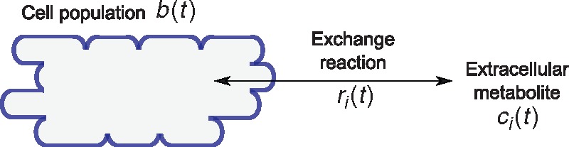
Schematic representation of the model of Equations (1) and (2)

The model of Equations (1) and (2) is a nonlinear system of n + 1 coupled Ordinary Differential Equations (ODEs), with state vector $x={\left[\begin{array}{cccc}b& c_1& \cdots & c_n\end{array}\right]}^T$, input vector $u={\left[\begin{array}{cccc}\mu & r_1& \cdots & r_n\end{array}\right]}^T$ (dependency of the variables on time t is often omitted from notation for brevity), and initial conditions x(t₀) at the starting time t₀ of the experiment. The input profile u(⋅) is assumed to be piecewise continuous, so that the solution of the ODE system is well determined, but not necessarily smooth.

We consider that the different quantities x_i(t), with i = 1,…,n + 1, are measured experimentally at time instants t that may differ across i. Let ${\mathcal{T}}_i$ be a set of measurement times for x_i. For $i=1,\dots ,n+1$, measurements y_i of x_i are modelled as

$$y_i\left(t\right)=x_i\left(t\right)+e_i\left(t\right),\hspace{0.17em}\hspace{0.17em}\hspace{0.17em}\hspace{0.17em}\hspace{0.17em}\hspace{0.17em}\hspace{0.17em}\hspace{0.17em}\hspace{0.17em}\hspace{0.17em}\hspace{0.17em}\hspace{0.17em}\hspace{0.17em}t\in {\mathcal{T}}_i,$$ (3)

where e_i(t) denotes random measurement error with mean zero and standard deviation σ_i(t) > 0. We assume that e_i(t) is statistically independent of $e_{i\prime }(t\prime )$ for any $t\in {\mathcal{T}}_i$ and $t\prime \in {\mathcal{T}}_{i\prime }$ such that $i\ne i\prime$ or $t\ne t\prime$.

In a compact notation, the resulting system is

$$\dot{x}\left(t\right)=f_x\left(x\right(t),u(t\left)\right),\hspace{0.17em}\hspace{0.17em}\hspace{0.17em}\hspace{0.17em}\hspace{0.17em}\hspace{0.17em}\hspace{0.17em}\hspace{0.17em}\hspace{0.17em}\hspace{0.17em}\hspace{0.17em}\hspace{0.17em}\hspace{0.17em}\hspace{0.17em}t\ge t_0,$$ (4)

$$y\left(t\right)=C_x\left(t\right)x\left(t\right)+e\left(t\right),\hspace{0.17em}\hspace{0.17em}\hspace{0.17em}\hspace{0.17em}\hspace{0.17em}\hspace{0.17em}\hspace{0.17em}\hspace{0.17em}\hspace{0.17em}\hspace{0.17em}\hspace{0.17em}\hspace{0.17em}\hspace{0.17em}\hspace{0.17em}t\in \mathcal{T},$$ (5)

with $f_x(x,u)=x_1·u$ and $\mathcal{T}={\mathcal{T}}_1\cup \dots \cup {\mathcal{T}}_{n+1}$. Because the quantities observed at different time instants may not be the same, y(t) is a vector that changes size over time t. At a time t such that $t\in {\mathcal{T}}_{i_1}\cap \dots \cap {\mathcal{T}}_{i_{\ell }}$, with $\{i_1,\dots ,i_{\ell }\}\subseteq \{1,\dots ,n+1\}$ a set with distinct entries, one has that $y={\left[\begin{array}{ccc}{y}_{i_1}& \cdots & y_{i_{\ell }}\end{array}\right]}^T,\hspace{1em}e={\left[\begin{array}{ccc}{e}_{i_1}& \cdots & e_{i_{\ell }}\end{array}\right]}^T$, and $C_x\left(t\right)$ is composed of rows $i_1,\dots ,i_{\ell }$ of an (n+1)-dimensional identity matrix.

2.2 Reconstruction of excretion and uptake rates

Let $\mathcal{Y}=\{{\mathcal{Y}}_1,\dots ,{\mathcal{Y}}_{n+1}\}$ be the set of all measurements ${\mathcal{Y}}_i=\left\{y_i\right(t): t\in {\mathcal{T}}_i\}$, with $i=1,\dots ,n+1$. The challenge we address is the reconstruction of the rate profiles u(t) over a time interval of interest given data $\mathcal{Y}$. The problem is per se ill-posed (Bertero, 1989; De Nicolao et al., 1997), since infinitely many profiles u(t) may perfectly explain the data for a corresponding choice of initial conditions $x\left(t_0\right)$, and the same would hold were $x\left(t_0\right)$ known. In particular, arbitrarily irregular (“wiggly”) profiles u may fit slowly changing measurements of the x_i. To cope with this, methods based on direct data fitting, such as spline interpolation of every observed profile ${\mathcal{Y}}_i$, are often used to compute rate estimates by differentiation of the fits (Herwig et al., 2001; Llaneras and Picó, 2007; Niklas et al., 2011). Unfortunately, these methods may produce unrealistic reconstructions as they inappropriately account for measurement noise and may loose information carried by the coupling of the ODEs through the biomass b.

We therefore recast the problem into the framework of regularized estimation (Wahba, 1990). In this framework, reconstruction is typically expressed as an optimization problem

$$\underset{u\in \mathcal{U}}{\min }\mathcal{Q}\left(u\right)+\lambda \mathcal{R}(u,\mathcal{Y}),$$ (6)

where $\mathcal{U}$ is a convenient class of candidate profiles, $\mathcal{Q}\left(u\right)\ge 0$ is a measure of the regularity of the candidate solution u, and $\mathcal{R}(u,\mathcal{Y})\ge 0$ quantifies the accuracy by which the state profile predicted by (4) in response to u explains the data (for ease of exposition, here $x\left(t_0\right)$ is considered fixed). Parameter $\lambda \ge 0$ trades off regularity of u for accuracy of the data fit. In practice, existing methods consider a parametric class of profiles $\mathcal{U}=\{u_{\theta }: \theta \in \Theta \}$, and (6) is solved in terms of the unknown parameters θ characterizing the input profile (Schelker et al., 2012). While this approach guarantees well-behaved reconstruction of u, the problem remains challenging due to switches in metabolic regime following the depletion of a growth substrate. In practice, this entails abrupt changes in the uptake, excretion, and growth rates u, i.e. extremely fast dynamics that are hard to detect under the necessary regularity assumptions on u, unless explicitly accounted for, e.g. by an ad hoc choice of $\mathcal{U}$ and related definition of $\mathcal{Q}$ and λ.

To address all of these issues, we propose a reconstruction method formulated as a Bayesian regularized estimation problem (Pillonetto and Bell, 2007; Rasmussen and Williams, 2006). The method is based on automatic detection of the switching times and subsequent adaptive choice of the regularity of u. The contrasting objective that this approach is capable to achieve is the reconstruction of slowly-varying rates within a given metabolic regime, together with the detection of abrupt changes in growth, uptake and excretion due to metabolic switches. Moreover, the solution is nonparametric, i.e. both the definition of a parametric class of candidate input profiles $u_{\theta }$ and the corresponding solution of a (typically large) parameter optimization problem are circumvented by means of a dynamic optimization approach. Different from the recent work of Swain et al. (2016) for the estimation of the derivative of an experimental profile, here we address the simultaneous estimation of several unknown rate profiles, with explicit account of nonstationary dynamics, by means of a dynamical approach that is naturally suited to a vast class of nonlinear dynamics.

3 Estimation method

3.1 Bayesian statement of the estimation problem

In a Bayesian setting, regularized estimation starts by placing a statistical prior on the unknown profiles that assigns larger probability to smoother solutions. Consider one entry u_i of $u={\left[\begin{array}{ccc}{u}_1& \cdots & u_{n+1}\end{array}\right]}^T$. One models the unknown profile $u_i\left(t\right)$ as the outcome of a random Gaussian process ${\dot{v}}_i={\gamma }_i{w}_i$ and ${\dot{u}}_i=v_i$, where w_i is standard white Gaussian noise. Intuitively, modelling u_i as this double-integral of white noise implies that u_i is (with probability 1) a continuously differentiable profile, with variability (i.e. probability distribution of its derivative) determined by the magnitude of ${\gamma }_i>0$. In order to account for rates that may undergo faster changes in specific periods of time (switches in metabolic activity), we let γ_i be a function of time, where larger values of ${\gamma }_i\left(t\right)$ around a time point allow for rapid changes of u_i around that time. Taking this model for every $i=1,\dots ,n+1$, and assuming w_i and $w_{i\prime }$ (i.e. u_i and $u_{i\prime }$) to be mutually independent for $i\ne i\prime$, we get the $2·(n+1)$-dimensional linear system of ODEs

$$\dot{\xi }\left(t\right)=A_{\xi }\xi \left(t\right)+B_{\xi }\left(t\right)w\left(t\right),$$ (7)

$$u\left(t\right)=C_{\xi }\xi \left(t\right)$$ (8)

where $\xi ={\left[\begin{array}{ccccc}{v}_1& u_1& \cdots & v_{n+1}& u_{n+1}\end{array}\right]}^T,\hspace{1em}w={\left[\begin{array}{ccc}{w}_1& \cdots & w_{n+1}\end{array}\right]}^T$ is a standard Gaussian noise vector process with uncorrelated entries, and $A_{\xi },\hspace{0.17em}{B}_{\xi }\left(t\right),\hspace{0.17em}{C}_{\xi }$ are equal to

$$\left[\begin{array}{ccccc}0& 0& & & \\ 1& 0& & & \\ & & \ddots & & \\ & & & 0& 0\\ & & & 1& 0\end{array}\right],\hspace{1em}\left[\begin{array}{ccc}{\gamma }_1\left(t\right)& & \\ 0& & \\ & \ddots & \\ & & {\gamma }_{n+1}\left(t\right)\\ & & 0\end{array}\right],\hspace{1em}\left[\begin{array}{ccccc}0& 1& & & \\ & & \ddots & & \\ & & & 0& 1\end{array}\right],$$

in the same order. With this characterization of the unknown rate vector, estimation of u at any time t given data $\mathcal{Y}$ can be formulated as the computation of the conditional expectation $\widehat{u}\left(t\right)=\mathbb{E}\left[u\right(t\left)\right|\mathcal{Y}]$. In practice, the resulting estimate depends on the choice of the γ_i. For a constant γ_i, it can be shown that this approach leads to an estimation problem that is equivalent to a Tikhonov regularization problem in the form of Equation (6), where the role of the regularization factor λ is played by the relative magnitude of the γ_i and the σ_i (De Nicolao et al., 1997; Wahba, 1990). Here, however, we let ${\gamma }_i\left(t\right)$ vary in time so as to distinguish (long) periods with slow rate changes from (short) periods of steep rate transitions. In the following section, we discuss how to (approximately) compute $\widehat{u}\left(t\right)$ for assigned functions ${\gamma }_i\left(t\right)$. We then discuss how a suitable choice of ${\gamma }_i\left(t\right)$ is made by appropriate data preprocessing.

3.2 Solution via nonlinear Kalman smoothing

We start by considering the stochastic differential equation system obtained by the composition of Equations (4)–(5) and (7)–(8). Denoting $z={\left[\begin{array}{cc}{x}^T& {\xi }^T\end{array}\right]}^T$, one gets

$$\dot{z}\left(t\right)=f\left(z\right(t\left)\right)+\omega \left(t\right),\hspace{0.17em}\hspace{0.17em}\hspace{0.17em}\hspace{0.17em}\hspace{0.17em}\hspace{0.17em}\hspace{0.17em}\hspace{0.17em}\hspace{0.17em}\hspace{0.17em}\hspace{0.17em}\hspace{0.17em}\hspace{0.17em}t\ge t_0,$$ (9)

$$y\left(t\right)=C\left(t\right)z\left(t\right)+e\left(t\right),\hspace{0.17em}\hspace{0.17em}\hspace{0.17em}\hspace{0.17em}\hspace{0.17em}\hspace{0.17em}\hspace{0.17em}\hspace{0.17em}\hspace{0.17em}\hspace{0.17em}\hspace{0.17em}\hspace{0.17em}\hspace{0.17em}\hspace{0.17em}\hspace{0.17em}t\in \mathcal{T},$$ (10)

with $f\left(z\right)={\left[\begin{array}{cc}{f}_x(x,C_{\xi }\xi {)}^T& (A_{\xi }\xi {)}^T\end{array}\right]}^T$ and $C\left(t\right)=\left[\begin{array}{cc}{C}_x\left(t\right)& 0_{\ell \times 2·(n+1)}\end{array}\right]$, where $0_{\ell \times 2·(n+1)}$ is a zero matrix of dimensions compatible with $C_x\left(t\right)$. In addition, ω is zero-mean white Gaussian noise with covariance matrix $Q\left(t\right)=B\left(t\right)B{\left(t\right)}^T$, where $B\left(t\right)={\left[\begin{array}{cc}{0}_{(n+1)\times (n+1)}& B_{\xi }{\left(t\right)}^T\end{array}\right]}^T$, while e is a zero-mean random measurement error vector with covariance matrix $R\left(t\right)=\text{diag}({\sigma }_{i_1}^2,\dots ,{\sigma }_{i_{\ell }}^2)$ (recall that $i_1,\dots ,i_{\ell }$ are the entries of x measured at time t).

Together with a priori statistics for the initial state $x\left(t_0\right)$, Equations (9) and (10) describe z as a continuous-time stochastic dynamic system with sampled measurements. By virtue of this, given that u is part of the system state, computation of $\widehat{u}$ can be performed by a dynamical smoothing approach. Here, because the system dynamics are nonlinear, optimal linear Kalman smoothing does not apply, and an approximate solution must be sought. Among many existing approaches (Doucet et al., 2001; Julier and Uhlmann, 2004), we opt for a smoothing approach based on a forward pass in the form of an Extended Kalman Filter (EKF, Jazwinski 1970), followed by a backward correction step in the form of a Bryson-Frazier smoother (Cox 1964; Kailath et al., 2000).

The overall procedure, which we refer to as EKS, works as follows. Let t_j, with $j=0,\dots ,m$, be the elements of $\mathcal{T}$ in increasing order, i.e. the sequence of measurement times. For $j=0,\dots ,m$, let ${\widehat{z}}_j^{-}=\mathbb{E}\left[z\right(t_j\left)\right|y\left(t_0\right),\dots ,y\left(t_{j-1}\right)],\hspace{0.17em}{\widehat{z}}_j=\mathbb{E}[z\left(t_j\right)\left|y\right(t_0),\dots ,y(t_j\left)\right]$ and ${\widehat{z}}_j^{+}=\mathbb{E}\left[z\right(t_j\left)\right|y\left(t_0\right),\dots ,y\left(t_m\right)]$ be the optimal Bayesian one-step prediction, filtered, and smoothed estimate of z at measurement times t_j, in the same order, and let $P_j^{-}$, P_j and $P_j^{+}$ be the corresponding estimation error covariance matrices (Jazwinski, 1970). Recall that z comprises both x and u, i.e. the above quantities provide optimal-prediction, filtered, and smoothed estimates of state x and rates u. Starting from a priori mean ${\widehat{z}}_0^{-}$ and covariance matrix $P_0^{-}$ of the initial state $z\left(t_0\right)$, the following filtering iteration provides approximate computation of ${\widehat{z}}_j^{-}$ and ${\widehat{z}}_j$ for $j=0,1,\dots ,m$:

• Measurement update: Compute

  $$\begin{array}{l}{\widehat{z}}_j={\widehat{z}}_j^{-}+G_j\left(y\right(t_j)-C(t_j\left){\widehat{z}}_j^{-}\right),\\ P_j=(I-G_{j}C(t_j\left)\right)P_j^{-}{(I-G_{j}C(t_j\left)\right)}^T+G_{j}R\left(t_j\right)G_j^T,\end{array}$$

with $G_j=P_j^{-}C{\left(t_j\right)}^T{S}_j^{-1}$ and $S_j=C\left(t_j\right)P_j^{-}C{\left(t_j\right)}^T+R\left(t_j\right)$.

• Prediction: If j < m, compute ${\widehat{z}}_{j+1}^{-}$ and $P_{j+1}^{-}$ as the solutions of

  $$\dot{z}\left(t\right)=f\left(z\right(t\left)\right),\hspace{0.17em}\hspace{0.17em}\hspace{0.17em}\hspace{0.17em}\hspace{0.17em}\hspace{0.17em}\hspace{0.17em}\hspace{0.17em}\hspace{0.17em}\hspace{0.17em}\hspace{0.17em}\hspace{0.17em}z\left(t_j\right)={\widehat{z}}_j,$$ (11)

  $$\dot{P}\left(t\right)=F\left(t\right)P\left(t\right)+P\left(t\right)F{\left(t\right)}^T+Q\left(t\right),\hspace{0.17em}\hspace{0.17em}\hspace{0.17em}\hspace{0.17em}\hspace{0.17em}\hspace{0.17em}\hspace{0.17em}\hspace{0.17em}\hspace{0.17em}P\left(t_j\right)={\widehat{P}}_j$$ (12)

at time $t_{j+1}$, where F(t) is the Jacobian of f(x) evaluated along the solution of Equation (11).

Note that ${\widehat{z}}_m^{+}={\widehat{z}}_m$ and $P_m^{+}=P_m$ by definition. Then, for j < m, a backward iteration provides the computation of the ${\widehat{z}}_j^{+}$ from the results of the filtering pass with the aid of additional recursively computed quantities λ_j and Λ_j. Defining ${\lambda }_m=C{\left(t_m\right)}^T{S}_m^{-1}\left(y\right(t_j)-C(t_j\left){\widehat{z}}_m^{-}\right)$ and ${\Lambda }_m=C{\left(t_m\right)}^T{S}_m^{-1}C\left(t_m\right)$, for $j=m-1,m-2,\dots ,0$:

• Smoothing: Compute

  $${\lambda }_j={\Psi }_j^T{\lambda }_{j+1}+C{\left(t_j\right)}^T{S}_j^{-1}\left(y\right(t_j)-C(t_j\left){\widehat{z}}_j^{-}\right),$$ (13)

  $${\Lambda }_j={\Psi }_j^T{\Lambda }_{j+1}{\Psi }_j+C{\left(t_j\right)}^T{S}_j^{-1}C\left(t_j\right),$$ (14)

  $${\widehat{z}}_j^{+}={\widehat{z}}_j^{-}+P_j^{-}{\lambda }_j,$$ (15)

  $$P_j^{+}=P_j^{-}-P_j^{-}{\Lambda }_j{P}_j^{-},$$ (16)

where ${\Psi }_j={\Phi }_{j+1}-{\Phi }_{j+1}{P}_j^{-}C{\left(t_j\right)}^T{S}_j^{-1}C\left(t_j\right)$ and ${\Phi }_{j+1}$ is the Jacobian of the solution at time $t_{j+1}$ of Equation (11) with respect to the initial condition $z\left(t_j\right)$.

For every j, ${\Phi }_{j+1}$ can be calculated by means of so-called sensitivity equations (Khalil, 2002). Because sensitivity equations and the solution of (12) depend on the solution of (11) in-between time points, in practice, the quantities ${\Phi }_{j+1},\hspace{0.17em}{P}_{j+1}^{-}$ and ${\widehat{z}}_{j+1}^{-}$ are simultaneously calculated (and stored) at every iteration j of the filtering pass by the solution of a single augmented ODE system.

The forward sweep (filtering and prediction) is a standard implementation of the EKF for continuous dynamic systems with sample measurements (Jazwinski, 1970). Yet, the use of a time-varying matrix Q(t) exploiting the time-varying smoothing profiles ${\gamma }_i\left(t\right)$ is nonstandard. The backward sweep (smoothing) described here is a generalization of the method in Cox (1964) to the case of continuous dynamics. For the forward pass, which is critical in ensuring convergence of the approximate solution, EKF showed good performance at very little computational expense. Yet, for especially sparse data sets, a preliminary data interpolation step adapted to the system dynamics is also possible (Supplementary Material S1). Note that the approach is modular, in the sense that more advanced filtering schemes (Doucet et al., 2001; Julier and Uhlmann, 2004) could be used in place of EKF to generate the forward predictions ${\widehat{z}}_j^{-}$ and $P_j^{-}$ used in the smoothing sweep to produce the final estimates ${\widehat{z}}_j^{+}$ and $P_j^{+}$.

The above procedure computes estimates ${\widehat{z}}_j^{+}$ at measurement times. Estimates in-between measurement times are easily obtained by including in $\mathcal{T}$ additional times of interest, and a simple adaptation of the corresponding iterations. The procedure relies on knowledge of the measurement uncertainties σ_i entering matrix R at the various measurement times, of the profiles ${\gamma }_i(·)$ eventually defining the time-varying matrix $Q(·)$, and on given a priori initial state statistics ${\widehat{z}}_0^{-}$ and $P_0^{-}$. While we assume that the σ_i are given, in the following section we discuss how the γ_i (which are typically not known) as well as ${\widehat{z}}_0^{-}$ and $P_0^{-}$ (which are most often partially known) can be determined from suitable data preprocessing. From now on, we will denote the EKS estimates of u and x at a generic time t as $\widehat{u}\left(t\right)$ and $\widehat{x}\left(t\right)$, and the corresponding estimation error covariance matrices as $P_x\left(t\right)$ and $P_u\left(t\right)$. From the latter matrices, credibility (i.e. Bayesian confidence) intervals $X_i^{\alpha }\left(t\right)$ and $U_i^{\alpha }\left(t\right)$ for the estimates of x and u, such that $\mathbb{P}\left[x_i\right(t)\in X_i^{\alpha }(t\left)\right]=\alpha$ and $\mathbb{P}\left[u\right(t)\in U_i^{\alpha }(t\left)\right]=\alpha$, are easily computed. For $\alpha =95\%$, in particular, $X_i^{\alpha }\left(t\right)={\widehat{x}}_i\pm 2·\sqrt{\left(P_x{\left(t\right)}_{i,i}\right)}$ and $U_i^{\alpha }\left(t\right)={\widehat{u}}_i\pm 2·\sqrt{{\left(P_u\right(t\left)\right)}_{i,i}}$.

3.3 Detection of switches and filter tuning

In our approach, the choice of Bayesian priors for the estimated rates is the result of two steps, the determination of smoothing factors for slow and fast dynamics, and the detection of regions where fast dynamics take place. In the interest of affordable computational complexity, these two steps are carried out separately and are finally combined into the definition of the smoothing profiles ${\gamma }_i(·)$.

3.3.1 Calculation of smoothing factors and initial state statistics

Here, we discuss the automated choice of appropriate smoothing profile γ_i and quantities $z_0^{-}$ and $P_0^{-}$ by data preprocessing. This is based on a (not necessarily accurate) pre-estimation of state x_i and rate u_i profiles from data ${\mathcal{Y}}_i$, separately for every i. The same procedure will also be used later on to benchmark the performance of our EKS estimation procedure.

Consider the case i = 1 first. Given data ${\mathcal{Y}}_1$ at times ${\mathcal{T}}_1$, a rough estimate of $b\left(t\right)=x_1\left(t\right)$ over the time period spanned by ${\mathcal{T}}_1$ can be drawn by spline interpolation. We use cubic smoothing splines, so that our interpolation $x_1\left(t\right|\lambda )$ depends on a smoothing parameter λ. In order to ensure an appropriate choice of λ, we resort to the following cross-validation procedure. For a candidate $\lambda >0$, we partition data ${\mathcal{Y}}_1$ into L groups ${\mathcal{Y}}_1^k$ of measurements taken on a set of ${\mathcal{T}}_1^k\subseteq {\mathcal{T}}_1$ subsequent times, with $k=1,\dots ,L$. For every k, we perform smoothed spline interpolation using all data ${\mathcal{Y}}_1^{k\prime }$ with $k\prime \ne k$, and compute ${\mathrm{ϵ}}^k(\lambda )$, the sum of squared residuals of the interpolation at the validation times ${\mathcal{T}}_1^k$. The resulting index $\mathrm{ϵ}(\lambda )={\mathrm{ϵ}}^1(\lambda )+\cdots +{\mathrm{ϵ}}^L(\lambda )$ quantifies the overfitting (lack of predictivity) of the spline interpolations (the larger the $\mathrm{ϵ}(\lambda )$, the worse the interpolation). We choose the value of λ that optimizes $\mathrm{ϵ}(\lambda )$ by numerical minimization. By this optimized smoothing parameter, say ${\tilde{\lambda }}_1$, we finally obtain the optimized smoothing interpolation ${\tilde{x}}_1\left(t\right)=x_1\left(t\right|{\tilde{\lambda }}_1)$. Pre-estimates of the rate profile u₁(t) are then obtained by means of Equation (1), i.e. ${\tilde{u}}_1\left(t\right)=\left(d{\tilde{x}}_1\right(t)/dt)/\left({\tilde{x}}_1\right(t\left)\right)$.

Because of the homogeneity of the smoothing strength over the whole time span, it is expected that estimates of state and rate profiles of appropriate regularity are obtained at all times except at the few rapid transitions from one regime to another, where oversmoothing occurs. By this, ${\tilde{u}}_1\left(t\right)$ provides us with the necessary information on how to choose the smoothing profile ${\gamma }_1\left(t\right)$. Concretely, this is obtained by the following method of general applicability. Recall that, for EKS purposes, u₁ is modelled as a twice-integrated white noise process. For a constant γ₁ over the time interval $[t,t+\tau )$, the increment $u_1(t+\tau )-u_1\left(t\right)$ has mean zero and standard deviation equal to ${\gamma }_1·{\tau }^{3/2}/\sqrt{3}$. Because this standard deviation defines the regularity of ${\tilde{u}}_1$, and because the corresponding ${\tilde{u}}_1(t+\tau )-{\tilde{u}}_1\left(t\right)$ are expected to be of the right order in-between metabolic switches, an appropriate choice of ${\gamma }_1\left(t\right)$ within these periods is such that the standard deviation of $u_1(t+\tau )-u_1\left(t\right)$ equals the average value, say Δ, of $\left|{\tilde{u}}_1\right(t+\tau )-{\tilde{u}}_1(t\left)\right|$ over a grid of times t with sampling period τ. Upon computation of Δ from ${\tilde{u}}_1$, this leads to the definition ${\gamma }_1\left(t\right)={\gamma }_1^{°}$, with ${\gamma }_1^{°}=\Delta /({\tau }^{3/2}/\sqrt{3})$, for all times t in-between switches. Finally, in order to capture proportionally faster dynamics, within periods of fast metabolic changes the smoothing factor is set to ${\gamma }_1\left(t\right)={\gamma }_1^{\infty }$, with ${\gamma }_1^{\infty }={10}^3{\gamma }_1^{°}$.

For $i\ne 1$, a nearly identical procedure is followed. For every i, a cross-validated spline interpolation is operated on data ${\mathcal{Y}}_i$, obtaining an optimized estimate ${\tilde{x}}_i\left(t\right)$ (with its own parameter ${\tilde{\lambda }}_i$). Then, using the previous biomass data interpolation ${\tilde{x}}_1\left(t\right)$, rate pre-estimates are obtained with Equation (2) as ${\tilde{u}}_i\left(t\right)=\left(d{\tilde{x}}_i\right(t)/dt)/\left({\tilde{x}}_1\right(t\left)\right)$. Finally, ${\gamma }_i^{°}$ and ${\gamma }_i^{\infty }$ are set as a function of ${\tilde{u}}_i$ as described above.

Pre-estimates ${\tilde{x}}_i$ and ${\tilde{u}}_i$, with $i=1,\dots ,n+1$, also allow us to fix the initial state statistics ${\widehat{z}}_0^{-}$ and $P_0^{-}$. More precisely, entries of ${\widehat{z}}_0^{-}$ corresponding to x_i (resp. to u_i) are set equal to the initial value of ${\tilde{x}}_i$ (resp. of ${\tilde{u}}_i$), whereas all other entries are set to 0. From this, $P_0^{-}$ is set to be a diagonal matrix with diagonal entries defined elementwise by $\min \{{\left({\widehat{z}}_0^{-}\right)}^2,D\}$, with D big enough. This ensures that priors are sufficiently weak, in order to favour convergence of the EKS without constraining a priori the resulting estimates.

3.3.2 Detection of switches and definition of the smoothing profiles

Switching times are automatically detected by direct processing of the measurements. We exploit the fact that concentrations c_i of some metabolites dropping to zero are typically associated with changes of the metabolic regime. In accordance with this, for every i, a time $t_j\in {\mathcal{T}}_i$ is declared a switching time if $y_i\left(t_j\right)\le 2·{\sigma }_i\left(t\right)$ and the observations $y_i\left(t_{j-1}\right),y_i\left(t_{j-2}\right),\dots ,y_i\left(t_{j-J}\right)$ are above the same threshold.

If a switch at time t_j is detected, the time period where rate changes are expected to be fast is set to $[t_{j-1},t_j]$. Over this switching period, because a drop of c_i can induce sudden rate changes in all metabolites, ${\gamma }_{i\prime }\left(t\right)$ is set to ${\gamma }_{i\prime }^{\infty }$ for $i\prime =1,\dots ,n+1$. Note that the resulting smoothing profiles constitute Bayesian priors that drive the estimation procedure toward estimates with regularity properties of the right order. The actual degree of smoothness and steepness of estimates at sudden metabolic changes is then inherently adjusted by the EKS procedure.

Note that failure to detect a metabolic switch, e.g. due to lack of measurements for critical metabolites, will not spoil the estimation procedure overall, but will return rate estimates that vary at a slow pace at metabolic changes, prompting for either a manual definition of switch times, or a more appropriate experiment design.

3.4 Implementation

The estimation method described in the previous section, comprising data-driven tuning of the EKS and the EKS itself, has been implemented in Matlab. The software takes as input data ${\mathcal{Y}}_1,\dots ,{\mathcal{Y}}_{n+1}$, measurement times ${\mathcal{T}}_1,\dots ,{\mathcal{T}}_{n+1}$, error levels ${\sigma }_1,\dots ,{\sigma }_{n+1}$, and performs tuning as well as estimation in a completely automated fashion. It returns full state (i.e. biomass, concentration and rate) estimated profiles and estimation error covariances, as well as the estimation settings (notably smoothing factor and switch times). Custom settings (for instance, modifications of the output settings) may be specified as well. A more detailed description of the software and its usage is provided in Supplementary Material Section S6.

4 Validation on simulated data

In order to validate the estimation method of Section 3, we now discuss its application to simulated data, so as to compare the estimated reaction rates with the actual reaction rates used for generating the data. As a concrete example, we will consider the phenomenon of overflow metabolism and diauxic growth. Overflow metabolism is a recurrent phenomenon in microorganisms occurring in situations where a primary growth substrate is available in excess and inefficiently used by the cells, in the sense that secondary substrates are secreted during growth on the primary substrate. Once the primary substrate has been depleted, growth continues on the second substrate, often at a lower rate (Kremling et al., 2015; Paczia et al., 2012). A prototypical example of overflow metabolism leading to diauxic growth is aerobic growth of E. coli in minimal medium with glucose, leading to an overflow of acetate that is utilized after glucose exhaustion, giving rise to a so-called acetate switch (Enjalbert et al., 2013; Wolfe, 2005). The simulated experiment in this section is much similar to the actual experiments considered in the following section.

The dynamics of the growing microbial population in the bioreactor and of the extracellular metabolite concentrations, the primary and secondary substrates, are described by Equations (1) and (2) with n = 2. The simulated rates are piecewise constant functions of environmental substrate concentrations. Starting from $\overline{b}=b\left(0\right)>0,\hspace{0.17em}{\overline{c}}_1=c_1\left(0\right)>0$ and ${\overline{c}}_2=c_2\left(0\right)\ge 0$, the primary substrate rate $r_1\left(t\right)$ takes value ${\overline{r}}_1<0$ (uptake) until time t = T₁ where $c_1\left(t\right)$ hits 0, and zero afterwards. The secondary substrate rate $r_2\left(t\right)$ takes value ${\overline{r}}_2>0$ (excretion) until time T₁, then it switches to ${\underset{¯}{r}}_2<0$ (uptake) until time t = T₂ where $c_2\left(t\right)$ hits 0, and zero afterwards. Biomass growth rate takes value $\overline{\mu }>0$ until time T₁ (growth on first substrate), then switches to $\underset{¯}{\mu }$, with $\overline{\mu }>\underset{¯}{\mu }>0$ until time T₂ (growth on second substrate), and to 0 afterwards (growth arrest). We simulated measurements taken at times ${\mathcal{T}}_1=\{t_j=j·T, j=0,\dots ,3m\}$ for biomass, and at sparser times ${\mathcal{T}}_{i+1}=\{t_j=j·3T, j=0,\dots ,m\}$, for the primary and secondary substrates. Random measurement error is added in accordance with Equation (3) with time-homogeneous standard deviations σ_b, ${\sigma }_{c_1},\hspace{0.17em}{\sigma }_{c_2}$. The simulated data are shown in Figure 2a and also separately in Supplementary Material Section 2.1.

Fig. 2.

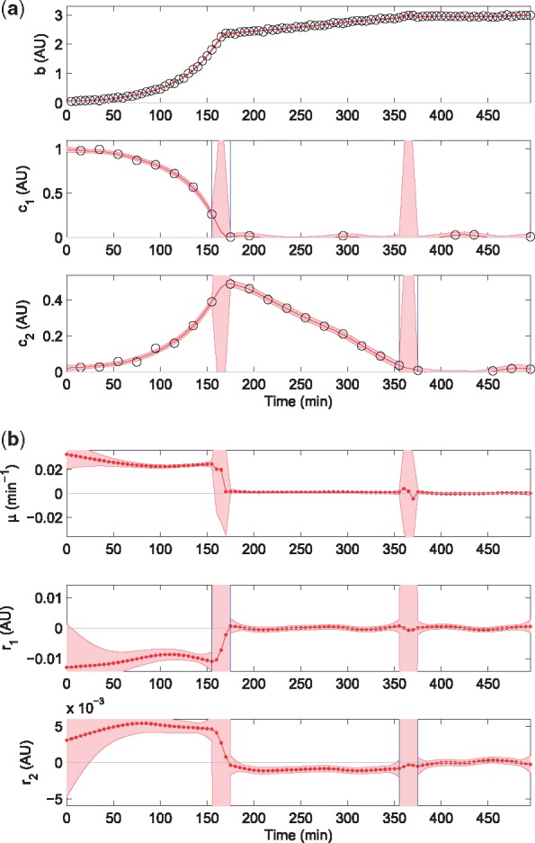
Estimation of exchange rates by applying the EKS method to a dataset obtained by simulating a diauxic growth experiment with overflow metabolism. Simulation parameters are reported in Supplementary Material Section S2.1, showing the simulated data and their confidence intervals. (a) Simulated data (circles), detected switching times (in-between vertical blue lines) when a substrate concentration drops to 0, and EKS estimates of biomass and concentration profiles with their 95% credibility intervals (red curves and bands, respectively). (b) EKS rate estimates from the fully automated procedure with 95% credibility intervals (red curves and bands, respectively)

Figure 2a and b shows the detected depletion of substrates and the EKS estimates of x and u obtained with fully automated filter tuning. Detection of switches at times T₁ (depletion of the primary substrate) and T₂ (depletion of the secondary substrate) is visibly correct in panel (b), and in absence of further information, potentially fast rate changes are authorized in the time interval between the last measurement above and the first below the switching threshold. This gives rise to the rate estimates $\widehat{u}$ displayed in Figure 2b, with a smooth, slowly-varying profile except within the switching periods, where transitions are steep as expected.

The same rate estimates are also reported in Figure 3b, where they are compared with the actual simulated rates and with the rate estimates $\tilde{u}$ found by the smoothing spline method of Section 3.3.1. That EKS estimates $\widehat{u}$ outperform estimates $\tilde{u}$ obtained via spline smoothing is apparent. It is worth remarking how the EKS tuning based on $\tilde{u}$, which operates on the regularity of $\widehat{u}$, does not spoil the EKS estimates themselves (no direct relationship between $\widehat{u}$ and $\tilde{u}$). Yet, rate estimates over constant regimes show residual fluctuations, presumably due to a slight overestimation of the ${\gamma }_i^{°}$ by the automated tuning step. At the same time, estimated rate transitions are still not as abrupt as in the simulations, and the associated credibility intervals are large. This is primarily due to the sparsity of the metabolite measurements, causing the estimated transitions to spread over a somewhat longer period of time. In Figure 3b, small manual adjustments of the settings returned by the procedure yield even better results, with sharp changes closely resembling the actual discontinuous regime changes. It is important to note that these adjustments are driven in a rather intuitive manner by the qualitative analysis of the fully automated estimation results, i.e. they can be operated by a user facing the analysis of experimental data.

Fig. 3.

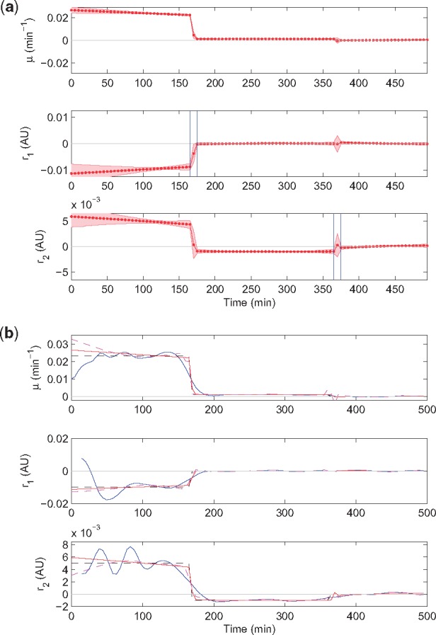
Comparison of the results obtained with different rate estimation methods applied to the data set of Figure 2. (a) EKS rate estimates and their 95% credibility intervals obtained after manual adjustment of the automatically determined switching periods and smoothing factors (red curves and bands, respectively). The adjustments concern a decrease of the length of the transition period to 10 min and a decrease of the smoothing factors $({\gamma }_1^{°},{\gamma }_2^{°},{\gamma }_3^{°})=(1.80,1.87,1.12)\times {10}^{-5}$ to a uniform value of 10^–6 for all i, with ratios ${\gamma }_i^{\infty }/{\gamma }_i^{°}$ unchanged. (b) Comparison of the true rates (dashed black curves) with estimated rates obtained by the spline smoothing method (solid blue curves), by the fully automated EKS method (same as in Fig. 2b; dashed magenta curves), and by a posteriori manual adjustment of the automatic EKS settings (solid red line)

In summary, estimation results for a realistic (noisy) simulated dataset of a diauxic shift experiment show excellent performance of the automated method and significant improvements relative to a reference approach. Basic manual refinements of the data-driven EKS tuning allow the results to be even further improved. Comparison of estimation results with those obtained with EKF (the forward pass of the EKS), which is another approach that has been considered in the literature, also witnesses striking improvements (see Supplementary Fig. S2). The above results are confirmed by an additional simulation example of fed-batch cultivation in Supplementary Material Section S2.2.

5 Applications of rate estimation

5.1 Diauxic growth in E. coli

The first application of the method to a real dataset concerns time-series measurements of glucose, acetate and biomass during aerobic growth of E. coli in minimal medium with glucose and acetate (Morin et al., 2016). The acetate has accumulated in the medium as a by-product of growth on glucose at a rate exceeding the oxydizing capacity of central metabolism. The bacteria were cultivated in a bioreactor in batch mode and samples were taken every 10–30 min over a period of about 6 h, covering rapid exponential growth on glucose, glucose depletion and continued slow growth on acetate. The samples were analysed by high-performance liquid chromatography (HPLC) to quantify the concentrations of extracellular metabolites in the medium (Morin et al., 2016). The resulting measurements for one replicate are shown in Figure 4b and in Supplementary Material Section S2.3.

Fig. 4.

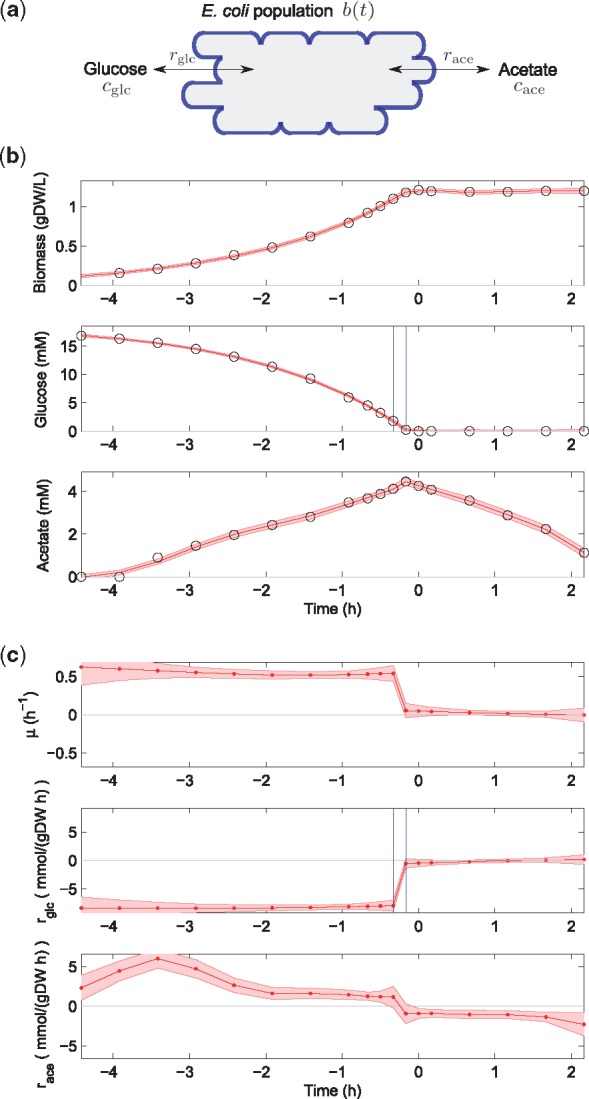
Diauxic growth on glucose and acetate of E. coli. (a) Model scheme defining variables and rates. (b) Data (circles) from Morin et al. (2016) and EKS estimates with credibility intervals (solid curve and shaded band) of biomass and concentration profiles. (c) EKS rate estimates and credibility intervals (red curve and shaded band) obtained with the fully automated procedure described in Section 3. The smoothing parameters found for biomass, glucose and acetate, ${\gamma }_{\mathrm{b}}^{°}=0.675,\hspace{0.17em}{\gamma }_{\text{glc}}^{°}=5.5842$ and ${\gamma }_{\text{ace}}^{°}=8.4025$, were adjusted by a factor of ${10}^{-1},\hspace{0.17em}{10}^{-1}$ and 2^–1, respectively. For a comparison of the EKS estimates with the smoothing spline estimates, see Supplementary Material Section S2.2

The challenge for the analysis of this dataset is to correctly estimate the rapid changes of the uptake and secretion rates around the time of glucose depletion at 0 h, while at the same time provide a stable value for the rates during balanced growth on either glucose (before the switching time) or acetate (after the switching time). The algorithm described in Section 3.2 was run for the three variables biomass (b), glucose concentration ($c_{\text{glc}}$), and acetate concentration ($c_{\text{ace}}$), after a first preprocessing round in which appropriate smoothing profiles and a priori initial state statistics were obtained by spline smoothing and generalized cross validation (Section 3.3). The EKS estimates for the rates are shown in Figure 4c.

The most striking conclusion drawn from the estimation results is the capability of the algorithm to precisely capture the sharp drop in growth rate when the glucose concentration falls to 0, accompanied by an equally abrupt arrest of glucose uptake and switch from acetate excretion to acetate uptake. In contrast, the spline smoothing estimates do not capture this abrupt regime change and, moreover, lead to unstable estimates of the steady-state exchange rates and growth rate, visible as oscillations around the steady-state values (Supplementary Fig. S6).

The importance of the precision of rate estimation can be illustrated by testing the consistency of the results with the reaction stoichiometry of intracellular metabolism, using a flux balance model of E. coli (Feist et al., 2007). In particular, we performed a metabolic flux analysis in the manner of Morin et al. (2016) just before the acetate switch, where the smoothing spline and EKS estimates are most different, and compared estimates for 15 fluxes in central carbon metabolism obtained by flux variability analysis. Interestingly, the smoothing spline estimates yield flux distributions that are much less precise and non-intuitive (Supplementary Material Section S4). For example, the partitioning of the incoming flux of glucose over the glycolysis, pentose-phosphate, and glycogenolysis pathways is not appropriately accounted for, since every pathway can be preferentially used in some optimal solution. In reality, the major part of the incoming glucose flux enters glycolysis (Morin et al., 2016), as observed when using the EKS estimates for metabolic flux analysis (Supplementary Material Section S4).

We found a remarkable consistency between the predicted intracellular fluxes with the EKS estimates, when cells are in quasi steady-state growth two hours before glucose exhaustion, with measured fluxes in a continuous culture of E. coli on glucose (see Supplementary Fig. S10).

5.2 Production of lactic acid by L. lactis

When growing on glucose, lactose or other sugars, the energy metabolism of L. lactis leads to the excretion of large amounts of lactic acid. In addition to being a catalyst for the production of butter milk and cheese, the accumulation of lactic acid in the medium inhibits the growth of microorganisms, including food-borne pathogens. This has motivated interest in L. lactis for the purpose of food conservation (Even et al., 2002). The second application of our rate estimation method concerns a study of the effect of lactic acid overflow on L. lactis growth and the consequences of a glucose pulse on lactic acid production. The bacteria were cultivated in fed-batch in a fermenter and 30 samples were taken over 3 days and analysed by means of HPLC to quantify glucose, lactic acid and acetate concentrations in the medium (see Supplementary Material Section S3 for the experimental protocol). The resulting measurements are shown in Figure 5b and in Supplementary Material Section S2.4.

Fig. 5.

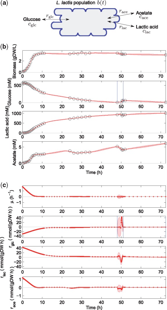
Lactic acid production by L. lactis. (a) Model scheme defining variables and rates. (b) Data (circles) and EKS estimates with credibility intervals (solid red curve and shaded band) of biomass and concentration profiles. The detected switching time lies between the two blue vertical lines. (c) EKS rate estimates and credibility intervals (red curve and shaded band) obtained with the fully automated procedure described in Section 3. The smoothing parameters used for biomass, glucose, lactic acid and acetate are ${\gamma }_{\mathrm{b}}^{°}=0.01,\hspace{0.17em}{\gamma }_{\text{glc}}^{°}=0.1,\hspace{0.17em}{\gamma }_{\text{lac}}^{°}=0.1$ and ${\gamma }_{\text{ace}}^{°}=0.01$, respectively. Factors ${\gamma }_i^{\infty }={10}^3{\gamma }_i^{°}$, as per default settings, except for ${\gamma }_{\text{glc}}^{\infty }={10}^4{\gamma }_{\text{glc}}^{°}$, to cope with glucose addition

The interest of the dataset is (1) to quantify the effect of the lactic acid produced by L. lactis on the growth rate of the cell population and (2) to account for rapid changes in the rates of acetate and lactic acid accumulation following the depletion of glucose just before 50 h and the supply of a glucose pulse shortly afterwards (Fig. 5b). The detection of glucose exhaustion is similar to the previous application, but the addition of a pulse of glucose does not strictly fall within the modeling framework of Equations (1) and (2), which assumes that changes in extracellular metabolite concentrations are only due to uptake and excretion of the metabolites by the growing cell population (and not by external inflow into the bioreactor). While the models can be straightforwardly generalized to cover this case explicitly (see Supplementary Material Section S5), we here sidestep the problem by lumping the rates of glucose uptake and inflow into a single apparent rate for glucose accumulation. The estimation results are summarized in Figure 5c.

A first conclusion that can be drawn from inspecting the estimated rates is that, due to the growth-inhibitory effect of lactic acid accumulation, a state of balanced, non-zero growth is never reached in the first 10 h of the experiment. This problem, well-known in L. lactis cultivation experiments, demonstrates the importance of being able to compute a time-varying growth rate profile rather than report a single value at an arbitrary point along the growth curve. Second, the depletion of glucose just before 50 h is adequately captured by the method, as well as the subsequent uptake of acetate, visible in the negative value of the estimated rate following glucose depletion. This observation, reminescent of diauxic growth in the previous example, is interesting but currently not well understood. Just after the glucose pulse at 50.5 h, the acetate excretion rate becomes slightly positive again, meaning that the bacteria convert the added glucose into lactic acid and acetate, in the absence of biomass accumulation since the growth rate does not noticeably change. This example demonstrates the capability of the method to capture subtle dynamic changes in uptake and excretion rates from concentration profiles of extracellular metabolites.

6 Discussion

Dynamic estimation problems have become ubiquitous in the era of high-throughput data generation in biology. In the study of gene expression, for example, time-series measurements of the fluorescence signals emitted by reporter proteins contain information on time-varying promoter activities (Zulkower et al., 2015), while time-series measurements of signal transduction outputs allow the reconstruction of time-varying inputs, like pathway activation by growth hormones (Schelker et al., 2012). The measurement of extracellular metabolites has become simpler to achieve through ongoing advances in the field of metabolomics and they provide precious information on intracellular metabolism (Kell et al., 2005). These data are often underexploited though, in the sense that in many studies the time-varying rates of substrate uptake and by-product secretion are not computed. Changes in these rates, however, reveal changes in cellular metabolism and may thus be instrumental in systems biology for better understanding the response of cells to external perturbations and in biotechnology for dynamically adapting process conditions.

One of the reasons that time-series measurements of extracellular metabolites are not fully exploited is the difficulty of estimating the uptake and excretion rates in a reliable manner. In particular, we identified three major problems: noisy data, coupling of the rates of the exchange reactions, and discontinuities in the concentration profiles due to sudden changes in metabolic regime. In order to address these problems in a comprehensive and principled manner, we proposed a Bayesian formulation of the estimation problem and an EKS method for solving the problem. This approach was seen to perform well on simulated data, in the sense that the time-varying rates could be accurately reconstructed, much better than by a reference method based on spline smoothing and differentiation. When applied to real data sets, the method was able to recover known features of overflow metabolism in two different bacteria, E. coli and L. lactis, and provided evidence for acetate uptake by L. lactis after glucose exhaustion. Moreover, the estimated rates provide tight constraints for metabolic flux analysis, as was seen by combining this information with a stoichiometry model of E. coli metabolism.

The method presented in this article bears similarity with extended Kalman filtering methods developed for on-line control of bioreactors (Bastin and Dochain, 1990; Venkateswarlu, 2005). In comparison with most of these studies, we do not consider the estimation problem in an on-line context, but use the entire time-course of the experiment for reconstructing the rates of the exchange reactions, adding a smoothing step to the filtering procedure. The model of Equations (1) and (2) only covers growth in batch mode, but our models can be straightforwardly extended to account for fed-batch and continuous cultivation by adding terms in the right-hand side of Equation (2) representing inflow and outflow rates, and possibly rates of reactions involved in the degradation or gaseous escape of extracellular metabolites (Bastin and Dochain, 1990). In particular, extending the model with an inflow rate for glucose would more directly describe the L. lactis application (see Supplementary Material Section S5). The Bayesian approach proposed here for the formulation of the estimation problem and the dynamical smoothing solution developed in terms of EKS lend themselves to the necessary generalizations.

Measurement of extracellular metabolites is usually easier to achieve than measurement of intracellular metabolites. Extracellular metabolites usually accumulate at much higher concentrations and evolve on a slower time scale (Granucci et al., 2015; Kell et al., 2005). Moreover, experimental protocols require less precautions than for the quantification of intracellular metabolites, demanding the rapid quenching of metabolism and adequate separation and extraction procedures (van Gulik, 2010). Nevertheless, recent progress in experimental techniques has made high-frequency and high-precision measurement of intracellular metabolites feasible (Link et al., 2015), which suggests interesting extensions of the model and method presented here. In particular, for every measured intracellular metabolite the rates of all reactions producing and consuming it need to be estimated. This results in a linear model, but with more strongly coupled equations. While the basic principle of the Kalman smoothing approach will remain applicable, new theoretical and practical problems are expected to occur, notably those related to computational efficiency and observability of the unknown inputs (Khalil, 2002).

Funding

This study was supported by the Programme d’Investissement d’Avenir under project Reset (ANR-11-BINF-0005).

Conflict of Interest: none declared.

References

- Antoniewicz M. (2013) Dynamic metabolic flux analysis—tools for probing transient states of metabolic networks. Curr. Opin. Biotechnol., 24, 973–978. [DOI] [PubMed] [Google Scholar]
- Bastin G., Dochain D. (1990) On-Line Estimation and Adaptive Control of Bioreactors. Elsevier, Amsterdam. [Google Scholar]
- Behrends V. et al. (2009) Time-resolved metabolic footprinting for nonlinear modeling of bacterial substrate utilization. Appl. Environ. Microbiol., 75, 2453–2463. [DOI] [PMC free article] [PubMed] [Google Scholar]
- Bertero M. (1989) Linear inverse and ill-posed problems Volume 75 of Advances in Electronics and Electron Physics, Academic Press, New York, pp. 1–120. [Google Scholar]
- Cox H. (1964) On the estimation of state variables and parameters for noisy dynamic systems. IEEE Trans. Autom. Control., 9, 5–12. [Google Scholar]
- De Nicolao G. et al. (1997) Nonparametric input estimation in physiological systems: problems, methods, and case studies. Automatica, 33, 851–870. [Google Scholar]
- Doucet A. et al. (2001) Sequential Monte Carlo Methods in Practice. Springer, New York. [Google Scholar]
- Enjalbert B. et al. (2013) Physiological and molecular timing of the glucose to acetate transition in Escherichia coli. Metabolites, 3, 820–837. [DOI] [PMC free article] [PubMed] [Google Scholar]
- Even S. et al. (2002) Dynamic response of catabolic pathways to autoacidification in Lactococcus lactis: transcript profiling and stability in relation to metabolic and energetic constraints. Mol. Microbiol., 45, 1143–1152. [DOI] [PubMed] [Google Scholar]
- Feist A. et al. (2007) A genome-scale metabolic reconstruction for Escherichia coli K-12 MG1655 that accounts for 1260 ORFs and thermodynamic information. Mol. Syst. Biol., 3, 121.. [DOI] [PMC free article] [PubMed] [Google Scholar]
- Granucci N. et al. (2015) Can we predict the intracellular metabolic state of a cell based on extracellular metabolite data?. Mol. Biosyst., 11, 3297–3304. [DOI] [PubMed] [Google Scholar]
- Herwig C. et al. (2001) On-line stoichiometry and identification of metabolic state under dynamic process conditions. Biotechnol. Bioeng., 75, 345–354. [DOI] [PubMed] [Google Scholar]
- Jazwinski A.H. (1970) Stochastic Processes and Filtering Theory. Academic Press, New York. [Google Scholar]
- Julier S.J., Uhlmann J.K. (2004) Unscented filtering and nonlinear estimation. Proc. IEEE, 92, 401–422. [Google Scholar]
- Kailath T. et al. (2000) Linear Estimation. Prentice Hall, Upper Saddle River. [Google Scholar]
- Kell D. et al. (2005) Metabolic footprinting and systems biology: the medium is the message. Nat. Rev. Microbiol., 3, 557–565. [DOI] [PubMed] [Google Scholar]
- Khalil H.K. (2002) Nonlinear Systems. Prentice Hall, Upper Saddle River. [Google Scholar]
- Kremling A. et al. (2015) Understanding carbon catabolite repression in Escherichia coli using quantitative models. Trends Microbiol., 23, 99–109. [DOI] [PubMed] [Google Scholar]
- Leighty R., Antoniewicz M. (2011) Dynamic metabolic flux analysis (DMFA): a framework for determining fluxes at metabolic non-steady state. Metab. Eng., 13, 745–755. [DOI] [PubMed] [Google Scholar]
- Link H. et al. (2015) Real-time metabolome profiling of the metabolic switch between starvation and growth. Nat. Methods, 12, 1091–1097. [DOI] [PubMed] [Google Scholar]
- Llaneras F., Picó J. (2007) A procedure for the estimation over time of metabolic fluxes in scenarios where measurements are uncertain and/or insufficient. BMC Bioinformatics, 8, 421.. [DOI] [PMC free article] [PubMed] [Google Scholar]
- Mahadevan D. et al. (2002) Dynamic flux balance analysis of diauxic growth in Escherichia coli. Biophys. J., 83, 1331–1340. [DOI] [PMC free article] [PubMed] [Google Scholar]
- Mo M. et al. (2009) Connecting extracellular metabolomic measurements to intracellular flux states in yeast. BMC Syst. Biol., 3, 37.. [DOI] [PMC free article] [PubMed] [Google Scholar]
- Morin M. et al. (2016) The post-transcriptional regulatory system csr controls the balance of metabolic pools in upper glycolysis of Escherichia coli. Mol. Microbiol., 100, 686–700. [DOI] [PubMed] [Google Scholar]
- Murphy T., Young J. (2013) ETA: robust software for determination of cell specific rates from extracellular time courses. Biotechnol. Bioeng., 110, 1748–1758. [DOI] [PMC free article] [PubMed] [Google Scholar]
- Niklas J. et al. (2011) Quantitative characterization of metabolism and metabolic shifts during growth of the new human cell line AGE1.HN using time resolved metabolic flux analysis. Bioprocess. Biosyst. Eng., 34, 533–545. [DOI] [PMC free article] [PubMed] [Google Scholar]
- Paczia N. et al. (2012) Extensive exometabolome analysis reveals extended overflow metabolism in various microorganisms. Microb. Cell Fact., 11, 122.. [DOI] [PMC free article] [PubMed] [Google Scholar]
- Patti G. et al. (2012) Metabolomics: the apogee of the omics trilogy. Nat. Rev. Mol. Cell. Biol., 13, 263–269. [DOI] [PMC free article] [PubMed] [Google Scholar]
- Pillonetto G., Bell B.M. (2007) Bayes and empirical Bayes semi-blind deconvolution using eigenfunctions of a prior covariance. Automatica, 43, 1698–1712. [Google Scholar]
- Rasmussen C.E., Williams C.K.I. (2006) Gaussian Processes for Machine Learning. MIT Press, Cambridge. [Google Scholar]
- Schelker M. et al. (2012) Comprehensive estimation of input signals and dynamics in biochemical reaction networks. Bioinformatics, 28, i529–i534. [DOI] [PMC free article] [PubMed] [Google Scholar]
- Stephanopoulos G. et al. (1998) Metabolic Engineering: Principles and Methodologies. Academic Press, San Diego. [Google Scholar]
- Swain P.S. et al. (2016) Inferring time derivatives including cell growth rates using gaussian processes. Nat. Commun., 7, 13766.. [DOI] [PMC free article] [PubMed] [Google Scholar]
- Taymaz-Nikerel H. et al. (2016) Comparative fluxome and metabolome analysis for overproduction of succinate in Escherichia coli. Biotechnol. Bioeng., 113, 817–829. [DOI] [PubMed] [Google Scholar]
- van Gulik W. (2010) Fast sampling for quantitative microbial metabolomics. Curr. Opin. Biotechnol., 21, 27–34. [DOI] [PubMed] [Google Scholar]
- Venkateswarlu C. (2005) Advances in monitoring and state estimation of bioreactors. J. Sci. Indus. Res., 63, 491–498. [Google Scholar]
- Wahba G. (1990) Spline Models for Observational Data. SIAM, Philadelphia. [Google Scholar]
- Wolfe A. (2005) The acetate switch. Microbiol. Mol. Biol. Rev., 69, 12–50. [DOI] [PMC free article] [PubMed] [Google Scholar]
- Zulkower V. et al. (2015) Robust reconstruction of gene expression profiles from reporter gene data using linear inversion. Bioinformatics, 31, i71–i79. [DOI] [PMC free article] [PubMed] [Google Scholar]
Associated Data
This section collects any data citations, data availability statements, or supplementary materials included in this article.