

Abstract
Motivation
It has been argued that whole-genome duplication (WGD) exerted a profound influence on the course of evolution. For the purpose of fully understanding the impact of WGD, several formal algorithms have been developed for reconstructing pre-WGD gene order in yeast and plant. However, to the best of our knowledge, those algorithms have never been successfully applied to WGD events in teleost and vertebrate, impeded by extensive gene shuffling and gene losses.
Results
Here, we present a probabilistic model of macrosynteny (i.e. conserved linkage or chromosome-scale distribution of orthologs), develop a variational Bayes algorithm for inferring the structure of pre-WGD genomes, and study estimation accuracy by simulation. Then, by applying the method to the teleost WGD, we demonstrate effectiveness of the algorithm in a situation where gene-order reconstruction algorithms perform relatively poorly due to a high rate of rearrangement and extensive gene losses. Our high-resolution reconstruction reveals previously overlooked small-scale rearrangements, necessitating a revision to previous views on genome structure evolution in teleost and vertebrate.
Conclusions
We have reconstructed the structure of a pre-WGD genome by employing a variational Bayes approach that was originally developed for inferring topics from millions of text documents. Interestingly, comparison of the macrosynteny and topic model algorithms suggests that macrosynteny can be regarded as documents on ancestral genome structure. From this perspective, the present study would seem to provide a textbook example of the prevalent metaphor that genomes are documents of evolutionary history.
Availability and implementation
The analysis data are available for download at http://www.gen.tcd.ie/molevol/supp_data/MacrosyntenyTGD.zip, and the software written in Java is available upon request.
Supplementary information
Supplementary data are available at Bioinformatics online.
1 Introduction
It has been proposed that whole-genome duplication (WGD) had a large impact on the course of evolution over a long evolutionary timescale in the following ways: WGD provided raw genetic material for creating new gene functions (Ohno, 1970), and was associated with developmental innovations in vertebrate (Holland, 1998); it also facilitated speciation through hybrid incompatibility caused by reciprocal gene losses (Scannell et al., 2006), and increased the chance of surviving mass extinction events (Van de Peer et al., 2009). In addition, it has been suggested that ancient WGD events, occurring more than 500 million years ago, still exert profound influence on the present-day human genome through retained ohnologs (i.e. paralogs created simultaneously by WGD (Wolfe, 2000)): specifically, ohnologs shape the landscape of copy-number variations among human populations (Makino et al., 2013), and duplications/deletions of ohnologs are associated with severe human genetic diseases (Makino and McLysaght, 2010; McLysaght et al., 2014; Rice and McLysaght, 2017).
In order to fully understand the impact of WGD, we need to construct a comprehensive catalog of ohnologs, which requires in-depth synteny analyses (e.g. gene order conservation, genome rearrangement, etc.) and inference of genome structures before and after WGD events. Several formal algorithms have been developed for reconstructing gene order, gene adjacency and contigous ancestral regions in pre-WGD ancestral genomes, and applied to WGD events in yeasts and plants (El-Mabrouk et al., 1998; El-Mabrouk and Sankoff, 2003; Gagnon et al., 2012; Gavranović et al., 2011; Gordon et al., 2009; Jahn et al., 2012; Sankoff et al., 2007; Zheng et al., 2008; Zheng and Sankoff, 2013; see El-Mabrouk and Sankoff, 2012 for review). However, to the best of our knowledge, those algorithms that target WGDs in yeasts and plants have never been successfully applied to teleost and vertebrate genomes (see Muffato and Roest Crollius, 2008 for review; see also Supplementary Material Section S7.1). This limitation is presumably attributable to difficulties arising from extremely ancient occurrence of the teleost and vertebrate WGDs compared with the yeast and plant WGDs (Box 1 in Van de Peer et al., 2009). In particular, high rates of gene loss and genome rearrangement after ancient WGDs impede reconstruction by those algorithms relying on strong conservation of gene order and microsynteny (i.e. conservation of gene clusters or gene content in local chromosomal regions).
Instead of employing those algorithms, several previous studies have reconstructed ancestral teleost and vertebrate genomes by combining synteny blocks into ancestral linkage groups without determining ancestral gene order (Jaillon et al., 2004; Kasahara et al., 2007; Muffato, 2010; Nakatani et al., 2007; Putnam et al., 2007; Putnam et al., 2008). The fundamental idea underlying these studies is that traces of the pre-WGD genome architecture still remain in present-day genomes as macrosynteny, or conserved chromosome-scale distribution of orthologs, even after ancestral gene order is lost or shuffled extensively (Jaillon et al., 2004). We formulated this idea into a rigorous probability model. We then found that the macrosynteny model is similar in terms of abstract probability model structure (and equivalent in a special case) to a model used in document analysis (Blei et al., 2003; Blei, 2012), and thus optimal solutions can be computed by using the same approach with necessary modifications.
By developing a variational Bayes algorithm for the macrosynteny model, we have resolved several drawbacks of the previous macrosynteny-based studies. First, previous methods were practical but described critically as ad hoc and lacking a formal framework (Ouangraoua et al., 2009; Ouangraoua et al., 2011). Second, previous studies lacked explicit quantification of reconstruction confidence (Muffato and Roest Crollius, 2008). Third, a large fraction of modern genomes was excluded from previous reconstructions in order to avoid regions with ambiguous synteny (Jaillon et al., 2004; Kasahara et al., 2007).
Consequently, our high-resolution reconstruction revealed previously overlooked small-scale rearrangements, necessitating a revision to previous views on genome evolution in teleost and vertebrates. Specifically, it has been argued that teleost lineages had remarkably low rates of structural change for a long evolutionary time after the teleost WGD (TGD) (Jaillon et al., 2004; Kasahara et al., 2007), while several early vertebrate lineages underwent massive structural changes in a short evolutionary time (Nakatani et al., 2007). Our reconstruction refines this view by showing that (1) some chromosomes accumulated small-scale inter-chromosomal rearrangements even in slowly evolving teleost genomes and (2) by contrast, some chromosomes might have experienced exceptionally strong structural constraints, preserving ancestral vertebrate linkage even in rapidly changing genomes.
2 Model
2.1 Probabilistic macrosynteny model involving the teleost WGD
First, we present a hypothetical scenario of teleost genome evolution with four pre-TGD chromosomes (Fig. 1A and B), showing how genome rearrangements might have disrupted the original 1-to-2 correspondence between pre- and post-TGD chromosomes (Fig. 1A). (See figure legend for more detail.) Following genome rearrangements, non-TGD chromosomes are syntenic to more than two post-TGD chromosomes, as shown in the plots of orthologs (Fig. 1C) between non-TGD chromosomes (x-axis) and post-TGD chromosomes (y-axis). Nevertheless, non-TGD segments deriving from individual pre-TGD chromosomes (i.e. blocks painted in the same color) still retain distinct ortholog distributions over the modern post-TGD chromosomes, which enabled reconstruction of the pre-TGD genome structure.
Fig. 1.

Probabilistic macrosynteny model involving the teleost WGD. (A) The teleost WGD (TGD) doubled the pre-TGD ancestral teleost genome with four chromosomes (represented by bars painted in red, yellow, green and blue), creating two copies of the pre-TGD chromosomes. (B) The ancestral genome underwent extensive rearrangements, and thus present-day genomes are patchworks of fragments from multiple pre-TGD chromosomes. (Fragments were colored according to their originating pre-TGD chromosomes.) (C) Nevertheless, the pre-TGD genome structure can still be traced through the distribution of orthologs among present-day genomes: Specifically, non-TGD segments (e.g. human chromosome segments) derived from the same pre-TGD chromosomes have similar ortholog distributions over post-TGD chromosomes. (A dot represents a pair of orthologous genes: the x-axis shows the position of the non-TGD ortholog, and the y-axis shows the chromosome in which the post-TGD ortholog is located. The background regions were painted according to the non-TGD chromosomes arranged along the x-axis). (D) In the macrosynteny model, each pre-TGD chromosome is characterized by a distinct distribution of orthologs over the post-TGD chromosomes. Bar charts indicate the proportion of genes moved from a pre-TGD chromosome () to the post-TGD chromosomes shown on the y-axis. (E) Synteny breakpoints (shown as boundaries of colored fragments) in the non-TGD genome can be identified by sequence segmentation algorithms. Although the majority of the boundaries are clear and can be identified accurately ( and 14), some segmentation errors are inevitable especially in regions where intensive local rearrangements have occurred (). We thus assume that a segment might be a mixture of genes from multiple pre-TGD chromosomes. (F) This assumption can be best represented by a mixture distribution assigned to each segment: In the generative model of macrosynteny, each segment (s) is associated with a categorical distribution () over the K ( in this figure) pre-TGD chromosomes. (G) The mixture distribution for each segment (s) generates ortholog distribution as follows. For each gene (g), one of the pre-TGD chromosome () is drawn from the categorical distribution (black arrows), and then, its orthologs are distributed (colored downward-arrows) to one of the post-TGD chromosomes following the ortholog distribution () shown in D. The color of a downward arrow indicates which distribution in D has been chosen to draw orthologs . (H) As a result, the first gene () in segment has two orthologs in post-TGD species : one ortholog on chr6 and the other on chr7  . In post-TGD species , the gene has one ortholog on chr7 , while the other ortholog has been deleted and thus
  is not defined. Finally, by plotting all
  , we obtain the ortholog distributions for s = 1 and T shown in C
Intuitively, our aim is to paint the present-day genomes as in Figure 1B given non-TGD segments (Fig. 1E) and ortholog relationships (Fig. 1C). Although the model may seem simplistic, this macroscopic view of synteny conservation recapitulates the essential idea underlying the previous studies (Jaillon et al., 2004; Kasahara et al., 2007; Nakatani et al., 2007; Putnam et al., 2007; Putnam et al., 2008), and enables Bayesian inference of the pre-TGD genome structure.
Before presenting the inference algorithm, we give the formal definition of the macrosynteny model below. Symbols used in the model are illustrated in Figure 1D–H. The analysis constants shown below are dependent on observed data and are fixed throughout the analysis.
| K | : number of pre-WGD chromosomes |
| T | : number of post-WGD species |
| Ct | : number of chromosomes in species t () |
| : maximum number of co-orthologs in species t | |
| S | : number of segments in non-WGD species |
| Gs | : number of genes in non-WGD segment s () |
2.2 Parameters
We assume that pre-WGD chromosome k is characterized by categorical distributions with a Ct-dimensional parameter vector for each post-WGD species t (Fig. 1D), and non-WGD segment s has a categorical distribution with a K-dimensional parameter vector (Fig. 1F). In the Bayesian setting, the model parameters are themselves independent random variables and are assigned conjugate priors; in this case, the conjugate priors are Dirichlet distributions with parameters and , where and . Specifically, the probability density functions (pdfs) of Us and , denoted by and respectively, are given as follows:
| (1) |
| (2) |
for and , where for is the (complete) gamma function.
Here and subsequently, we denote by U and V (and also X, Y, etc.) vectors of random variables (i.e., and ) with all possible subscript and superscript values: e.g., . Lower case letters (e.g., us and ) denote values of corresponding random variables written in upper case letters (e.g., Us and respectively). Then the joint pdf of , denoted by , is given as
| (3) |
2.3 Latent variables
Gene g in non-WGD segment s is associated with a latent variable , which assigns the gene to one of the K pre-WGD chromosomes according to the segment’s categorical distribution : formally, random variables are conditionally independent given Us, and the probability mass function of conditioned by Us is defined by
| (4) |
and the probability mass function of X conditioned by U is given by
| (5) |
2.4 Observed ortholog data
Suppose that gene g in non-WGD segment s has ortholog d in post-WGD species t, and let denote the post-WGD chromosome in which the ortholog is located. Since the number of orthologs can be different for each gene g in non-WGD segment s (due to gene loss after WGDs, incomplete genome assembly, etc.), we define as the number of orthologs in species t, which is assumed to be given as an input parameter. Then for each (s, g), we assume that random variables are conditionally independent given and , and that is distributed over Ct chromosomes following categorical distribution . Specifically, the conditional probability mass function of is defined by
| (6) |
and the joint pdf of Y, denoted by , is given by the product of with respect to all s, g, t and d.
Taken together, the joint probability density function of Θ, X and Y is given by
| (7) |
Finally, we define shorthand notation for ortholog counts. We denote by the number of genes that are orthologous to gene g in segment s and that are located in chromosome c of post-WGD species t: that is, , where is the Kronecker delta (i.e., if i = j and if ).
2.5 Relationship to the probabilistic topic model
The model described here is similar to a model referred to as latent Dirichlet allocation or probabilistic topic model (Blei et al., 2003; Blei, 2012; Murphy, 2012), which has been developed for analyzing millions of text documents and organizing them into a small number of topics. Indeed, the two models are equivalent in probabilistic structure when and for all s, g and t: in this case, topics, documents and words correspond to pre-WGD chromosomes, segments and location of orthologs (i.e. post-WGD chromosomes), respectively. In document analyses, the topic structure has been inferred through the variational Bayes approach (Blei et al., 2003; Murphy, 2012). Thus, we developed a variational Bayes algorithm for the probabilistic macrosynteny model, whose output is an inferred pre-WGD genome structure.
3 Methods
3.1 Inference of the structure of pre-WGD genomes as a model-based optimization problem
Now we wish to calculate , the posterior probability density function (pdf) of the model parameters and latent variables X conditioned by the observed ortholog data Y. Direct computation of the posterior pdf is infeasible since it involves a high-dimensional integration over all parameters and latent variables; therefore, in variational Bayes approaches, it is approximated by another pdf, , that is chosen from a family of tractable, positive pdfs. A commonly employed criterion for approximating the posterior is to minimize the Kullback–Leibler divergence from to , which is defined by
| (8) |
where denotes expectation and and are random variables that have as their joint pdf (see Supplementary Material Section S7.2.1 for calculation of expectations). It is easily seen that the KL divergence can be transformed as , where – F is known as the free energy in statistical physics and is defined by
| (9) |
Since is constant with respect to , the KL divergence can be minimized by choosing that maximizes . To this end, we employ the following algorithm, which iteratively updates the distributions over the model parameters and latent variables one by one until converges to a local maximum.
3.2 Variational Bayes inference algorithm
In the variational Bayes expectation-maximization (VBEM) algorithm, the posterior is approximated by that is factorized as
| (10) |
where and are marginal pdfs of and respectively. Then, through the standard VBEM procedure (Blei et al., 2003; Murphy, 2012), we obtain the following analytical update formulas (See Supplementary Material Section S7.3 for details), which iteratively optimize .
First, the marginal pdfs and that give a local maximum of are shown to be Dirichlet with the following parameters:
| (11) |
| (12) |
Second, writing as and , we define
| (13) |
where is the polygamma function. Then the following update maximizes :
| (14) |
where C is a constant that cancels when we normalize so that .
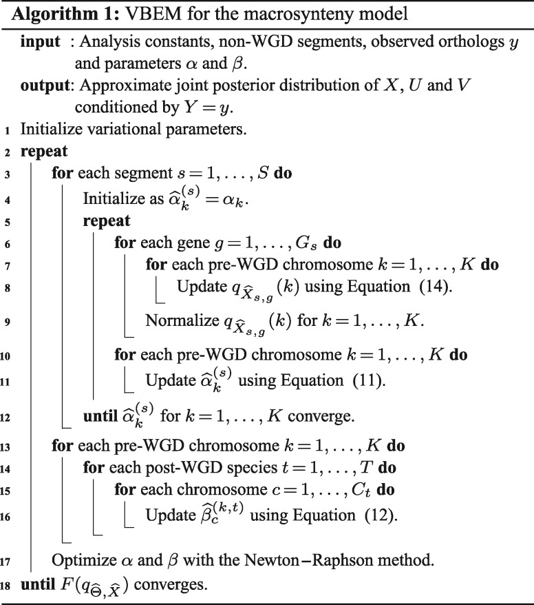
Finally, using the update formulas above, we obtain the VBEM algorithm for the macrosynteny model as Algorithm 1. The Newton–Raphson method for optimizing hyper-parameters, parameter initialization and convergence criteria are described in Supplementary Material Sections S7.4, S7.5 and S7.6, respectively.
4 Results
4.1 Simulation of the macrosynteny model
In order to evaluate the estimation accuracy, we generated synthetic ortholog data from the generative model described in Sections 2.2 to 2.4 with and . First, we set () and ( and ), where either a or b was fixed to 0.1 and the other parameter was varied from 0.01 to 1. Second, we generated segments and chose the number of genes for each segment from the exponential distribution with parameter , which approximates the actual distribution of human segment length. Third, we chose values of Us () and ( and ) randomly from their prior distributions: namely, the symmetric Dirichlet distributions with parameters a and b, respectively. Forth, we generated orthologs from the categorical distributions Us and as shown in Figure 1H, where two post-WGD orthologs were generated for each non-WGD gene with probability 0.1. After applying the macrosynteny model algorithm, estimates for all non-TGD segments were compared with the true values , where k is chosen for each s as . Then, estimation accuracy was evaluated in terms of three quantities: (A) Pearson’s correlation coefficient between simulated and estimated values, (B) mean absolute estimation error defined by with and (C) proportion of non-WGD genes that are in segments with correct inference (i.e. segments s satisfying ). This simulation procedure was repeated 20 times for each set of parameter values.
Overall, the simulation result (Fig. 2) shows that the algorithm gave accurate estimates. In addition, we confirmed factors that affect the inference accuracy. First, shorter non-WGD segments tend to have larger estimation errors. Specifically, segment length (i.e. number of genes in the segment) negatively correlated with estimation error with (Spearman’s rank correlation coefficient was –0.51 when and ). Second, accuracy is dependent on genome rearrangements in both non- and post-WGD lineages. Indeed, by increasing a and b parameter values, which represent degrees of genome shuffling in non- and post-WGD genomes respectively, we observed a decrease in the correlation coefficient and an increase in the mean absolute estimation error (Fig. 2A and B).
Fig. 2.

High estimation accuracy of the macrosynteny model algorithm. (A) Simulations showed strong correlation between true and estimated values (i.e. and with ). A parameter value (either a or b) was varied from 0.01 to 1 (x-axis) and Pearson’s correlation coefficient is shown on the y-axis with 25% and 75% quantiles indicated by boxes. Correlation was strong in general, although the correlation coefficient was relatively low for . (B) The estimation error was larger for more rearranged genomes. The mean absolute estimation error (y-axis) was small especially for small a or b values (x-axis), which correspond to low rates of rearrangement in non- and post-WGD genomes, respectively. (C) The association with pre-WGD chromosomes was accurately inferred for most non-WGD segments. The y-axis shows the proportion of non-WGD genes that are in segments with correct inference
Importantly, the influence of these factors seems to be minimal in the actual teleost genome analysis for three reasons: short segments were not used in the initialization step (see Supplementary Material Section S7.5); most synteny breakpoints were detected accurately by using a Bayesian segmentation algorithm (see Section 4.2.1); and post-TGD genomes are known to have had low rates of inter-chromosomal rearrangement (Jaillon et al., 2004; Kasahara et al., 2007). In fact, in our teleost genome analysis, the average αk and values were estimated to be and (averaged with respect to all values of k, t and c) using the Newton–Raphson method described in Supplementary Material Section S7.4. Figure 2 shows high estimation accuracy for these parameter values.
4.2 Analysis of the teleost WGD
4.2.1 Reconstruction of the pre-TGD genome structure
We obtained vertebrate orthologs and gene trees from Ensembl (release 75) and removed small-scale duplications to avoid ambiguity in subsequent synteny analyses. In other words, duplications were retained only if they were annotated as Clupeocephala (indicating that the duplication events occurred to the last common ancestor of teleost species in Ensembl), and the other duplications were removed. Then we compared four teleosts (medaka, stickleback, Tetraodon and zebrafish), spotted gar, four non-mammalian amniotes (chicken, zebra finch, turkey and anole lizard), and four mammals (opossum, dog, mouse and human) to define conserved synteny blocks in the human, mouse, dog, opossum, anole lizard, chicken and spotted gar genomes. Specifically, we employed a Bayesian segmentation model (Liu and Lawrence, 1999) with a dynamic programming algorithm for computing the maximum a posteriori segmentation (Auger and Lawrence, 1989). In short, the segmentation algorithm identifies synteny breakpoints and divides chromosomes, represented as sequences of genes, into chromosomal segments each of which is characterized by a homogeneous ortholog distribution in the genomes under comparison. The segmentation algorithm was applied twice to the human genome: first, for identifying boundaries of teleost synteny blocks (i.e. blocks of doubly conserved synteny, Jaillon et al., 2004) by using the four teleost genomes; second, for identifying boundaries of amniote synteny blocks by using the four non-mammalian amniote genomes. Then, by merging the two sets of boundaries, the human genome was partitioned into 152 segments. In the same way, the mouse, dog, opossum, anole lizard, chicken and spotted gar genomes were partitioned into 252, 209, 159, 77, 71 and 78 segments, respectively. This construction allows us to assume that the resulting segments have been conserved and mostly free from large-scale inter-chromosomal rearrangements among the non-TGD species and pre-TGD ancestor.
These segments and Ensembl orthologs were used as the input data for the macrosynteny model algorithm. We present the result in Figure 3, which was obtained by the macrosynteny model algorithm with parameters (), ( and ), , , for all t, and , where L is explained in Supplementary Material Section S7.5. Visualization scheme is described in the figure legend.
Fig. 3.

Reconstruction of the pre-TGD genome structure comprising of 13 chromosomes. We assigned distinct colors to the pre-TGD chromosomes and painted the post- and non-TGD chromosomes accordingly. Specifically, the non-TGD segments were painted with the color of the pre-TGD chromosome that had the maximum reconstruction confidence score (i.e., ). To visualize local reconstruction confidence, lines were drawn by weighted window averaging of for genes in the surrounding W Mb regions ( and 0.48 for human, mouse, dog, chicken and spotted gar, respectively, reflecting their genome size difference). Lines are visible only when there exists at least one gene in the window, and local confidence scores are shown in the range from 0.3 to 1. With regard to the post-TGD genomes, lines were drawn by weighted window averaging of gene-wise reconstruction confidence values, where gene-wise reconstruction confidence of a post-TGD gene was calculated by averaging of all segments that contain non-TGD orthologs since reconstruction probability was not assigned to post-WGD genes within the model. The window sizes were 0.44, 0.23, 0.18 and 0.7 Mb for medaka, stickleback, Tetraodon and zebrafish, respectively. Then, post-TGD chromosomes were painted with the color associated with the pre-TGD chromosome that had the maximum window average value. Chromosome length is proportionate within each species, but do not scale between species. In the main text, chromosome numbers were prefixed by three letter codes (i.e. Ola, Tni and Hsa for medaka, Tetraodon and human, respectively)
4.2.2 Number of pre-TGD chromosomes
The number of pre-TGD chromosomes (denoted by K in the macrosynteny model) has been estimated as (Jaillon et al., 2004) or (Kasahara et al., 2007), but the exact number remains unknown. We reconstructed the pre-TGD chromosomes for and compared with the case shown in Figure 3 to see how reconstructions are affected by the choice of K.
In order to decide the true number of chromosomes, it is important to discern the difference between ortholog distributions produced by chromosome fusion and fission. For example, in Figure 1 the post-TGD species has a fusion chromosome (chr4, fusion of yellow and green chromosomes). In this case, we can see that yellow non-TGD segments share orthologs with chr3 and chr4 but not with chr5, while green non-TGD segments share orthologs with chr4 and chr5 but not with chr3 (except for a small number of translocated genes). On the other hand, chr7 and chr8 (blue chromosomes) were created by fission, and consequently some blue non-TGD segments are syntenic to the three blue post-TGD chromosomes (chr6, chr7 and chr8). Therefore, chromosome fusion and fission can be distinguished by the existence of many non-TGD segments that are syntenic to three post-TGD chromosomes. This distinction can be obscured by inter-chromosomal rearrangements, and thus we focused on ortholog distribution in medaka with a low rate of inter-chromosomal rearrangement (Kasahara et al., 2007).
When we increased K from to , a pre-TGD chromosome was divided into two chromosomes (namely, chr10 and chr11 in Figure 3 with 57 and 38 non-TGD segments, respectively). Investigation of medaka ortholog distribution showed that these segments are syntenic to either Ola3-Ola6 pair or Ola23-Ola6 pair of medaka chromosomes (Fig. 4A), which is expected under the fusion scenario (i.e. the three medaka chromosomes derive from two pre-TGD chromosomes and Ola6 is a fusion chromosome). This observation suggests that the true number of chromosomes in the pre-TGD genome is more than 11 and setting caused the false merger of two pre-TGD chromosomes (chr10 and chr11 in Fig. 3) into one in the reconstruction. Similarly, when we increased the number from to , a pre-TGD chromosome (namely, chr13 in Fig. 3 with 159 non-TGD segments) was divided into two chromosomes. The medaka ortholog distribution (Fig. 4B) showed that many segments are syntenic to both Ola3 and Ola23 (in addition to Ola17), which is expected under the fission scenario (i.e. the three medaka chromosomes derive from a single pre-TGD chromosome, where Ola4 and Ola20 were separated by fission). Thus, it is likely that the reconstructions with have falsely inferred two pre-TGD chromosomes where there really should be one. Taken together, Figure 4 supports the reconstructions with and 13.
Fig. 4.
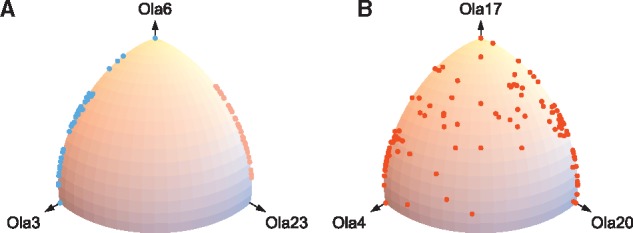
Two contrasting patterns were observed for ortholog distributions over three medaka chromosomes produced by fusion (A) or fission (B). For each non-TGD segment, we counted the numbers of orthologs in the three medaka chromosomes shown in the x, y and z axes (Ola stands for Oryzias latipes chromosome). The three-dimensional count vector was projected onto the sphere to show the proportion of orthologs among the three chromosomes. (A) Ortholog distribution consistent with the fusion scenario. Non-TGD segments assigned to pre-TGD chromosomes chr10 and chr11 were plotted in light blue and pink, respectively. Ola6 is likely to have been produced by fusion of two chromosomes, one duplicated from chr10 and the other from chr11. Consequently, any non-TGD segments syntenic to Ola6 are also syntenic to either Ola3 or Ola23, but no segment is syntenic to both of Ola3 and Ola23. (B) Ortholog distribution consistent with the fission scenario. Non-TGD segments assigned to pre-TGD chromosome chr13 were plotted. Ola4 and Ola20 are likely to have been created by fission of a chromosome that was a duplicate of Ola17. Since the three medaka chromosomes are derived from a single pre-TGD chromosome, many non-TGD segments are syntenic to both Ola4 and Ola20 in addition to Ola17
The difference between and reconstructions involves several post-TGD chromosomes (i.e. Ola1, Ola18, Ola10 and Ola14), suggesting a complicated rearrangement history after TGD. Further comparison with previously proposed rearrangement scenarios (Jaillon et al., 2004; Kasahara et al., 2007) showed that the model proposed by Jaillon et al. is not consistent with our reconstruction (e.g. assignment of Tetraodon chromosomes Tni6 and Tni17 to pre-TGD chromosomes differs), while the model proposed by Kasahara et al. largely agrees with our reconstruction. In addition, Ola1 and Ola14 have orthologs in non-overlapping regions in the non-TGD genomes (e.g. see Supplementary Fig. S8), supporting the inference that the two chromosomes derive from two distinct pre-TGD chromosomes as in the reconstruction. Considering these observations, we presented the reconstruction with in the main text and an alternative reconstruction with in the supplementary document. These reconstructions may be validated by comparison with genomes of basally diverging post-TGD species such as African butterfly fish and arowana. For example, Ola4 and Ola20 are syntenic to the same chromosome (chr12) in golden arowana (Bian et al., 2016), suggesting that Ola4 and Ola20 were indeed created by chromosome fission (as discussed in Fig. 4B) after divergence from the arowana lineage.
4.2.3 Evolution of genome structure in teleost
Figure 3 shows that the inferred structure of the pre-TGD genome is largely consistent with the previous reconstructions presented in (Jaillon et al., 2004; Kasahara et al., 2007), confirming their findings on teleost genome evolution: (1) after the TGD, the rate of inter-chromosomal rearrangement has been relatively low in the teleost genomes compared with the mammalian genomes; (2) in medaka, stickleback and Tetraodon, only a small number of chromosome fusion or fission events have occurred since the TGD, and the other chromosomes have retained one-to-one correspondence; and (3) by contrast, many inter-chromosomal rearrangements have occurred in the zebrafish lineage, presumably because of increased activity of transposable elements as argued in (Jaillon et al., 2004).
The major difference of our reconstruction from previous ones is that we have increased the coverage of the genomes and assigned confidence scores along chromosomal regions for representing uncertainty in reconstruction, whereas previous studies had excluded a large part of the human genome from their reconstructions to avoid regions with ambiguous synteny (for example, Jaillon et al. excluded 20 blocks in the human genome. See Fig. 6 in Jaillon et al., 2004). In many cases, previously excluded regions were divided into several smaller blocks with varying degree of confidence in our reconstruction (see Fig. 6 in Jaillon et al., 2004, blocks W1, Z1, Z3, etc).
As a result, our reconstruction shows previously unidentified small-scale rearrangements occurring after the TGD. For instance, Ola18 and Ola22 were considered in (Kasahara et al., 2007) to have been free of large-scale inter-chromosomal rearrangements since the TGD, except for a small translocation from Ola18 to Ola10; by contrast, in Figure 3, Ola18 (purple) and Ola22 (light green) are the most rearranged chromosomes in medaka, having experienced several small-scale rearrangements as indicated by short segments painted in several different colors. Thus, even though the medaka genome in general has been characterized by a low rate of inter-chromosomal rearrangement after the TGD (Kasahara et al., 2007), our reconstruction indicates that some chromosomes experienced substantially higher rates of rearrangement, which suggests relatively weak structural constraints or local expansion of repetitive sequences.
4.2.4 Evolution of genome structure in vertebrate
Comparison of the pre- and non-TGD genomes in Figure 3 revealed macrosynteny evolution before the TGD: (1) large chromosomes in chicken and spotted gar tend to consist of multiple segments painted in different combinations of colors, suggesting that these chromosomes were formed by inter-chromosomal rearrangements (possibly by fusion of smaller chromosomes) in the individual lineages; (2) by contrast, many of chicken microchromosomes (i.e. smaller chromosomes such as Gga9 to Gga32) have retained one-to-one correspondence to the spotted gar chromosomes (Braasch et al., 2016; see also Supplementary Fig. S8), but none of them were retained as single chromosomes in the pre-TGD genome, indicating a large number of chromosomes in the common ancestor and fusion events in the pre-TGD lineage; and (3) all pre-TGD chromosomes except for chr11 (pink) are divided into smaller parts and distributed to multiple chromosomes in chicken and spotted gar. These observations corroborate a previously proposed model that the bony-vertebrate ancestor had a large number of chromosomes and intensive chromosome fusion events shaped the pre-TGD genome structure (Nakatani et al., 2007). Intriguingly, one of ancestral chromosomes created by the vertebrate WGDs (Nakatani et al., 2007) had been retained in the pre-TGD genome as a single chromosome (namely, chr11 painted in pink), surviving the period when the other ancestral chromosomes underwent fusion to form pre-TGD chromosomes. This linkage conservation might suggest that pre-TGD chr11 had been under strong structural constraint.
Taken together, our reconstruction with higher resolution helps refine previous models of genome evolution in teleost and vertebrate. In particular, it has been highlighted that some lineages had remarkably slow rates of large-scale inter-chromosomal rearrangement for a long evolutionary time, while other lineages had intensive chromosome fusions in a short evolutionary time (Jaillon et al., 2004; Kasahara et al., 2007; Nakatani et al., 2007). Our reconstruction refines this view by showing that (1) some chromosomes might have accumulated small-scale inter-chromosomal rearrangements even in a slowly evolving genome and (2) by contrast, some might have experienced exceptionally strong structural constraints and retained ancestral linkage even in a rapidly changing genome.
5 Discussion
We considered that reconstructions computed independently by previous algorithms might be useful in validating and also improving our reconstruction. In particular, we presumed that previous gene-order reconstruction algorithms can infer reliable fragments of pre-TGD chromosomes; then (1) those fragments can be used for validating our macrosynteny-based reconstruction, or alternatively (2) those fragments can be treated as input to the macrosynteny model algorithm for obtaining an improved reconstruction of the pre-TGD genome structure.
For this purpose, we have chosen GapAdj (Gagnon et al., 2012), a sophisticated algorithm designed for reconstructing ancestral genomes in yeasts and plants. The major advantage of GapAdj (compared with other gene-order reconstruction algorithms) is that it takes account of gene duplications by WGDs and subsequent gene deletions, which are essential for the analysis of the TGD. The GapAdj algorithm reconstructs contiguous ancestral regions (CARs) based on gene adjacencies in modern genomes, where a gene is represented as two extremities (i.e., start and end) and a pair of genes is regarded as adjacent if there are less than or equal to a given number (denoted by δ) of gene extremities between the pair. With a small number of δ, GapAdj produces numerous short CARs, representing fragments of ancestral chromosomes; on the other hand, with a large number of δ, GapAdj reconstructs entire ancestral chromosomes at the cost of reconstruction accuracy (Gagnon et al., 2012).
First, we evaluated whether GapAdj is capable of reconstructing entire pre-TGD chromosomes and validating our reconstruction. To this end, we obtained gene order information from the human, mouse, dog, chicken, spotted gar, medaka, stickleback, Tetraodon and zebrafish genomes, and applied GapAdj with . Figure 5A shows that GapAdj generated considerably larger numbers of CARs (116 CARs with the least stringent ) than the expected pre-TGD chromosome number (), indicating that gene-order conservation was not sufficiently strong for recovering the gene order along entire pre-TGD chromosomes.
Fig. 5.

Gene-order reconstruction of the pre-TGD genome by GapAdj. (A) The number of pre-TGD CARs remained larger than the expected chromosome number even with less stringent large δ values. The x-axis shows the value of δ, and the y-axis shows the number of CARs reconstructed by GapAdj. The plot shows three data series: first, we analyzed gene order in the human, medaka and Tetraodon genomes (); second, we added mouse, dog, chicken, spotted gar, zebrafish and stickleback (); third, we analyzed only the spotted gar genome and the four teleost genomes (+). In all cases, the number of CARs was too large, indicating that reconstruction of entire pre-TGD chromosomes was not feasible presumably due to a weak gene-order conservation. (B) Ortholog distribution over medaka chromosomes suggested that large CARs were likely to be unreliable. CARs inferred by GapAdj with and 100 (data series in panel A) were plotted, where the x-axis shows the number of genes in the CARs and the y-axis shows the proportion of their orthologs located on the two most syntenic medaka chromosomes. Large y-axis values were expected if CARs were inferred accurately, because majority of their medaka orthologs should be found in two duplicated chromosomes. The top panel shows that GapAdj reconstructed only short fragments with , indicating that the value was too stringent for teleost genome analysis. On the other hand, larger CARs were inferred by using less stringent and 100 (middle panels). However, compared with large y-axis values for the non-TGD segments (bottom), relatively low y-axis values for large CARs indicate that presently available gene-order information was not sufficient for accurate reconstruction of large CARs
Next, to see if our reconstruction improves by integrating GapAdj, we applied the macrosynteny model algorithm to the 116 CARs with parameters chosen to be the same as in our teleost genome analysis (Section 4.2). Assuming that the CARs were inferred accurately, we expected that most genes in a single CAR should belong to a single pre-TGD chromosome, resulting in small αk and large estimates. However, we found the opposite tendency: first, the average of the estimated αk values was 0.154 for the CARs, which was larger than the average of 0.066 in our teleost genome analysis; and second, values of were considerably smaller for the CARs (0.51 on average) than the non-TGD segments in our teleost genome analysis (0.78 on average). Although no statistical test was performed because of dependence of the estimates, the result indicated that the CARs were more ‘rearranged’ than the non-TGD segments, suggesting that the CARs might not have been reconstructed with sufficient accuracy.
In accord with this argument, we observed that the CARs tend to have orthologs in more than two medaka chromosomes. Ideally, if a CAR was reconstructed accurately, all genes in the CAR must have been on the same pre-TGD chromosome and consequently most of their medaka orthologs should be found on two duplicated chromosomes (although some genes might have moved away by rearrangement). Therefore, we quantified accuracy of a CAR in terms of the proportion of its medaka orthologs located on the two most syntenic chromosomes (i.e. the two chromosomes that have the largest and second largest numbers of orthologs in the CAR) as shown on the y-axes in Figure 5B. The proportion was significantly lower for the 116 CARs inferred by GapAdj with than for the 152 non-TGD segments in human (59% and 86% on average for the CARs and human segments, respectively; , Mann–Whitney U test). This indicates that gene-order conservation was not strong enough for reliable reconstruction of large CARs.
In fact, our observation was consistent with the previous argument that inference accuracy of GapAdj was reduced by high rates of rearrangement and gene loss in simulations (Gagnon et al., 2012). Taken together, the present analysis indicates that gene-order conservation is not sufficiently strong among the non- and post-TGD genomes, making a reliable inference of pre-TGD gene order infeasible even with advanced algorithms like GapAdj (see Supplementary Material Section S7.7 for confirmation of this observation using other gene-order reconstruction methods).
Although we could not improve our reconstruction at present by integrating a gene-order reconstruction method, such a hybrid approach is potentially useful in future teleost and vertebrate genome analyses. Future work should also include (1) improving the method for detecting synteny blocks by using gene-order reconstruction methods and comparing with many low-coverage genome sequences, (2) developing more realistic probability models of rearrangement and macrosynteny evolution and (3) applying other document models and algorithms to the problem of ancestral genome reconstruction.
6 Conclusion
We have developed a probabilistic macrosynteny model and inferred the structure of the pre-TGD genome. Unlike previous studies (e.g. Jaillon et al., 2004; Kasahara et al., 2007), which had a drawback that their reconstructions lack a quantified level of confidence (Muffato and Roest Crollius, 2008), we have calculated reconstruction confidence scores along chromosomes of present-day genomes, representing reconstruction uncertainty due to intensive local rearrangements, incomplete genome sequencing, errors in identifying synteny breakpoints, errors in gene trees, etc.
The major difference between our method and previous gene-order-based algorithms is that the macrosynteny model is abstract and does not directly model actual evolutionary processes: specifically, it focuses on ortholog distribution rather than conservation of gene order or gene adjacency. This has been an essential idea underlying previous studies (Jaillon et al., 2004; Kasahara et al., 2007; Muffato, 2010; Nakatani et al., 2007; Putnam et al., 2007; Putnam et al., 2008). We have formulated the idea into a rigorous probabilistic framework (Section 2), and as a result, our method works effectively (Section 4.2) even in a situation where gene-order reconstruction algorithms do not work reliably (Section 5) due to ancient occurrence of WGDs and high rates of rearrangement and gene loss.
Finally, the similarity between the macrosynteny and topic models (Blei et al., 2003; Blei, 2012; Murphy, 2012) suggests an interesting interpretation of conserved synteny: that is, a block of conserved synteny can be regarded as a piece of writing about local structure of ancestral genomes. Consequently, by compiling and summarizing those ‘documents’ using an algorithm originally developed for text analyses, we were able to recover the ancestral genome structure as if we inferred the ‘topic structure’ underlying the macrosynteny ‘documents.’ Viewed in this way, the present study provides a perfect example of the prevalent metaphor that genomes are documents of evolutionary history (Boussau and Daubin, 2010; Crow, 1994; Kihara, 1946; Zuckerkandl and Pauling, 1965).
Supplementary Material
Acknowledgement
We thank all members of the McLysaght research group for valuable discussions.
Funding
This work is supported by funding from the European Research Council under the European Union’s Seventh Framework Programme (FP7/2007–2013)/European Research Council grant agreement 309834.
Conflict of Interest: none declared.
References
- Auger I., Lawrence C. (1989) Algorithms for the optimal identification of segment neighborhoods. Bull. Math. Biol., 51, 39–54. [DOI] [PubMed] [Google Scholar]
- Bian C. et al. (2016) The Asian arowana (Scleropages formosus) genome provides new insights into the evolution of an early lineage of teleosts. Sci. Rep., 6, 24501. [DOI] [PMC free article] [PubMed] [Google Scholar]
- Blei D.M. et al. (2003) Latent Dirichlet allocation. J. Mach. Learn. Res., 3, 993–1022. [Google Scholar]
- Blei D.M. (2012) Probabilistic topic models. Commun. ACM, 55, 77–84. [Google Scholar]
- Boussau B., Daubin V. (2010) Genomes as documents of evolutionary history. Trends Ecol. Evol., 25, 224–232. [DOI] [PubMed] [Google Scholar]
- Braasch I. et al. (2016) The spotted gar genome illuminates vertebrate evolution and facilitates human-teleost comparisons. Nat. Genet., 48, 427–437. [DOI] [PMC free article] [PubMed] [Google Scholar]
- Crow J.F. (1994) Hitoshi Kihara, Japan’s pioneer geneticist. Genetics, 137, 891–894. [DOI] [PMC free article] [PubMed] [Google Scholar]
- El-Mabrouk N. et al. (1998) Genome halving. In Combinatorial Pattern Matching, Lect. Notes Comput. Sci., 1448, 235–250. [Google Scholar]
- El-Mabrouk N., Sankoff D. (2003) The reconstruction of doubled genomes. SIAM J. Comput., 32, 754–792. [Google Scholar]
- El-Mabrouk N., Sankoff D. (2012) Analysis of gene order evolution beyond single-copy genes In: Evolutionary Genomics, Methods Mol. Biol. Humana Press, pp. 397–429. [DOI] [PubMed] [Google Scholar]
- Gagnon Y. et al. (2012) A flexible ancestral genome reconstruction method based on gapped adjacencies. BMC Bioinform., 13, S4.. [DOI] [PMC free article] [PubMed] [Google Scholar]
- Gavranović H. et al. (2011) Mapping ancestral genomes with massive gene loss: a matrix sandwich problem. Bioinformatics, 27, i257–i265. [DOI] [PMC free article] [PubMed] [Google Scholar]
- Gordon J.L. et al. (2009) Additions, losses, and rearrangements on the evolutionary route from a reconstructed ancestor to the modern Saccharomyces cerevisiae Genome. PLoS Genet., 5, e1000485. [DOI] [PMC free article] [PubMed] [Google Scholar]
- Holland P.W.H. (1998) Major transitions in animal evolution: a developmental genetic perspective. Am. Zool., 38, 829–842. [Google Scholar]
- Jahn K. et al. (2012) A consolidation algorithm for genomes fractionated after higher order polyploidization. BMC Bioinform., 13, S8.. [DOI] [PMC free article] [PubMed] [Google Scholar]
- Jaillon O. et al. (2004) Genome duplication in the teleost fish Tetraodon nigroviridis reveals the early vertebrate proto-karyotype. Nature, 431, 946–957. [DOI] [PubMed] [Google Scholar]
- Kasahara M. et al. (2007) The medaka draft genome and insights into vertebrate genome evolution. Nature, 447, 714–719. [DOI] [PubMed] [Google Scholar]
- Kihara H. (1946) Story on Wheats. Sogen-sha; Tokyo. [Google Scholar]
- Liu J.S., Lawrence C.E. (1999) Bayesian inference on biopolymer models. Bioinformatics, 15, 38–52. [DOI] [PubMed] [Google Scholar]
- Makino T., McLysaght A. (2010) Ohnologs in the human genome are dosage balanced and frequently associated with disease. Proc. Natl. Acad. Sci. USA, 107, 9270–9274. [DOI] [PMC free article] [PubMed] [Google Scholar]
- Makino T. et al. (2013) Genome-wide deserts for copy number variation in vertebrates. Nat. Commun., 4, 2283. [DOI] [PubMed] [Google Scholar]
- McLysaght A. et al. (2014) Ohnologs are overrepresented in pathogenic copy number mutations. Proc. Natl. Acad. Sci. USA, 111, 361–366. [DOI] [PMC free article] [PubMed] [Google Scholar]
- Muffato M. (2010) Reconstruction de génomes ancestraux chez les vertébrés. PhD Thesis, Université d’Evry-Val d’Essonne, Evry, France.
- Muffato M., Roest Crollius H. (2008) Paleogenomics in vertebrates, or the recovery of lost genomes from the mist of time. BioEssays, 30, 122–134. [DOI] [PubMed] [Google Scholar]
- Murphy K.P. (2012) Machine Learning: A Probabilistic Perspective. MIT Press, Cambridge. [Google Scholar]
- Nakatani Y. et al. (2007) Reconstruction of the vertebrate ancestral genome reveals dynamic genome reorganization in early vertebrates. Genome Res., 17, 1254–1265. [DOI] [PMC free article] [PubMed] [Google Scholar]
- Ohno S. (1970) Evolution by Gene Duplication. Springer-Verlag, New York. [Google Scholar]
- Ouangraoua A. et al. (2009) Prediction of contiguous regions in the amniote ancestral genome. Lect. Notes Comput. Sci., 5542, 173–185. [Google Scholar]
- Ouangraoua A. et al. (2011) Reconstructing the architecture of the ancestral amniote genome. Bioinformatics, 27, 2664–2671. [DOI] [PubMed] [Google Scholar]
- Putnam N.H. et al. (2007) Sea anemone genome reveals ancestral eumetazoan gene repertoire and genomic organization. Science, 317, 86–94. [DOI] [PubMed] [Google Scholar]
- Putnam N.H. et al. (2008) The amphioxus genome and the evolution of the chordate karyotype. Nature, 453, 1064–1071. [DOI] [PubMed] [Google Scholar]
- Rice A.M., McLysaght A. (2017) Dosage sensitivity is a major determinant of human copy number variant pathogenicity. Nat. Commun., 8, 14366.. [DOI] [PMC free article] [PubMed] [Google Scholar]
- Sankoff D. et al. (2007) Polyploids, genome halving and phylogeny. Bioinformatics, 23, i433–i439. [DOI] [PubMed] [Google Scholar]
- Scannell D.R. et al. (2006) Multiple rounds of speciation associated with reciprocal gene loss in polyploid yeasts. Nature, 440, 341–345. [DOI] [PubMed] [Google Scholar]
- Van de Peer Y. et al. (2009) The evolutionary significance of ancient genome duplications. Nat. Rev. Genet., 10, 725–732. [DOI] [PubMed] [Google Scholar]
- Wolfe K. (2000) Robustness? it’s not where you think it is. Nat. Genet., 25, 3–4. [DOI] [PubMed] [Google Scholar]
- Zheng C. et al. (2008) Guided genome halving: hardness, heuristics and the history of the Hemiascomycetes. Bioinformatics, 24, i96–i104. [DOI] [PMC free article] [PubMed] [Google Scholar]
- Zheng C., Sankoff D. (2013) Practical aliquoting of flowering plant genomes. BMC Bioinform., 14, 1–8. [DOI] [PMC free article] [PubMed] [Google Scholar]
- Zuckerkandl E., Pauling L. (1965) Molecules as documents of evolutionary history. J. Theor. Biol., 8, 357–366. [DOI] [PubMed] [Google Scholar]
Associated Data
This section collects any data citations, data availability statements, or supplementary materials included in this article.