Abstract
Modern digital pathology departments have grown to produce whole-slide image data at petabyte scale, an unprecedented treasure chest for medical machine learning tasks. Unfortunately, most digital slides are not annotated at the image level, hindering large-scale application of supervised learning. Manual labeling is prohibitive, requiring pathologists with decades of training and outstanding clinical service responsibilities. This problem is further aggravated by the United States Food and Drug Administration’s ruling that primary diagnosis must come from a glass slide rather than a digital image. We present the first end-to-end framework to overcome this problem, gathering annotations in a nonintrusive manner during a pathologist’s routine clinical work: (i) microscope-specific 3D-printed commodity camera mounts are used to video record the glass-slide-based clinical diagnosis process; (ii) after routine scanning of the whole slide, the video frames are registered to the digital slide; (iii) motion and observation time are estimated to generate a spatial and temporal saliency map of the whole slide. Demonstrating the utility of these annotations, we train a convolutional neural network that detects diagnosis-relevant salient regions, then report accuracy of 85.15% in bladder and 91.40% in prostate, with 75.00% accuracy when training on prostate but predicting in bladder, despite different pathologists examining the different tissues. When training on one patient but testing on another, AUROC in bladder is 0.79±0.11 and in prostate is 0.96±0.04. Our tool is available at https://bitbucket.org/aschaumberg/deepscope
1 Scientific Background
Computational pathology [12] relies on training data annotated by human experts on digital images. However, the bulk of a pathologist’s daily clinical work remains manual on analog light microscopes. A noninterfering system which translates this abundance of expert knowledge at the microscope into labeled digital image data is desired.
Tracking a pathologist’s viewing path along the analyzed tissue slide to detect local image saliency has been previously proposed. These approaches include whole slide images displayed on one or more monitors with an eye-tracker [5], mouse-tracker [21] or viewport-tracker [19, 23] – but may suffer confounds including peripheral vision [18], head turning [1], distracting extraneous detail [2], monitor resolution [22], multimonitor curvature [25], and monitor bezel field of view fragmentation [27]. Because computer customizations may potentially effect viewing times, for studies of pathologists recorded at a computer, we suggest noting the sensitivity and choice of pointing device, e.g. trackball, touch pad, touch screen, pointing stick, mouse, and if a scroll wheel or keyboard was available to zoom in or out. Only our approach does not change the pathologist’s medical practice from the microscope. The microscope is a class I device appropriate for primary diagnosis according to the United States Food and Drug Administration, while whole slide imaging devices are class III [20].
In light of the confounds of alternatives, its centuries of use in pathology, and its favorable regulatory position for primary diagnosis, we believe the microscope is the gold standard for measuring image region saliency. Indeed, there is prior work annotating regions of interest at the microscope for cytology technicians to automatically position the slide for a pathologist [4].
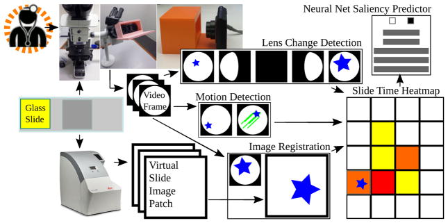
We therefore propose a new, noninterfering workflow for automated video-based detection of region saliency using pathologist viewing time at the microscope (Fig 1). Viewing time is known in the psychology literature to measure attention [8, 15], and we define saliency as pathologist attention when making a diagnosis. Using a commodity digital camera, rather than a custom embedded eye-tracking device [7, 16], we video record the pathologist’s entire field of view at a tandem microscope to obtain slide region viewing times and register these regions to whole slide image scan regions. Second, we train a convolutional neural network [CNN] on these observation times to predict whether or not a whole slide image region is viewed by a pathologist at the microscope for more than 0.1 seconds [s]. As more videos become available, our CNN predicting image saliency may be further trained and improved, through online learning.
Fig. 1.
Proposed microscope-based saliency predictor pipeline workflow. The pathology session is recorded, the slide is scanned, the video frames are registered to scan patches. Lens change detection guides registration and viewing time is recorded for periods without motion. A convolutional neural net learns to classify patches as salient (long looks) or not.
2 Materials and Methods
Pathologists
Pathologists were assistant attending rank with several years experience each. Trainees have different, less efficient, slide viewing strategies [5, 18]. Region viewing times and path were automatically recorded during a pathologist’s routine slide analysis, without interference.
Patient slides
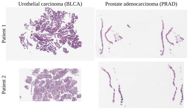
Two bladder cancer patients were studied by author SJS. Two prostate cancer patients were studied by author HAA. One slide per patient was used, for four slides total (Fig 2).
Fig. 2.
Bladder cancer left, prostate cancer right. Training, validation, testing done on top slides, with additional same-tissue testing on bottom slides. For cross-tissue testing, top slide tested against other top slide. Viewing time heatmap for top left bladder shown in Fig 7. Note how the top bladder has more edges than the more solid bottom bladder, while the prostates have similar tissue texture. We believe this impacts interpatient accuracy, shown in Fig 9.
Scan preprocessing
Microscope slides, inspected by a pathologist, were scanned at 0.5±0.003 microns per pixel [px], using an Aperio AT2 scanner. The resulting SVS data file consists of multiple levels, where level 0 is not downsampled, level 1 is downsampled by a factor of 4, level 2 by a factor of 16, and level 3 by a factor of 32. From each level, 800 × 800 px patches were extracted via the OpenSlide software library [13]. In bladder, adjacent patches in a level overlap at least 50%, to avoid windowing artifacts in registration. In prostate, adjacent patches overlap at least 75%, to best center the pathologist’s field of view on the little tissue in a needle biopsy. Patches evenly cover the entire level without gaps. Scans were either taken before a technician applied marker to the slides, to indicate regions of interest to the pathologist, or after markings were scrubbed from the slide. However, these marks were evident in the pathologist videos discussed in the next section.
Video acquisition
A Panasonic Lumix DMC-FH10 camera with a 16.1 megapixel charge-coupled device [CCD], capable of 720p motion JPEG video at 30 frames per second fps], was mounted on a second head of an Olympus BX53F multihead teaching microscope to record the pathologist’s slide inspection. Microscope objective lens magnifications were 4x, 10x, 20x, 40x, and 100x. Eyepiece lens magnifications was 10x. The pathologist was told to ignore the device and person recording video at the microscope during inspection. The mount (Fig 1) for this camera was designed in OpenSCAD and 3D-printed on a MakerBot 2 using polylactic acid [PLA] filament.
Camera choice
Many expensive microscope-mounted cameras exist, such as the Lumenera INFINITY-HD and Olympus DP27, which have very good picture quality and frame rate. The Lumenera INFINITY-HD is a CMOS camera, not CCD, so slide movement will skew the image rather than blur it, and we did not want to confound image registration or motion detection with rolling shutter skew. Both cameras trim the field of view to a center-most rectangle for viewing on a computer monitor, which is a loss of information, and we instead assign viewing time to the entire pathologist-viewed 800×800 px PNG patch from the SVS file representing the whole slide scan image. Both cameras do not have USB or Ethernet ports carrying a video feed accessible as a webcam, for registration to the whole slide scan. The Olympus DP27 may be accessible as a Windows TWAIN device, but we could not make this work in Linux. Finally, the HDMI port on both carries high-quality but encrypted video information that we cannot record, and we did not wish to buy a Hauppauge HDMI recording device, because we had a cheaper commodity camera on hand already. We also considered automated screenshots of the video feed in Aperio ImageScope as displayed on a computer monitor, but we observed a lower frame rate and detecting lens change is complicated because the entire field of view is not available. Recording low-quality video on a commodity camera to a SecureDigital [SD] memory card is inexpensive, captures the entire field of view, and is generally applicable in any hospital. For this pilot study, we used only one camera for video recording, rather than two different microscope cameras, potentially eliminating a confound for how many pixels are moving during rapid short movements of the slide. For 3D printing requisite camera mounts, open source tools are available.
Video preprocessing and registration
A Debian Linux computer converted individual slide inspection video frames to PNG files using the ffmpeg program. OpenCV software detected slide movement via a dense optical flow procedure [9, 10], comparing the current and preceding video frames, shown in Fig 3. Through this dense optical flow procedure. we calculated a movement vector for each pixel of each camera video frame, where a movement vector magnitude of one means the pixel has been displaced by one pixel in the video frame of interest, with respect to the previous video frame. Though the details of this procedure are beyond the scope of this work, a computationally efficient polynomial expansion method explains a pixel’s movement vector as the previous frame’s pixel neighborhood polynomial transformed under translation to the current frame’s pixel neighborhood polynomial, where a 39×39 px Gaussian weighting function averages pixel movement vectors for smoothing [9, 10]. We defined slide movement to start if 10% or more of pixels in the entire field of view of the camera have a movement vector magnitude of at least one, and defined slide movement to stop if 2% or fewer of the pixels in the entire field of view of the camera have a movement magnitude vector of at least one. The entire field of view of the camera is 640 × 480 px, and a small subset of these capture the circular field of view at the microscope eyepiece, with the remaining pixels being black (Fig 3). The representative frame among consecutive unmoving frames moved the least. The ImageJ [24] SURF [3]6 and OpenCV software libraries registered each representative to an 800 × 800 px image patch taken from the high-resolution Aperio slide scanner. Each patch aggregated total pathologist time.
Fig. 3.
Optical flow, showing pixel movement grid. The frame has few moving pixels before (left) and after (right) pathologist moves the slide. A pathologist looks at a slide region for the duration of consecutive stationary frames.
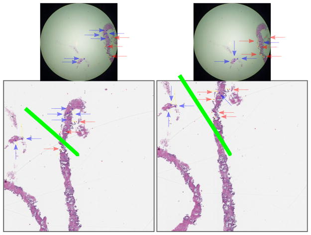
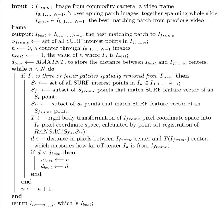
The partially automated registration process starts with initial manual registration of a frame, followed by automated registration within the preceding registration’s spatial neighborhood (Fig 4 and Alg 1). First, (i) a set Sframe of SURF interest points were found in the video frame, (ii) a set St of SURF interest points were found in a slide image patch, (iii) SURF interest point feature vectors were compared in Sframe and St to determine which points were shared in Sframe and St, and (iv) subsets of Sframe and St points that were shared were then stored in Sfs and Sts, respectively. Points shared between a camera video frame and an image patch (Fig 4 at left, top and bottom) change depending on the image patch (Fig 4 at right, top and bottom). Second, we used the OpenCV implementation of random sample consensus [RANSAC] [11] for point set registration, to calculate a rigid body transformation from Sfs point pixel positions in the video frame to Sts point pixel positions in the image patch, to find the distance in pixels that the video frame is off-center from the patch. Following this procedure for every image patch in the spatial neighborhood of the previous image registration, we selected the least off-center image patch as the best registration, because the pathologist’s fovea is in approximately the same place in this video frame and image patch. Finally, a manual curation of registrations ensures correctness. Because slide movements are usually slight, this automated process reduces manual curation effort because automatic registrations are rarely far from the correct registration, so after the registration is corrected within a small localized neighborhood, automatic registrations may proceed from there. Fully automated image registration is not part of this study.
Fig. 4.
The best image registration for a given video frame (same frame top left and top right) from the commodity camera at the microscope eyepiece compared to two different high-quality patches (bottom left and bottom right) from the whole slide scan image minimizes the length of the green line, which is the distance from the center of the patch to the center of the frame mapped into the patch’s coordinate space. The green line’s length is distance d in Alg 1.
Algorithm 1.
Automated image registration procedure (Fig 4) to find the least off-center patch from a given commodity camera video frame. The whole slide image is split into N overlapping 800 × 800 px patches. “Three or fewer patches spatially removed” means any In must be (i) Iprior, (ii) adjacent to Iprior, (iii) adjacent to a patch adjacent to Iprior, or (iv) adjacent to a patch adjacent to an Iprior-adjacent patch. In this way, In is restricted to a spatial neighborhood localized around the prior match, typically improving image registration performance because most slide movements are small. On lens change, (i) the patch at lower magnification and (ii) the patches at higher magnification covering the same area as the current magnification’s neighborhood are considered for registration only.
Slide magnification may change during inspection as the pathologist changes objective lenses. Lens change is detected automatically when the field of view bounding box of nonblack pixels changes size (Fig 5). SURF is scale-invariant so registrations may otherwise proceed at an unchanged magnification.
Fig. 5.
Lens change detection: the normal non-black pixel bounding box is initially 415×415 px. A change to 415×282 px indicates the pathologist changing the lens, thus changing slide magnification. Note some pixels that may appear black are called non-black due to difficult to perceive noise in the image, which effects calculated bounding box size. All images shown at same scale trimmed to bounding box.
Deep learning
We used Caffe [14] for deep learning of convolutional features in a binary classification model given the 800 × 800 px image patches labeled with pathologist viewing times in seconds. To adapt for our purpose CaffeNet (Fig 6), which is similar to AlexNet [17], we re-initialized its top layer’s weights after ImageNet [6] pre-training. Two output neurons were connected to the reinitialized layer, then training followed on augmented 800 × 800 px patches for 10,000 iterations in Caffe. In bladder, our model simply predicted whether or not a pathologist viewed an 800×800 px patch more than 0.1 s (30 fps camera). In prostate, due to the higher overlap between adjacent patches and less tissue available, to be salient a patch met at least one of these criteria: (1) viewed more than 0.1 s, (2) immediately above, below, left, or right of at least two patches viewed more than 0.1 s, or (3) above, below, left, right, or diagonal from at least three patches viewed more than 0.1 s such that all three are not on the same side. In this way, image patches highly overlapping in the neighborhood (Alg 1) of salient patches were not themselves considered non-salient if a pathologist happened to jump over them during observation.
Fig. 6.
Caffenet neuron counts, convolutional layers, pooling layers, dropout [26] layers, and fully-connected layers.
3 Experiments
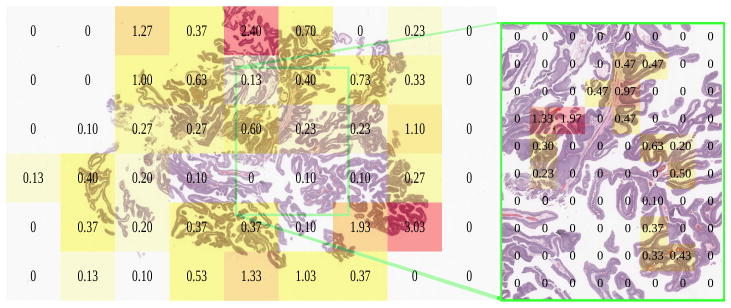
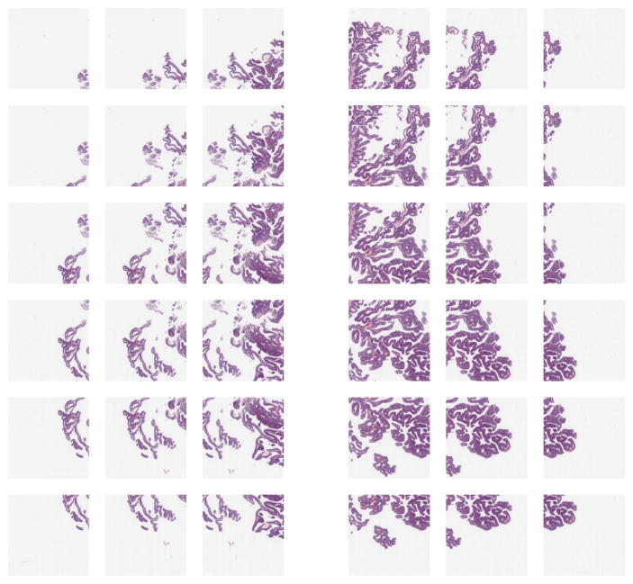
Urothelial carcinoma (bladder) in Fig 7 was analyzed first, with author HAA inspecting at the microscope. Viewed regions at the microscope corresponded to the whole-slide scan SVS file at magnification levels 2 and 1. We restricted our analysis to level 2, having insufficient level 1 data. We split level 2 into three portions: left, center, and right. Due to over 50% overlap among the slide’s total 54 800 × 800 px level 2 patches, we excluded the center portion from analysis, but retained left and right sides, which did not overlap (Fig 8).
Fig. 7.
Pathologist viewing times in seconds at the microscope for low (left, 10x, level 2) and high magnification (right, 20x, level 1), registered to the same urothelial carcinoma slide scan.
Fig. 8.
Scaled image patches of left and right sides of bladder patient 1 slide (Fig 2). Middle excluded here and not used in analysis, to isolate left and right sides from each other. Note far left and far right have less tissue, but tissue is present for training. The overlap among patches is evenly distributed and greater than 50%.
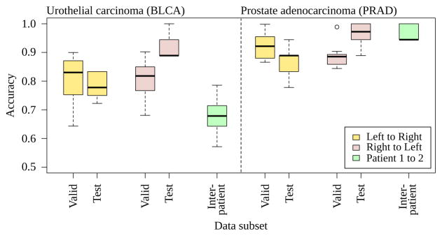
In bladder, we considered a negative example to be a patch viewed for 0.1 s (3 frames or fewer, 30 fps) or less, and a positive example viewed for more than 0.1 s (4 frames or more). This produced 9 positive and 9 negative examples on the left side, and the same number on the right. We performed three-fold cross-validation on the left (6+ and 6− examples training set, 3+ and 3− examples validation set), then used the model with the highest validation accuracy on the right to calculate test accuracy, an estimate of generalization error (Fig 9). This cross-validation was duplicated ten times on the left, each time estimating test accuracy, to calculate a confidence interval. We then duplicated this training/validating on the left and testing on the right.
Fig. 9.
Ten three-fold cross-validation trials for bladder [BLCA] and prostate [PRAD], evaluated for intrapatient training/validating on left while testing on the right and vice versa. Each model is evaluated against a different patient (interpatient), slides in Fig 2). The needle for prostate cancer biopsy may standardize the distribution of prostate tissue in the whole slide, maintaining a higher accuracy of the prostate classifier on an interpatient basis than the bladder cancer classifier. The bladder patients are transurethral resections taken by cuts rather than a standard gauge needle.
Training and validation data were augmented. For a 800 × 800 px patch, all flips and one-degree rotations through 360 degrees were saved, then cropped to the centermost 512×512 px, then scaled to 256×256 px. This rotation-based data augmentation biases the neural network to learn rotationally-invariant features rather than overfit to the training data’s particular orientation, e.g. the angle of prostate needle biopsy tissue strips. Thus intrapatient and interpatient test sets are not augmented, but training and validation sets are augmented. The cancer diagnosis or viewing time in pathology is not expected to change when rotating or flipping a slide. We direct readers to Krizhevsky et al. 2012 [17] for more information on data augmentation. Like Krizhevsky’s data augmentation of 224 × 224 px random crops for small translations, we further augment our dataset through random crops of 227×227 px, which is the default for CaffeNet. Unlike Krizhevsky, we do not augment our dataset through minor perturbations in the principal components of the RGB color space.
In bladder, the augmented training set size was 8,640 patches. This 8,640 count includes rotations and flips, but does not include random crops, which were performed automatically by Caffe at training time. Caffe randomly cropped 256×256 px patches to 227×227 px for each iteration of CaffeNet learning. No images in the validation set were derived from the training set, and vice versa. A training set consists of two concatenated folds, with the remaining fold as validation. In addition to the bladder cancer slide, we analogously processed two prostate cancer needle biopsy slides, with author SJS inspecting these slides. In prostate, the augmented training set size was 8,160 patches.
Training and validation sets are drawn from the same side of the slide, i.e. both sets on the left or both sets on the right (Fig 8). Patches in a training set may have at least 50% overlap with patches in a validation set. Overlapping regions of these images have identical sets of pixels, guaranteeing training and validation sets are exchangeable for valid cross-validation. If training error steadily decreases while validation error steadily increases, where training and validation sets are exchangeable, then the classifier is overfit. In contrast, the other side of the slide is used as a test set and may appear obviously different than the training and validation sets, e.g. the left side of Fig 8 appears different than the right side. We test the other side to estimate generalization error, which measures how the classifier may perform on data unseen at training time. Testing on the other side of the slide guarantees there is no overlap with the training set, so the test data is unseen by the classifier at training time.
Different cross-validation schemes are conceivable, such as (i) a top versus bottom split rather than a left versus right split or (ii) a leave-one-out [LOO] cross-validation approach. Unfortunately, Fig 8 shows a slight overlap in the row second from the top and the row second from the bottom, effectively reducing by 25–50% the amount of data for training, validation, and testing compared to our left versus right approach. Separately, in a LOO setting, one may draw a test patch, then draw training and validation sets randomly that do not overlap with the test patch, keeping training and validation set sizes constant for every possible test patch in the slide. Unfavorably, if the test patch is drawn from the middle column of the slide, then only the leftmost and rightmost columns of patches do not overlap with the test patch, reducing the amount of data for training and validation sets by 33% compared to our left versus right approach. This 33% reduction for middle test patches is in contrast to the 111% increase in training and validation data quantity for test patches drawn from the corners of the leftmost or rightmost columns, where this excess is randomly discarded to maintain constant training and validation set sizes for all possible test patches. Moreover, if the test patch is in the bottom row on the right side, the top row on the right side may be sampled for training, which may inflate the LOO generalization accuracy estimate compared to our cross-validation approach that trains only on the left when testing on the right, due to patches on the right appearing similar to one another. We show in Section 4 that training on the left and testing on the right gives significantly different accuracy compared to training on the right and testing on the left, suggesting the left and right sides have indeed different distributions of information. Thus compared to these alternatives, our left versus right three-fold cross-validation approach (i) maximizes the sizes of the training, validation, and test sets, (ii) conservatively estimates generalization error by not training the classifier on data that appear similar to the test set, and (iii) samples each patch on the left or right sides exactly once for an overall validation error measure for that side.
4 Results
In bladder, when training/validating on the left side and testing on the right, mean test accuracy is 0.781±0.0423 (stdev) with 95% confidence interval [CI] from 0.750 to 0.811 (df=9, Student’s T, Table 1). When training/validating on the right and testing on the left, mean test accuracy is 0.922±0.0468 with 0.889–0.956 95% CI (Table 1). Overall mean test accuracy is 85.15%. The left and right test accuracies differ (p=0.000135, Wilcoxon rank-sum, n=20), while validation accuracies do not (p=0.9118, n=20). This suggests nonhomogenous information content throughout the slide. Indeed, the pathologist started and ended slide inspection on the right, and spent double the time on the right versus the left (Fig 7, 8.32 s right, 4.07 s left). The second bladder had different morphology and model accuracy reduced to 0.678±0.0772, 0.623–0.734 95% CI. Moreover, the second bladder had only 7 positive examples available, whereas both prostates and the first bladder had at least 9 positive examples.
Table 1.
Accuracies of ten trials of three-fold cross-validation in bladder. Validation and test accuracies for a single slide video of urothelial carcinoma (patient 1, slide at upper left in Fig 2, performance plotted at left in Fig 9)), left side of the slide versus right side.
| Direction | Trial | Fold0 Valid | Fold1 Valid | Fold2 Valid | Valid Acc | Fold0 Test | Fold1 Test | Fold2 Test | Test Acc |
|---|---|---|---|---|---|---|---|---|---|
| leftright | 0 | 0.9466 | 0.5850 | 0.9680 | 0.8332 | 0.8333 | 0.7222 | 0.7778 | 0.7778 |
| leftright | 1 | 0.8852 | 0.9070 | 0.9070 | 0.8997 | 0.7778 | 0.7222 | 0.7778 | 0.7500 |
| leftright | 2 | 0.9218 | 0.8602 | 0.8832 | 0.8884 | 0.8333 | 0.7222 | 0.7778 | 0.8333 |
| leftright | 3 | 0.7640 | 0.7812 | 0.7120 | 0.7524 | 0.7778 | 0.7778 | 0.7778 | 0.7778 |
| leftright | 4 | 0.7590 | 0.6576 | 0.5134 | 0.6433 | 0.8333 | 0.7778 | 0.7778 | 0.8333 |
| leftright | 5 | 0.9268 | 0.7416 | 0.5088 | 0.7257 | 0.8333 | 0.7778 | 0.7778 | 0.8333 |
| leftright | 6 | 0.8028 | 0.7988 | 0.7048 | 0.7688 | 0.7222 | 0.7778 | 0.7778 | 0.7222 |
| leftright | 7 | 0.7318 | 0.8402 | 0.9088 | 0.8269 | 0.7778 | 0.7778 | 0.7778 | 0.7778 |
| leftright | 8 | 0.9572 | 0.7608 | 0.8418 | 0.8533 | 0.7778 | 0.8333 | 0.8333 | 0.7778 |
| leftright | 9 | 0.7492 | 0.8774 | 0.9860 | 0.8709 | 0.7778 | 0.7778 | 0.7222 | 0.7222 |
| rightleft | 0 | 0.8802 | 0.8528 | 0.8554 | 0.8628 | 1.0000 | 0.8889 | 0.9444 | 1.0000 |
| rightleft | 1 | 0.7662 | 0.5982 | 0.9364 | 0.7669 | 0.8889 | 0.9444 | 1.0000 | 1.0000 |
| rightleft | 2 | 0.9492 | 0.8560 | 0.7308 | 0.8453 | 0.9444 | 0.8889 | 0.9444 | 0.9444 |
| rightleft | 3 | 0.5404 | 0.8206 | 0.8368 | 0.7326 | 0.9444 | 0.9444 | 0.8889 | 0.8889 |
| rightleft | 4 | 0.6560 | 0.7114 | 0.6748 | 0.6807 | 0.8889 | 0.8889 | 0.8333 | 0.8889 |
| rightleft | 5 | 0.8932 | 0.7062 | 0.7310 | 0.7768 | 0.9444 | 0.8889 | 0.8333 | 0.9444 |
| rightleft | 6 | 0.8560 | 0.8540 | 0.9966 | 0.9022 | 0.8889 | 0.9444 | 0.8889 | 0.8889 |
| rightleft | 7 | 0.8362 | 0.8560 | 0.7978 | 0.8300 | 0.8333 | 0.8889 | 1.0000 | 0.8889 |
| rightleft | 8 | 0.7200 | 0.8546 | 0.9740 | 0.8495 | 1.0000 | 0.9444 | 0.8889 | 0.8889 |
| rightleft | 9 | 0.8634 | 0.8634 | 0.6904 | 0.8057 | 0.8333 | 0.9444 | 1.0000 | 0.8889 |
Column “Fold0 Valid” reports validation accuracy when folds 1 and 2 were used for training. Similarly, “Fold1 Valid” is for folds 0 and 2 training. “Valid Acc” is the validation accuracy overall – the average of “Fold0 Valid”, “Fold1 Valid”, and “Fold2 Valid”. Because we will use a single classifier for saliency prediction, we selected the classifier with highest validation accuracy and highlighted it yellow, e.g. we selected the Fold0 classifier with 0.9218 validation error as shown in the third row, namely Trial 2 leftright.
Column “Fold0 Test” reports the test accuracy of the classifier trained on folds 1 and 2. Because we will use a single classifier not an ensemble, we highlight the test accuracy of the classifier selected by highest validation accuracy and report this in “Test Acc“ as generalization accuracy, e.g. we selected the Trial 2 leftright Fold0 classifier having “Fold0 Test” of 0.8333 and copied this to “Test Acc”. We report test accuracies for all three classifiers, showing Fold1 and Fold2 classifiers tie for highest validation accuracy in Trial 1 leftright, so their test accuracies of 0.7222 and 0.7778 were averaged for a “Test Acc” of 0.7500. As another sanity check in our small data setting, we report that the variance in the selected-versus-non-selected test accuracy differences is not greater than the selected-versus-non-selected validation accuracy differences (F-Test p=0.5662 and Bartlett’s Test p=0.5661. Validation differences normally distributed by Anderson-Darling p=0.08837, and test differences by p=0.1734). If it were greater, there may be experimental setup problems because training would not be stably producing classifiers that learn the saliency concept. Finally, one may train a classifier on all folds then evaluate test accuracy with this classifier, but a performance boost from additional training data may inflate generalization accuracy. In Sec 4 we show without such inflation there remains a significant difference in generalization accuracy and interpatient accuracy in bladder.
Testing the best classifier (highlighted in cyan, highest test accuracy on this and other folds, secondarily highest mean validation accuracy) on draws of the data on the second bladder patient, accuracies are 0.643, 0.786, 0.714, 0.786, 0.714, 0.714, 0.643, 0.571, 0.643, and 0.571.
For the first prostate slide, training on the left side and testing on the right, we find accuracy 0.867±0.0597, 0.824–0.909 95% CI (Table 2). Training on the right and testing on left, we find 0.961±0.0457, 0.928–0.994 95% CI (Table 2). Overall mean test accuracy is 91.40%. Taking the best model learned from this first prostate (right side, test accuracy 100%, 18/18), we tested on the second prostate’s right side (because the left did not have 9 positive training examples) and find 0.967±0.0287, 0.946–0.987 95% CI. We also tested this model on the bladder cancer slide, and find 0.780 accuracy on the left and 0.720 on the right (9+ and 9− training examples each), mean accuracy 75.00%. The best bladder cancer model predicts every patch is not salient in both prostates, presumably because the little tissue in prostate is insufficient for a positive saliency prediction.
Table 2.
Accuracies of ten trials of three-fold cross-validation in prostate. Validation and test accuracies for a single slide video of prostate adenocarcinoma (patient 1, slide at upper right in Fig 2, performance plotted at right in Fig 9)), left side of the slide versus right side.
Testing the best classifier on draws of the data on the second prostate patient, accuracies are 0.944, 1, 0.944, 0.944, 1, 0.944, 0.944, 0.944, 1, and 1.
| Direction | Trial | Fold0 Valid | Fold1 Valid | Fold2 Valid | Valid Acc | Fold0 Test | Fold1 Test | Fold2 Test | Test Acc |
|---|---|---|---|---|---|---|---|---|---|
| leftright | 0 | 0.9992 | 0.9946 | 1.0000 | 0.9979 | 0.7778 | 0.7778 | 0.7778 | 0.7778 |
| leftright | 1 | 0.9512 | 0.7282 | 0.9994 | 0.8929 | 0.8889 | 0.8889 | 0.8889 | 0.8889 |
| leftright | 2 | 0.9550 | 1.0000 | 0.6530 | 0.8693 | 0.8889 | 0.7778 | 0.7222 | 0.7778 |
| leftright | 3 | 0.8636 | 0.9992 | 1.0000 | 0.9543 | 0.8889 | 0.7778 | 0.9444 | 0.9444 |
| leftright | 4 | 0.8276 | 0.7760 | 0.9940 | 0.8659 | 0.8889 | 0.7778 | 0.8889 | 0.8889 |
| leftright | 5 | 0.8654 | 0.9986 | 1.0000 | 0.9547 | 0.9444 | 0.9444 | 0.9444 | 0.9444 |
| leftright | 6 | 0.8560 | 0.9862 | 0.9992 | 0.9471 | 0.8889 | 0.8889 | 0.8889 | 0.8889 |
| leftright | 7 | 0.8674 | 1.0000 | 0.9984 | 0.9553 | 0.8889 | 0.8333 | 0.8889 | 0.8333 |
| leftright | 8 | 0.9560 | 0.8560 | 0.8760 | 0.8960 | 0.8889 | 0.8333 | 0.9444 | 0.8889 |
| leftright | 9 | 0.6846 | 0.9992 | 0.9560 | 0.8799 | 0.8333 | 0.8333 | 1.0000 | 0.8333 |
| rightleft | 0 | 0.9786 | 0.7760 | 0.9146 | 0.8897 | 0.8889 | 0.9444 | 1.0000 | 0.8889 |
| rightleft | 1 | 1.0000 | 0.7292 | 0.8460 | 0.8584 | 1.0000 | 0.9444 | 1.0000 | 1.0000 |
| rightleft | 2 | 0.7130 | 0.9512 | 0.8676 | 0.8439 | 0.8889 | 1.0000 | 0.8333 | 1.0000 |
| rightleft | 3 | 0.9998 | 1.0000 | 0.9664 | 0.9887 | 0.9444 | 0.9444 | 1.0000 | 0.9444 |
| rightleft | 4 | 0.7760 | 1.0000 | 0.8842 | 0.8867 | 0.8889 | 0.9444 | 1.0000 | 0.9444 |
| rightleft | 5 | 0.9758 | 0.9984 | 0.5926 | 0.8556 | 0.9444 | 0.8889 | 0.9444 | 0.8889 |
| rightleft | 6 | 0.6344 | 0.9770 | 1.0000 | 0.8705 | 0.8889 | 1.0000 | 1.0000 | 1.0000 |
| rightleft | 7 | 0.7760 | 0.9028 | 1.0000 | 0.8929 | 0.8889 | 1.0000 | 1.0000 | 1.0000 |
| rightleft | 8 | 0.8560 | 0.8560 | 0.9992 | 0.9037 | 0.9444 | 0.9444 | 0.9444 | 0.9444 |
| rightleft | 9 | 0.8560 | 0.9412 | 0.8538 | 0.8837 | 1.0000 | 1.0000 | 1.0000 | 1.0000 |
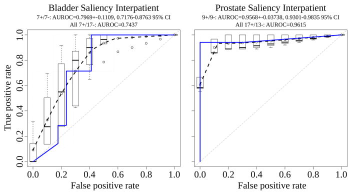
Interpatient AUROC for bladder and prostate is shown in Fig 10. In prostate, nine salient and nine nonsalient examples are drawn from the second patient. Average AUROC was calculated from ten such draws, achieving a mean±stdev of 0.9568±0.0374 and 95% CI of 0.9301–0.9835. Over all 17 salient and 13 nonsalient patches used from the second prostate patient, the AUROC is 0.9615. In bladder, due to fewer patches available in the small slide, only seven salient and seven nonsalient examples are drawn from the second patient. Average AUROC was calculated for ten such draws, achieving 0.7929±0.1109 and 95% CI of 0.7176–0.8763. Over all 7 salient and 17 nonsalient patches used from the second bladder patient, the AUROC is 0.7437. These nonoverlapping confidence intervals are evidence the bladder cancer classifier distinguishes salient from nonsalient patches less well than the prostate cancer classifier, and a Wilcoxon rank-sum test indeed finds the difference in classifier performance by these ten draws each from bladder and prostate is significant (p=0.0001325) (Fig 9).
Fig. 10.
Interpatient area under the receiver operating characteristic [AUROC] for bladder and prostate, with dashed black curve for average AUROC over draws of the data and blue line for all data used from the patient.
The deep convolutional network CaffeNet emits a score from 0 to 1 when predicting if an image patch is salient or not. When taking a score of greater than 0.5 to be salient, the p-value from Fisher’s Exact Test is 1.167e-7 in prostate (16 true positives, 1 false negative, 0 false positives, 13 true negatives) and 0.009916 in bladder (7 true positives, 0 false negatives, 7 false positives, 10 true negatives), indicating our trained CaffeNet classifier in both tissues accurately distinguishes salient from nonsalient regions when trained on one patient and predicting in another.
5 Conclusion
Collecting image-based expert annotations for the deluge of medical data at modern hospitals is one of the tightest bottlenecks for the application of large-scale supervised machine learning. We address this with a novel framework that combines a commodity camera, 3D-printed mount, and software stack to build a predictive model for saliency on whole slides, i.e. where a pathologist looks to make a diagnosis. The registered regions from the digital slide scan are markedly higher quality than the camera frames, since they do not suffer from debris, vignetting, and other artifacts. The proposed CNN is able to predict salient slide regions with a test accuracy of 85–91%. We plan to scale up this pilot study to more patients, tissues, and pathologists.
Acknowledgments
AJS was supported by NIH/NCI grant F31CA214029 and the Tri-Institutional Training Program in Computational Biology and Medicine (via NIH training grant T32GM083937). This research was funded in part through the NIH/NCI Cancer Center Support Grant P30CA008748. AJS thanks Terrie Wheeler, Du Cheng, and the Medical Student Executive Committee of Weill Cornell Medical College for free 3D printing access, instruction, and support. AJS thanks Mariam Aly for taking the photo of the camera on the orange 3D-printed mount in Fig 1, and attention discussion. We acknowledge fair use of part of a doctor stick figure image in Fig 1 from 123rf.com. AJS thanks Mark Rubin for helpful pathology discussion. AJS thanks Paul Tatarsky and Juan Perin for Caffe install help on the Memorial Sloan Kettering supercomputer. We gratefully acknowledge NVIDIA Corporation for providing us a GPU as part of the GPU Research Center award to TJF, and for their support with other GPUs.
Footnotes
ImageJ SURF is released under the GNU GPL and is available for download from http://labun.com/imagej-surf/
References
- 1.Ball R, North C. The effects of peripheral vision and physical navigation on large scale visualization. Proceedings of Graphics Interface. 2008;2008:9–16. [Google Scholar]
- 2.Ball R, North C, Bowman D. Move to Improve: Promoting Physical Navigation to Increase User Performance with Large Displays. ACM; 2007. pp. 191–200. [Google Scholar]
- 3.Bay H, Tuytelaars T, Van Gool L. SURF: Speeded Up Robust Features. In: Leonardis A, Bischof H, Pinz A, editors. Computer Vision – ECCV 2006. Vol. 3951. Springer; Berlin Heidelberg: 2006. pp. 404–417. [DOI] [Google Scholar]
- 4.Begelman G, Lifshits M, Rivlin E. Visual positioning of previously defined ROIs on microscopic slides. IEEE Transactions on Information Technology in Biomedicine. 2006 Jan;10(1):42–50. doi: 10.1109/titb.2005.856856. [DOI] [PubMed] [Google Scholar]
- 5.Brunye T, Carney P, Allison K, Shapiro L, Weaver D, Elmore J. Eye Movements as an Index of Pathologist Visual Expertise: A Pilot Study. PLoS ONE. 2014 Aug;9(8):e103447. doi: 10.1371/journal.pone.0103447. [DOI] [PMC free article] [PubMed] [Google Scholar]
- 6.Deng J, Dong W, Socher R, Li LJ, Li K, Fei-Fei L. ImageNet: A large-scale hierarchical image database. IEEE; Jun, 2009. pp. 248–255. [Google Scholar]
- 7.Eivazi S, Bednarik R, Leinonen V, von und zu Fraunberg Mikael, Jaaskelainen J. Embedding an Eye Tracker Into a Surgical Microscope: Requirements, Design, and Implementation. IEEE Sensors Journal. 2016 Apr;16(7):2070–2078. [Google Scholar]
- 8.Erwin D. The Interface of Language, Vision, and Action. Routledge; Jun, 2004. The Interface of Language, Vision, and Action. [DOI] [Google Scholar]
- 9.Farneback G. PhD thesis. Linkoping University; Sweden: 2002. Polynomial Expansion for Orientation and Motion Estimation. [Google Scholar]
- 10.Farneback G. Two-frame Motion Estimation Based on Polynomial Expansion. Springer-Verlag; 2003. pp. 363–370. [Google Scholar]
- 11.Fischler M, Bolles R. Random sample consensus: a paradigm for model fitting with applications to image analysis and automated cartography. Communications of the ACM. 1981 Jun;24(6):381–395. [Google Scholar]
- 12.Fuchs T, Buhmann J. Computational pathology: challenges and promises for tissue analysis. Computerized medical imaging and graphics : the official journal of the Computerized Medical Imaging Society. 2011 Oct;35(7–8):515–530. doi: 10.1016/j.compmedimag.2011.02.006. [DOI] [PubMed] [Google Scholar]
- 13.Goode A, Gilbert B, Harkes J, Jukic D, Satyanarayanan M. OpenSlide: A vendor-neutral software foundation for digital pathology. Journal of pathology informatics. 2013;4 doi: 10.4103/2153-3539.119005. [DOI] [PMC free article] [PubMed] [Google Scholar]
- 14.Jia Y, Shelhamer E, Donahue J, Karayev S, Long J, Girshick R, Guadarrama S, Darrell T. Caffe: Convolutional Architecture for Fast Feature Embedding. 2014 Jun; [Google Scholar]
- 15.Just M, Carpenter P. A theory of reading: From eye fixations to comprehension. Psychological Review. 1980;87(4):329–354. [PubMed] [Google Scholar]
- 16.Keerativittayanun S, Rakjaeng K, Kondo T, Kongprawechnon W, Tungpimolrut K, Leelasawassuk T. Eye tracking system for Ophthalmic Operating Microscope. IEEE; Aug, 2009. pp. 653–656. [Google Scholar]
- 17.Krizhevsky A, Sutskever I, Hinton G. Imagenet classification with deep convolutional neural networks. 2012 [Google Scholar]
- 18.Krupinski E, Tillack A, Richter L, Henderson J, Bhattacharyya A, Scott K, Graham A, Descour M, Davis J, Weinstein R. Eye-movement study and human performance using telepathology virtual slides. Implications for medical education and differences with experience. Human Pathology. 2006 Dec;37(12):1543–1556. doi: 10.1016/j.humpath.2006.08.024. [DOI] [PubMed] [Google Scholar]
- 19.Mercan E, Aksoy S, Shapiro L, Weaver D, Brunye T, Elmore J. Localization of Diagnostically Relevant Regions of Interest in Whole Slide Images. IEEE; Aug, 2014. pp. 1179–1184. [DOI] [PMC free article] [PubMed] [Google Scholar]
- 20.Parwani A, Hassell L, Glassy E, Pantanowitz L. Regulatory barriers surrounding the use of whole slide imaging in the United States of America. Journal of pathology informatics. 2014;5(1) doi: 10.4103/2153-3539.143325. [DOI] [PMC free article] [PubMed] [Google Scholar]
- 21.Raghunath V, Braxton M, Gagnon S, Brunye T, Allison K, Reisch L, Weaver D, Elmore J, Shapiro L. Mouse cursor movement and eye tracking data as an indicator of pathologists’ attention when viewing digital whole slide images. Journal of pathology informatics. 2012;3 doi: 10.4103/2153-3539.104905. [DOI] [PMC free article] [PubMed] [Google Scholar]
- 22.Randell R, Ambepitiya T, Mello-Thoms C, Ruddle R, Brettle D, Thomas R, Treanor D. Effect of Display Resolution on Time to Diagnosis with Virtual Pathology Slides in a Systematic Search Task. Journal of Digital Imaging. 2015;28(1):68–76. doi: 10.1007/s10278-014-9726-8. [DOI] [PMC free article] [PubMed] [Google Scholar]
- 23.Romo D, Romero E, Gonzalez F. Learning regions of interest from low level maps in virtual microscopy. Diagnostic Pathology. 2011;6(Suppl 1):S22. doi: 10.1186/1746-1596-6-S1-S22. [DOI] [PMC free article] [PubMed] [Google Scholar]
- 24.Schneider C, Rasband W, Eliceiri K. NIH Image to ImageJ: 25 years of image analysis. Nature methods. 2012 Jul;9(7):671–675. doi: 10.1038/nmeth.2089. [DOI] [PMC free article] [PubMed] [Google Scholar]
- 25.Shupp L, Ball R, Yost B, Booker J, North C. Evaluation of viewport size and curvature of large, high-resolution displays. Canadian Information Processing Society; 2006. pp. 123–130. [Google Scholar]
- 26.Srivastava N, Hinton G, Krizhevsky A, Sutskever I, Salakhutdinov R. Dropout: A Simple Way to Prevent Neural Networks from Overfitting. 2014 Jun;15:1929–1958. [Google Scholar]
- 27.Starkweather G. 58.4: DSHARP — A Wide Screen Multi-Projector Display. SID Symposium Digest of Technical Papers. 2003 May;34(1):1535–1537. [Google Scholar]


