

Abstract
A novel Gaussian Accelerated Molecular Dynamics (GaMD) method has been developed for simultaneous unconstrained enhanced sampling and free energy calculation of biomolecules. Without the need to set predefined reaction coordinates, GaMD enables unconstrained enhanced sampling of the biomolecules. Furthermore, by constructing a boost potential that follows a Gaussian distribution, accurate reweighting of GaMD simulations is achieved via cumulant expansion to the second order. The free energy profiles obtained from GaMD simulations allow us to identify distinct low energy states of the biomolecules and characterize biomolecular structural dynamics quantitatively. In this chapter, we present the theory of GaMD, its implementation in the widely used molecular dynamics software packages (AMBER and NAMD), and applications to the alanine dipeptide biomolecular model system, protein folding, biomolecular large-scale conformational transitions and biomolecular recognition.
Keywords: Gaussian Accelerated Molecular Dynamics, Biomolecules, Enhanced Sampling, Free Energy, Protein Folding, Conformational Transitions, Biomolecular Recognition, Ligand Binding
1 Introduction
Biomolecules such as proteins, lipids and nucleic acids often undergo structural changes between different low-energy conformational states. The structural dynamics of biomolecules plays an essential role in their biological function, e.g., gene translation/editing, protein folding, biomolecular recognition and cellular signaling1, 2, 3, 4. The structure, dynamics and function of biomolecules have been suggested to result from the underlying free energy landscapes5, 6. It is important to calculate free energy profiles of biomolecules in order to understand their functional mechanisms. However, conformational transitions of biomolecules usually take place on timescales of milliseconds or even longer, due to high-energy barriers (e.g., 8-12 kcal/mol)1, 7, 8. Sufficient conformational sampling and accurate free energy calculations have proven challenging for computational molecular dynamics (MD) simulations that are limited to typically hundreds-of-nanoseconds to tens of microseconds9, 10, 11, 12.
To address this challenge, biasing simulation methods have been found to be useful in enhanced sampling and free energy calculations of biomolecules. These methods include umbrella sampling13, 14, conformational flooding15, 16, metadynamics17, 18, adaptive biasing force (ABF) calculations19, 20, orthogonal space sampling21, 22, etc. During the simulations, a potential or force bias is applied along certain reaction coordinates (or collective variables) to facilitate the biomolecular conformational transitions across high-energy barriers. Typical reaction coordinates include atom distances, torsional dihedrals, root-mean square deviation (RMSD) relative to a reference configuration, eigenvectors generated from the principal component analysis16, and so on. The definition of the reaction coordinates, however, often requires expert knowledge of the studied systems. Furthermore, the pre-defined reaction coordinates largely place constraints on the pathway and conformational space to be sampled during the biasing simulations, which often leads to slow convergence of the simulations when important reaction coordinates are missed during the simulation setup18.
Accelerated molecular dynamics (aMD)23, 24 is an enhanced sampling technique that works often by adding a non-negative boost potential to smooth the system potential energy surface. The boost potential, ΔV decreases the energy barriers and thus accelerates transitions between the different low-energy states24, 25. With this, aMD is able to sample distinct biomolecular conformations and rare barrier-crossing events that are not accessible to conventional MD (cMD) simulations. Unlike the above-mentioned biasing simulation methods, aMD does not require pre-defined reaction coordinate(s), which can be advantageous for exploring the biomolecular conformational space without a priori knowledge or restraints. aMD has been successfully applied to a number of biological systems26, 27, 28, 29, 30 and hundreds-of-nanoseconds aMD simulations have been shown to capture millisecond-timescale events in both globular and membrane proteins31, 32, 33.
Whereas aMD has been demonstrated to greatly enhance the conformational sampling of biomolecules, it suffers from large energetic noise during reweighting34. The boost potential applied in aMD simulations is typically on the order of tens to hundreds of kcal/mol, which is much greater in magnitude and wider in distribution than that of other biasing simulation methods that make use of pre-defined reaction coordinates (e.g., several kcal/mol). It has been a long-standing problem to accurately reweight aMD simulations and recover the original free energy landscapes, especially for large proteins35, 36. Our recent studies showed that when the boost potential follows near-Gaussian distribution, cumulant expansion to the second order provides improved reweighting of aMD simulations compared with the previously used exponential average and Maclaurin series expansion reweighting methods37. The reweighted free energy profiles are in good agreement with the long-timescale cMD simulations as demonstrated on alanine dipeptide and fast-folding proteins38. However, such improvement is limited to rather small systems (e.g., proteins with less than ~35 amino acid residues)38. In simulations of larger systems, the boost potential exhibits significantly wider distribution and does not allow for accurate reweighting.
Here, a Gaussian Accelerated Molecular Dynamics (GaMD) approach is presented to reduce the energetic noise for simultaneous unstrained enhanced sampling and free energy calculation of biomolecules, even for large proteins39, 40. GaMD makes use of a harmonic function to construct the boost potential that is adaptively added to the biomolecular potential energy surface. A minimal set of simulation parameters is dynamically adjusted to control the magnitude and distribution width of the boost potential. As such, the resulting boost potential follows a Gaussian distribution and allows for accurate reweighting of the simulations using cumulant expansion to the second order. In this chapter, we present the theory of GaMD, its implementation in widely used molecular dynamics software packages (particularly AMBER41 and NAMD42), and applications to the alanine dipeptide biomolecular model system, protein folding, biomolecular large-scale conformational transitions and biomolecular recognition.
2 Theory
2.1 Gaussian Accelerated Molecular Dynamics (GaMD)
Gaussian Accelerated Molecular Dynamics (GaMD) enhances the conformational sampling of biomolecules by adding a harmonic boost potential to smooth the system potential energy surface (Figure 1)39. Consider a system with N atoms at positions . When the system potential is lower than a threshold energy E, a boost potential is added as:
| (1) |
where k is the harmonic force constant. The modified system potential, is given by:
| (2) |
Otherwise, when the system potential is above the threshold energy, i.e., , the boost potential is set to zero and .
Figure 1.
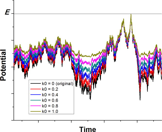
Schematic illustration of Gaussian Accelerated Molecular Dynamics (GaMD): when the threshold energy is set to the maximum potential , the system potential energy surface is smoothed by adding a harmonic boost potential that follows Gaussian distribution. The system original potential energy obtained from conventional molecular dynamics (cMD) is shown in black. The modified potential energy surfaces obtained after adding the boost potential with different effective harmonic constants k0 are shown in red (0.2), blue (0.4), cyan (0.6), purple (0.8) and yellow (1.0). With greater k0, higher boost potential is added to the original energy surface, which provides enhanced sampling of biomolecules across decreased energy barriers.
In order to smooth the potential energy surface for enhanced sampling, the boost potential needs to satisfy the following criteria. First, for any two arbitrary potential values and found on the original energy surface, if , should be a monotonic function that does not change the relative order of the biased potential values, i.e., . By replacing with Equation (2) and isolating E, we then obtain:
| (3) |
Second, if , the potential difference observed on the smoothened energy surface should be smaller than that of the original, i.e., . Similarly, by replacing with Equation (2), we can derive:
| (4) |
With , we need to set the threshold energy E in the following range by combining Equations (3) and (4):
| (5) |
where and are the system minimum and maximum potential energies. To ensure that Equation (5) is valid, and k have to satisfy:
| (6) |
Let us define , then . As illustrated in Figure 1, determines the magnitude of the applied boost potential. With greater , higher boost potential is added to the potential energy surface, which provides enhanced sampling of biomolecules across decreased energy barriers.
Third, the standard deviation of needs to be small enough (i.e., narrow distribution) to ensure accurate reweighting using cumulant expansion to the second order37:
| (7) |
where and are the average and standard deviation of the system potential energies, is the standard deviation of with as a user-specified upper limit (e.g., 10kBT) for accurate reweighting.
Provided Equation (5) that gives the range of threshold energy E, when E is set to the lower bound , we substitute in E and k, and obtain:
| (8) |
Let us define the RHS in Equation (8) as . For efficient enhanced sampling with the highest possible acceleration, can then be set to its upper bound as:
| (9) |
The greater is obtained from the original potential energy surface (particularly for large biomolecules), the smaller may be applicable to allow for accurate reweighting. Alternatively, when the threshold energy E is set to its upper bound according to Equation (5), we substitute in E and k in Equation (7) and obtain:
| (10) |
Let us define the RHS in Equation (10) as . Note that a smaller will give higher threshold energy E, but smaller force constant k. When , can be set to either for the highest threshold energy E or its upper bound 1.0 for the greatest force constant k. In this regard, is applied in the current GaMD. Otherwise, is calculated using Eqn. (9).
Given E and , we can calculate the boost potential as:
| (11) |
Similar to aMD, GaMD provides options to add only the total potential boost , only dihedral potential boost , or the dual potential boost (both and ). The dual-boost simulation generally provides higher acceleration than the other two types of simulations for enhanced sampling25. The simulation parameters comprise of the threshold energy values and the effective harmonic force constants, and for the total and dihedral potential boost, respectively.
2.2 Energetic Reweighting of GaMD for Free Energy Calculations
For simulations of a biomolecular system, the probability distribution along a selected reaction coordinate is written as , where r denotes the atomic positions . Given the boost potential of each frame, can be reweighted to recover the canonical ensemble distribution, , as:
| (12) |
where M is the number of bins, and is the ensemble-averaged Boltzmann factor of for simulation frames found in the jth bin. In order to reduce the energetic noise, the ensemble-averaged reweighting factor can be approximated using cumulant expansion43, 44:
| (13) |
where the first three cumulants are given by:
| (14) |
When the boost potential follows near-Gaussian distribution, cumulant expansion to the second order (or “Gaussian Approximation”) provides the accurate approximation for free energy calculations37. The reweighted free energy is calculated as:
| (15) |
where is the modified free energy obtained from GaMD simulation and is a constant.
To characterize the extent to which ΔV follows Gaussian distribution, its distribution anharmonicity is calculated as37:
| (16) |
where ΔV is dimensionless as divided by with and T being the Boltzmann constant and system temperature, respectively, and is the maximum entropy of ΔV45. When γ is zero, ΔV follows exact Gaussian distribution with sufficient sampling. Reweighting by approximating the exponential average term with cumulant expansion to the second order is able to accurately recover the original free energy landscape. As γ increases, the ΔV distribution becomes less harmonic and the reweighted free energy profile obtained from cumulant expansion to the second order would deviate from the original. The anharmonicity of ΔV distribution serves as an indicator of the enhanced sampling convergence and accuracy of the reweighted free energy. Nevertheless, with the new GaMD theoretical framework, the GaMD boost potential does not change shape of the biomolecular overall energy landscape. A near Gaussian distribution is achieved for the GaMD boost potential.
3 Implementation
3.1 Implementation of GaMD in AMBER
GaMD was originally implemented in the GPU version of AMBER 1246, and was later transferred to AMBER 14 with a patch available. Currently, GaMD is fully supported in AMBER 16 (http://gamd.ucsd.edu). GaMD provides enhanced sampling of biomolecules by adding a harmonic boost potential to smooth the system potential energy surface. Following is a list of the input parameters for a GaMD simulation:
| igamd | Flag to apply boost potential |
| = 0 (default) no boost is applied | |
| = 1 boost on the total potential energy only | |
| = 2 boost on the dihedral energy only | |
| = 3 dual boost on both dihedral and total potential energy | |
| iE | Flag to set the threshold energy E |
| = 1 (default) set the threshold energy to the lower bound E = Vmax | |
| = 2 set the threshold energy to the upper bound E = Vmin + (Vmax - Vmin)/k0 | |
| ntcmd | The number of initial conventional molecular dynamics simulation steps used to calculate the maximum, minimum, average and standard deviation of the system potential energies (i.e., Vmax, Vmin, Vavg, σV). The default is 1,000,000 for a simulation with 2 fs timestep. |
| nteb | The number of simulation steps used to equilibrate the system after adding boost potential. The default is 1,000,000 for a simulation with 2 fs timestep. |
| sigma0P | The upper limit of the standard deviation of the total potential boost that allows for accurate reweighting if igamd is set to 1 or 3. The default is 6.0 (unit: kcal/mol). |
| sigma0D | The upper limit of the standard deviation of the dihedral potential boost that allows for accurate reweighting if igamd is set to 2 or 3. The default is 6.0 (unit: kcal/mol). |
The GaMD algorithm is summarized as the following:
| GaMD { |
| For i = 1, …, ntcmd // run short initial conventional molecular dynamics |
| Calculate Vmax, Vmin, Vavg, sigmaV |
| End |
| Calc_E_k0(iE,sigma0,Vmax,Vmin,Vavg,sigmaV) |
| For i = 1, …, nteb // Equilibrate the system after adding boost potential |
| deltaV = 0.5*k0*(E-V)**2/(Vmax-Vmin) |
| V = V + deltaV |
| Update Vmax, Vmin, Vavg, sigmaV |
| Calc_E_k0(iE,sigma0,Vmax,Vmin,Vavg,sigmaV) |
| End |
| For i = 1, …, nstlim // run production simulation |
| deltaV = 0.5*k0*(E-V)**2/(Vmax-Vmin) |
| V = V + deltaV |
| End |
| } |
| Subroutine Calc_E_k0(iE,sigma0,Vmax,Vmin,Vavg,sigmaV) { |
| if iE = 1 : |
| E = Vmax |
| k0′ = (sigma0/sigmaV) * (Vmax-Vmin)/(Vmax-Vavg) |
| k0 = min(1.0, k0′) |
| else if iE = 2 : |
| k0″ = (1-sigma0/sigmaV) * (Vmax-Vmin)/(Vavg-Vmin) |
| if 0 < k0” <= 1 : |
| k0 = k0” |
| else |
| k0 = 1.0 |
| end |
| E = Vmin + (Vmax-Vmin)/k0 |
| end |
| } |
3.2 Implementation of GaMD in NAMD
GaMD has also been implemented in another popular MD software package NAMD40. Similar to the previous aMD implemented in NAMD47, three modes are available for applying boost potential to biomolecules in GaMD: (1) boosting the dihedral energetic term only, (2) boosting the total potential energy only, and (3) boosting both the dihedral and total potential energetic terms (i.e., “dual-boost”). The major code modification is to extend the aMD function in NAMD 2.11 to include the boost potential calculation used in GaMD. The GaMD boost potential is computed based on statistics of the system potential such as the minimum, maximum, average and standard deviation. Therefore, three stages of simulation are needed to collect the potential statistics. They include the (i) cMD stage, (ii) equilibration and (iii) production stages. The program first collects potential statistics from a short cMD run. Subsequently, a boost potential is added to the system in the equilibration stage while update of the potential statistics continues. During this stage, the boost potential applied in each step is computed based on the energetic statistics collected up to that particular step. After the equilibration stage, the statistics collected is assumed to be sufficient to represent the potential energy landscape of interest. Hence, the potential statistics are fixed to calculate the boost potential for running the production simulation. Note that in both the cMD and equilibration stages, there are a small number of steps at the beginning of each stage during which we do not collect statistics. These steps, named preparation steps, are performed to allow the system to adapt to the simulation environment. The program starts collecting statistics of the potential energies after the preparation steps.
The GaMD algorithm is implemented in NAMD 2.1142 as the following:
| GaMD { |
| If (accelMDGRestart == 1) then |
| Read parameters from restart file |
| Jump to the state written in the restart file |
| End if |
| For i = 1, …, cMDSteps // run short initial conventional molecular dynamics |
| if (i == cMDPrepSteps) reset Vmax, Vmin, Vavg, sigmaV |
| Update_Stat(n,V,Vmax,Vmin,Vavg,M2,sigmaV) |
| if (i % restartfreq) Save restart file |
| End |
| Calc_E_k(iE,sigma0,Vmax,Vmin,Vavg,sigmaV) |
| For i = 1, …, EquilSteps // Equilibrate the system after adding boost potential |
| If (E > V) then |
| deltaV = 0.5*k*(E-V)**2 |
| V = V + deltaV |
| EndIf |
| Update_Stat(n,V,Vmax,Vmin,Vavg,M2,sigmaV) |
| if (i >= EquilPrepSteps) |
| Calc_E_k(iE,sigma0,Vmax,Vmin,Vavg,sigmaV) |
| if (i % restartfreq) Save restart file |
| End |
| For i = 1, …, ProdSteps // run production simulation |
| If (E > V) then |
| deltaV = 0.5*k*(E-V)**2 |
| V = V + deltaV |
| EndIf |
| if (i % restartfreq) Save restart file |
| End |
| } |
| Subroutine Update_Stat(n,V,Vmax,Vmin,Vavg,M2,sigmaV) { |
| if (V > Vmax) Vmax = V |
| if (V < Vmin) Vmin = V |
| Vdiff = V – Vavg |
| Vavg = Vavg + Vdiff / n |
| M2 = M2 + Vdiff * (V – Vavg) |
| sigmaV = sqrt(M2 / n) |
| n = n + 1 |
| } |
| Subroutine Calc_E_k(iE,sigma0,Vmax,Vmin,Vavg,sigmaV) { |
| if iE = 1 : |
| E = Vmax |
| k0′ = (sigma0/sigmaV) * (Vmax-Vmin)/(Vmax-Vavg) |
| k0 = min(1.0, k0′) |
| else if iE = 2 : |
| k0” = (1-sigma0/sigmaV) * (Vmax-Vmin)/(Vavg-Vmin) |
| if 0 < k0” <= 1 : |
| k0 = k0” |
| E = Vmin + (Vmax-Vmin)/k0 |
| else |
| E = Vmax |
| k0′ = (sigma0/sigmaV) * (Vmax-Vmin)/(Vmax-Vavg) |
| k0 = min(1.0, k0′) |
| end |
| end |
| k = k0/(Vmax-Vmin) |
| } |
The following is a list of the input parameters for GaMD simulation in NAMD:
-
-
accelMDG < Is Gaussian accelerated MD on? >
Acceptable Values: on or off
Default Value: off
Description: Specifies whether Gaussian accelerated MD (GaMD) is on.
-
-
accelMDGiE < Flag to set the threshold energy E for adding boost potential >
Acceptable Values: 1, 2
Default Value: 1
Description: Specifies how the threshold energy E is set in GaMD. A value of 1 indicates that the threshold energy E is set to its lower bound E = Vmax. A value of 2 indicates that the threshold energy E is set to its upper bound E = Vmin + (Vmax - Vmin) / k0.
-
-
accelMDGcMDPrepSteps < no. of preparatory cMD steps >
Acceptable Values: Zero or Positive integer
Default Values: 200,000
Description: The number of preparatory conventional MD (cMD) steps in GaMD. This value should be smaller than accelMDGcMDSteps (see below). Potential energies are not collected for calculating the values of Vmax, Vmin, Vavg, σV during the first accelMDGcMDPrepSteps.
-
-
accelMDGcMDSteps < no. of total cMD steps in GaMD >
Acceptable Values: Positive integer
Default Value: 1,000,000
Description: The number of total cMD steps in GaMD. With accelMDGcMDPrepSteps < t < accelMDGcMDSteps, Vmax, Vmin, Vavg, σV are collected and at t = accelMDGcMDSteps, E and k0 are computed.
-
-
accelMDGEquiPrepSteps < no. of preparatory equilibration steps in GaMD >
Acceptable Values: Zero or Positive integer
Default Value: 200,000
Description: The number of preparatory equilibration steps in GaMD. This value should be smaller than accelMDGEquiSteps (see below). With accelMDGcMDSteps < t < accelMDGEquiPrepSteps + accelMDGcMDSteps, GaMD boost potential is applied according to E and k0 obtained at t=accelMDGcMDSteps.
-
-
accelMDGEquiSteps < no. of total equilibration steps in GaMD >
Acceptable Values: Zero or Positive integer
Default Value: 1,000,000
Description: The number of total equilibration steps in GaMD. With accelMDGEquiPrepSteps + accelMDGcMDSteps < t < accelMDGEquiSteps + accelMDGcMDSteps, GaMD boost potential is applied, and E and k0 are updated every step.
-
-
accelMDGSigma0P < upper limit of the standard deviation of the total boost potential in GaMD >
Acceptable Values: Positive real number
Default Value: 6.0 (kcal/mol)
Description: Specifies the upper limit of the standard deviation of the total boost potential. This option is only available when accelMDdihe is off or when accelMDdual is on.
-
-
accelMDGSigma0D < upper limit of S.D. of the dihedral potential boost in GaMD >
Acceptable Values: Positive real number
Default Value: 6.0 (kcal/mol)
Description: Specifies the upper limit of the standard deviation of the dihedral boost potential. This option is only available when accelMDdihe or accelMDdual is on.
-
-
accelMDGRestart < Flag to restart GaMD simulation >
Acceptable Values: on or off
Default Value: off
Description: Specifies whether the current GaMD simulation is the continuation of a previous run. If this option is turned on, the GaMD restart file specified by accelMDGRestartFile (see below) will be read.
-
-
accelMDGRestartFile < Name of GaMD restart file >
Acceptable Values: UNIX filename
Description: A GaMD restart file that stores the current number of steps, maximum, minimum, average, standard deviation of the dihedral and/or total potential energies (depending on the accelMDdihe and accelMDdual parameters) and the current timestep settings. This file is saved automatically every restartfreq steps. If accelMDGRestart is turned on, this file will be read and the simulation will restart from the point where the file was written.
3.3 “PyReweighting” toolkit for Energetic Reweighting
A toolkit of Python scripts “PyReweighting”37 has been developed to reweight the GaMD (as well as aMD) simulations for calculating the potential of mean force (PMF) profiles and examine the boost potential distributions. “PyReweighting” is distributed free of charge at http://mccammon.ucsd.edu/computing/amdReweighting/. In addition to the cumulant expansion to the second order reweighting as described in Section 2.2, “PyReweighting” provides the “exponential average” and Maclaurin series expansion reweighting algorithms for comparison.
In the “exponential average” algorithm, the ensemble-averaged Boltzmann reweighting factor of for simulation frames found in the jth bin in Equation (12) is calculated directly. Because the Boltzmann reweighting factors are often dominated by high boost potential frames, the “exponential average” reweighting leads to high energetic noise for free energy calculations37.
Furthermore, the exponential term can be approximated by summation of the Maclaurin series of boost potential with the reweighting factor rewritten as:
| (17) |
where the subscript j has been suppressed. The Maclaurin series expansion up to the 5th-10th order has been used in practice to reweight aMD trajectories31. The reweighted PMF profiles are typically less noisy than those obtained from exponential average reweighting. Note that the Maclaruin series expansion is equivalent to cumulant expansion on the first order37:
| (18) |
When the boost potential follows near-Gaussian distribution, cumulant expansion to the second order (or “Gaussian Approximation”) provides more accurate reweighting compared with the exponential average and Maclaurin series expansion methods37.
4 Applications
GaMD provides unconstrained enhanced sampling of biomolecules without the need to set predefined reaction coordinates. This enables a wide range of technological applications in biomolecular modeling. Furthermore, the GaMD boost potential follows Gaussian distribution, which allows accurate reweighting using cumulant expansion to the 2nd order and recovery of the original biomolecular free energy landscapes, even for large proteins39, 40, 48. Depending on the system size, GaMD provides orders of magnitude speedup for biomolecular simulations. Short GaMD simulations performed over hundreds-of-nanoseconds to microseconds are able to capture millisecond-timescale events. Here, we will describe the applications of GaMD in the alanine dipeptide biomolecular model system, protein folding, biomolecular large-scale conformational transitions and biomolecular recognition.
4.1 Alanine Dipeptide
Simulation Protocol
The AMBER ff99SB force field was used for alanine dipeptide and the simulation system was built using the Xleap module in the AMBER package39, 49, 50, 51, 52, 53. By solvating alanine dipeptide in a TIP3P54 water box that extends 8 to 10 Å from the solute surface, the system contained 630 water molecules and 1,912 atoms in total. Periodic boundary conditions were applied for the simulation systems. Bonds containing hydrogen atoms were restrained with the SHAKE algorithm55 and a 2fs timestep was used. Weak coupling to an external temperature and pressure bath was used to control both temperature and pressure56. The electrostatic interactions were calculated using the particle mesh Ewald (PME) summation57 with a cutoff of 8.0 Å for long-range interactions. After the initial energy minimization and thermalization39, dual-boost GaMD was applied to simulate the alanine dipeptide system. The system threshold energy E for applying the boost potential was set to Vmax. The default parameter values were used for the GaMD simulations. Statistics of the system potential were first collected from an initial 2 ns cMD run, followed by a 6 ns equilibration run. Finally, three independent 30 ns production runs were performed with different randomized initial atomic velocities. The implementations of GaMD in both AMBER and NAMD have been applied to simulate alanine dipeptide yielding similar results39, 40. We will present results mainly obtained from GaMD-NAMD40 in the following.
Simulation Results
Free energy profiles were computed for backbone dihedrals (Φ, Ψ) in alanine dipeptide (Figure 2A). A bin size of 6° is selected to balance between reducing the anharmonicity and increasing the bin resolution37. Analysis of the system boost potential showed that it followed Gaussian distribution with low anharmonicity (7.18×10⁻³) (Figure 2B). The boost potential average is 6.93 kcal/mol with 1.87 kcal/mol for the standard deviation. With this set of parameters, the cumulant expansion to the 2nd order was applied for the reweighting.
Figure 2.
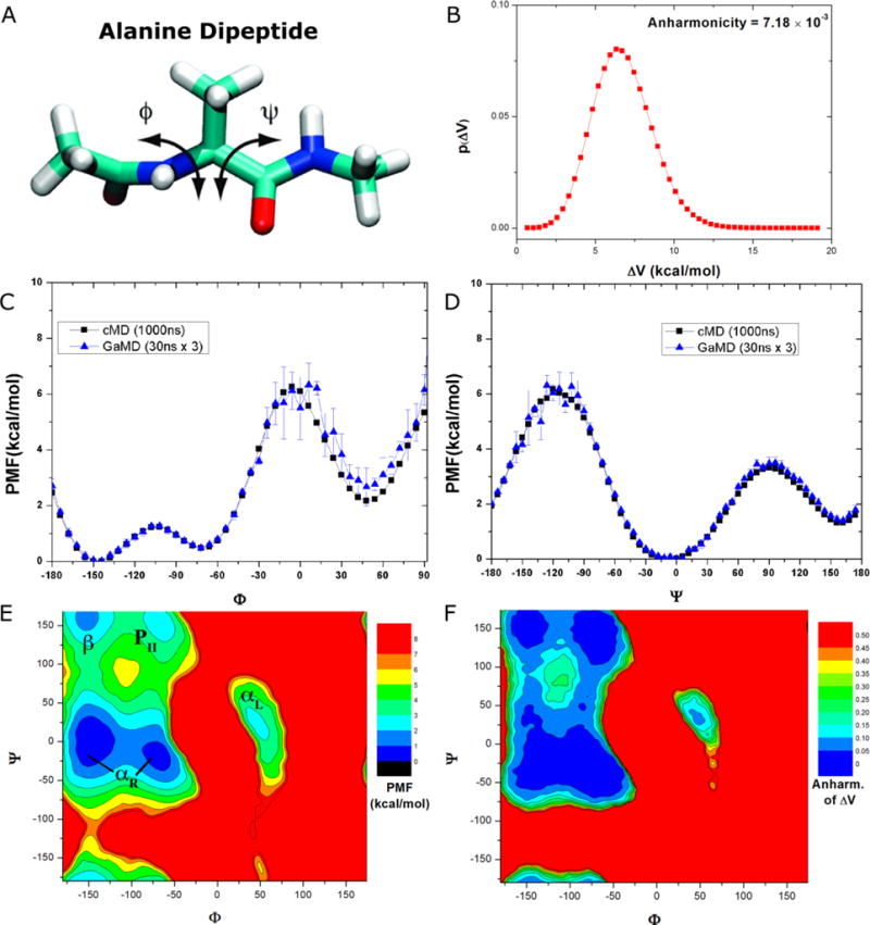
Demonstration of GaMD on the alanine dipeptide: (A) Schematic representation of backbone dihedrals Φ and Ψ in alanine dipeptide. (B) Distribution of the boost potential applied in the GaMD simulations with anharmonicity equal to 7.18×10⁻³. (C-D) potential of mean force (PMF) profiles of the (C) Φ and (D) Ψ dihedrals calculated from three 30 ns GaMD simulations combined using cumulant expansion to the 2nd order. (E) The 2D PMF profile of backbone dihedrals (Φ, Ψ). The low energy wells are labeled corresponding to the right-handed α helix (αR), left-handed α helix (αL), β-sheet (β) and polyproline II (PII) conformations. (F) The distribution anharmonicity of of frames found in each bin of the PMF profile.
In comparison, the reweighted PMF profiles obtained from 30ns GaMD trajectories agree quantitatively with the original profiles from much longer 1000 ns cMD simulation. Although the GaMD derived PMF profile of Φ exhibits moderate fluctuations near the energy barrier at 0° and slightly elevated free energy well centered at ~50° (Figure 2C), it essentially overlaps with the original profile in the other regions, similar for the entire PMF profile of Ψ (Figure 2D). In contrast, three cMD simulations did not properly sample the energy barriers of Φ at 0° and Ψ at 120°40. For Φ, the energy well centered at 60° obtained from the 30 ns cMD simulations was higher than that from 1000 ns cMD simulation. Therefore, whereas cMD simulations performed for 30ns are poorly converged for alanine dipeptide, GaMD simulations of the same length yielded significantly improved free energy profiles that agree quantitatively with those of the 1000 ns cMD simulation.
In addition, we calculated a 2D PMF of (Φ, Ψ) in alanine dipeptide by reweighting the three 30 ns GaMD trajectories combined. As shown in Figure 2E, five free energy wells were identified in the reweighted PMF profile of (Φ, Ψ), which are centered around (−144°, 0°) and (−72°, −18°) for the right-handed α helix (αR), (48°, −6°) for the left-handed α helix (αL), (−150°, 156°) for the β-sheet and (−72°, 162°) for the polyproline II (PII) conformation (Figure 2E). Their corresponding minimum free energies are estimated as 0 kcal/mol, 0.47 kcal/mol, 1.82 kcal/mol, 1.44 kcal/mol and 2.35 kcal/mol, respectively. In addition, the distribution anharmonicity of of frames clustered in each bin of the 2D PMF is smaller than 0.10 in all low-energy regions (Figure 2F), suggesting that reweighting using 2nd order cumulant expansion is a reasonable approximation. Indeed, the reweighted 2D PMF profile obtained from three 30ns GaMD trajectories (Figure 2E) is very similar to that obtained from 1000ns cMD, but not for the 30 ns cMD simulations40.
Therefore, short GaMD simulations of the alanine dipeptide performed for only 30ns were able to reproduce highly accurate free energy profiles of the backbone dihedrals that may need as long as 1000 ns cMD simulation to converge. The free energy errors were almost negligible except the elevated free energy well of Φ near 50° by ~0.5 kcal/mol and slight fluctuations in the energy barriers (particularly Φ at 0° and Ψ at −120°) (Figures 2C and 2D). In contrast, cMD simulations lasting 30 ns hardly sample these free energy barriers and exhibit poor convergence40. These results show that GaMD-NAMD greatly accelerates the conformational sampling and accurate free energy calculation of the alanine dipeptide biomolecular model system.
4.2 Protein Folding
Simulation Protocol
GaMD was applied to simulate the folding of chignolin, which is a fast-folding protein with 10 amino acid residues. Simulations of chignolin were performed using the AMBER ff99SB force field on GPUs49, 50, 51, 52. The simulation system was built using the Xleap module of the AMBER package. By solvating chignolin in a TIP3P54 water box that extends 8 to 10 Å from the solute surface, the system contained 2,211 water molecules and 6,773 atoms in total. Periodic boundary conditions were applied for the simulation system. Bonds containing hydrogen atoms were restrained with the SHAKE algorithm55 and a 2fs timestep was used. Weak coupling to an external temperature and pressure bath was used to control both temperature and pressure56. The electrostatic interactions were calculated using the PME (particle mesh Ewald summation)57 with a cutoff of 8.0 Å for long-range interactions.
The system was initially minimized for 2,000 steps using the conjugate gradient minimization algorithm and then the solvent was equilibrated for 50 ps in isothermal-isobaric (NPT) ensemble with the solute atoms fixed. Another minimization was performed with all atoms free and the system was slowly heated to 300 K over 500 ps. Final system equilibration was achieved by a 200 ps isothermal-isovolumetric (NVT) and 400 ps NPT run to assure that the water box of simulated system had reached the appropriate density.
In GaMD simulations of chignolin, the system threshold energy is set as . The maximum, minimum, average and standard deviation values of the system potential ( , , and ) were obtained from an initial 2 ns NVT simulation with no boost potential. The GaMD simulation proceeds with 50 ns equilibration after adding the boost potential and then three independent 300 ns production runs using the dual-boost. The GaMD implemented in both AMBER and NAMD has been applied to simulate chignolin yielding similar results39, 40, although certain difference was found in the calculated free energy profiles, which will be described below. We will present results mainly obtained from GaMD-NAMD40 in the following.
Simulation Results
Starting from an extended conformation of chignolin, GaMD simulations were able to capture complete folding of the protein into its native structure within 300 ns. The RMSD obtained between the simulation-folded chignolin and NMR experimental native structure (PDB: 1UAO) reaches a minimum of 0.2 Å (Figure 3A). The system boost potential applied in the GaMD simulations followed Gaussian distribution with the anharmonicity equal to 9.66×10⁻³ (Figure 3B). The average and standard deviation of the boost potential are 11.2 kcal/mol and 2.8 kcal/mol, respectively. During the three independent 300ns GaMD simulations, chignolin folded into the native conformational state with RMSD < 2 Å and unfolded repeatedly in two of the simulations. It remained in the folded state after rapid folding within ~20 ns in the third simulation (Figure 3C). Upon folding, the chignolin showed decrease of the radius of gyration, Rg, to 4.2 Å (Figure 3D).
Figure 3.
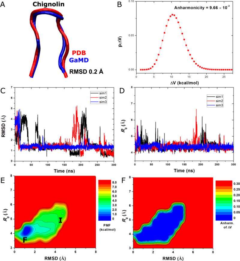
GaMD simulations of protein folding as demonstrated for chignolin: (A) comparison of simulation-folded chignolin (blue) with the PDB (1UAO) native structure (red) that exhibits 0.2 Å RMSD, (B) distribution of the boost potential , (C) 2D (RMSD, Rg) PMF calculated by reweighting the three 300 ns GaMD simulations combined and (D) the distribution anharmonicity of of frames found in each bin of the PMF profile.
Based on the Gaussian distribution of the boost potential, cumulant expansion to 2nd order was applied to reweight the combined three 300 ns GaMD simulations of chignolin. A 2D PMF profile was calculated for the protein RMSD relative to the PDB native structure and the radius of gyration, (RMSD, Rg) as shown in Figure 3E. The reweighted PMF allowed us to identify the folded (“F”) and intermediate (“I”) conformational states, which correspond to the global energy minimum at (1.0 Å, 4.0 Å) and a low-energy well centered at (4.5 Å, 5.5 Å), respectively. Figure 3F plots the distribution anharmonicity of for frames found in each bin of the 2D PMF as shown in Figure 3E. The anharmonicity exhibits values smaller than 0.05 in the simulation sampled conformational space, suggesting that the boost potential follows Gaussian distribution for proper reweighting using cumulant expansion to the 2nd order. Therefore, GaMD enables efficient enhanced sampling and free energy calculations of protein folding as demonstrated on the chignolin.
In summary, the GaMD-NAMD simulations were able to fold the protein rapidly. In two of the three 300ns GaMD simulations, chignolin undergoes both folding and unfolding repeatedly (Figure 3C). Compared with the average folding time obtained from long-timescale cMD simulations (600 ns)58, GaMD folds the protein within ~28 ns, i.e., ~30 times faster. Unlike the previous GaMD-AMBER simulations39, the fully unfolded state of chignolin does not appear as a low-energy well in the reweighted free energy profile obtained from the present GaMD-NAMD simulations. This behavior will be subject to further investigation in future GaMD studies. Nonetheless, in addition to sampling the folded state in the global free energy minimum, the GaMD-NAMD simulations also captured the intermediate state during the folding of the protein. This is consistent with the previous long-timescale cMD58 and aMD38 simulations.
4.3 Biomolecular Conformational Transitions: G-Protein-Coupled Receptors (GPCRs)
G-protein-coupled receptors (GPCRs) represent primary targets of about one third of currently marketed drugs. The structure, dynamics and function of GPCRs result from complex free energy landscapes6. Here, we have applied the GaMD method to study the ligand-dependent behavior of the M2 muscarinic GPCR. The M2 muscarinic receptor is widely distributed in mammalian tissues. It plays a key role in regulating the human heart rate and heart contraction forces. The M2 receptor has been crystallized in both an inactive state bound by the inverse agonist 3-quinuclidinyl-benzilate (QNB)59 and an active state bound by the full agonist iperoxo (IXO) and a G protein mimetic nanobody60. The receptor activation is characterized by rearrangements of the transmembrane (TM) helices 5, 6 and 7, particularly closing of the ligand-binding pocket, outward tilting of the TM6 cytoplasmic end and close interaction of Tyr2065.58 and Tyr4407.53 in the G protein-coupling site60. The residue superscripts denote the Ballesteros-Weinstein (BW) numbering of GPCRs61. Extensive GaMD simulations have revealed distinct structural flexibility and free energy profiles that depict graded activation of the M2 receptor. We have unprecedentedly captured both dissociation and binding of an orthosteric ligand in a single all-atom GPCR simulation, which will be described in Section 4.4.3.
Simulation Protocol
GaMD simulations were performed on the M2 muscarinic GPCR that is bound by the full agonist IXO, partial agonist arecoline (ARC)62 and inverse agonist QNB, in the presence or absence of the G protein mimetic nanobody Nb9-8. The CHARMM36 parameter set63 was used for the M2 receptor, G-protein mimetic nanobody and POPC lipids. Force field parameters of QNB were obtained from the CHARMM ParamChem web server and QNB was simulated in the protonated state as described previously64. For full agonist IXO and partial agonist ARC, the force field parameters were computed using the General Automated Atomic Model Parameterization (GAAMP) tool65. By using ab initio quantum mechanical calculations, GAAMP65 generates force field parameters that are compatible with CHARMM as used for protein and lipids36.
For each of the M2 receptor complex systems, initial energy minimization, thermalization and 100 ns cMD equilibration were performed using NAMD 2.1042. A cutoff distance of 12 Å was used for the van der Waals and short-range electrostatic interactions and the long-range electrostatic interactions were computed with the particle-mesh Ewald summation method using a grid point density of 1/Å. A 2 fs integration time-step was used for all MD simulations and a multiple-time-stepping algorithm was employed with bonded and short-range nonbonded interactions computed every time-step and long-range electrostatic interactions every two time-steps. The SHAKE algorithm was applied to all hydrogen-containing bonds. The NAMD simulation started with equilibration of the lipid tails. With all other atoms fixed, the lipid tails were energy minimized for 1000 steps using the conjugate gradient algorithm and melted with an NVT run for 0.5 ns at 310 K. The two systems were further equilibrated using an NPT run at 1 atm and 310 K for 10 ns with 5 kcal/(mol·Å2) harmonic position restraints applied to the crystallographically-identified atoms in the protein and ligand. The system volume was found to decrease with a flexible unit cell applied and level off within 10 ns NPT run, suggesting that solvent and lipid molecules in the system were well equilibrated. Final equilibration of each system was performed using an NPT run at 1 atm and 310 K for 0.5 ns with all atoms unrestrained. After energy minimization and system equilibration, a cMD simulation was performed on each system for 100 ns at 1 atm pressure and 310 K with a constant ratio constraint applied on the lipid bilayer in the X-Y plane.
With the NAMD output structure, together with the system topology and CHARMM36 force field files, the ParmEd tool in the AMBER package was used to convert the simulation files into the AMBER format41. The GaMD module implemented in the GPU version of AMBER1439, 41 was then applied to perform the GaMD simulation, which included a 10 ns short cMD simulation to collect the potential statistics for calculating GaMD acceleration parameters, a 50 ns equilibration after adding the boost potential, and finally multiple independent GaMD production simulations with randomized initial atomic velocities. All GaMD simulations were run at the “dual-boost” level by setting the reference energy to the lower bound, i.e., 39. One boost potential is applied to the dihedral energetic term and another to the total potential energetic term. The average and standard deviation of the system potential energies were calculated every 200,000 steps (400 ps) and 250,000 (500 ps) steps for the nanobody-free and nanobody-bound complex systems, respectively. The upper limit of the boost potential standard deviation, was set to 6.0 kcal/mol for both the dihedral and total potential energetic terms. Similar temperature and pressure parameters were used as in the NAMD simulations. GaMD production simulations were performed on the different M2 receptor complex systems at 400 - 2030 ns lengths. The simulation frames were saved every 0.1 ps for analysis.
Simulation Results
Detailed ligand-dependent dynamics and free energy profiles of the M2 muscarinic GPCR were obtained through the GaMD simulations (~19 μs in total). The receptor orthosteric pocket exhibits both closed and open conformations (Figure 4A), for which the “Tyrosine lid”60 composed of residues Tyr1043.33, Tyr4036.51 and Tyr4267.39 samples free energy minima at ~30 Å and ~33 Å, respectively (Figure 4C). In the presence of the G protein mimetic nanobody, IXO shifts the receptor conformational equilibrium to the closed state. In contrast, the orthosteric pocket interconverts dynamically between the closed and open states when the ligand is changed from IXO to ARC in the nanobody-coupled receptor, although the extracellular vestibule remains to adopt the narrowest opening48. Without the nanobody, QNB confines the receptor orthosteric pocket in the open state. ARC and IXO, however, yield a significantly broader energy well covering both the open and closed states although the open state is favored. Given such plasticity, the orthosteric pocket of the M2 receptor is able to accommodate different ligands of various sizes60, 62. In addition, the extracellular vestibule in the IXO- and ARC-bound receptor samples both the narrow and wide opening conformations, for which the distances between Tyr177ECL2−Asn4106.58 are 12.5 Å and ~16 Å, respectively48. Overall, the extracellular vestibule appears highly flexible. Binding of allosteric modulators may stabilize it in specific conformations and alter the orthosteric ligand-mediated responses60, 66.
Figure 4.
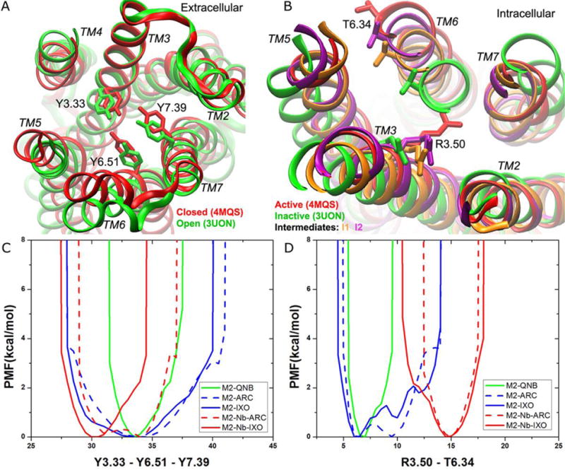
GaMD simulations revealed distinct low-energy states of the M2 muscarinic GPCR in the orthosteric ligand-binding and intracellular G protein coupling sites: (A) The orthosteric site exhibits closed (red, 4MQS X-ray) and open (green, 3UON X-ray) conformations. (B) The G protein coupling site samples inactive (green, 3UON X-ray), intermediates “I1” (orange), “I2” (purple) and active (red, 4MQS X-ray) conformational states. (C-D) The 1D PMF profiles of (C) the Tyr1043.33−Tyr4036.51−Tyr4267.39 triangle perimeter and (D) the Arg1213.50−Thr3866.34 distance calculated for the M2-QNB, M2-ARC, M2-IXO, M2-nanobody-ARC and M2-nanobody-IXO complex systems.
The G protein-coupling site samples the inactive, intermediates “I1” and “I2”, and active conformational states (Figure 4B), for which low-energy minima are found for the Arg1213.50−Thr3866.34 distance at 6.0-7.0 Å, ~10 Å, ~12 Å, ~15 Å, respectively (Figure 4D). QNB confines the receptor in the inactive state, while binding of IXO and ARC, together with the nanobody, shifts the receptor to the fully active state. In contrast, the full/partial agonist alone allows the receptor to sample more than one low-energy state. The M2-ARC complex samples the inactive and intermediate “I1” states with similar free energies. In addition, IXO shifts the conformational equilibrium further and allows the receptor to visit the intermediate “I2” state.
Overall, the M2 receptor samples a large conformational space (Figure 5). In the presence of the G protein mimetic nanobody, the receptor is stabilized in the fully active state with the most open intracellular pocket and the narrowest extracellular vestibule. In the orthosteric pocket, IXO stabilizes the receptor in the closed state, while ARC binding allows the receptor to change between the closed and open states with two alternative conformations (ARC-P1 and ARC-P1′)48. Such dynamic binding of the partial agonist, along with multiple associated receptor conformations, has previously been observed in NMR experiments of the peroxisome proliferator-activated receptor γ67.
Figure 5.
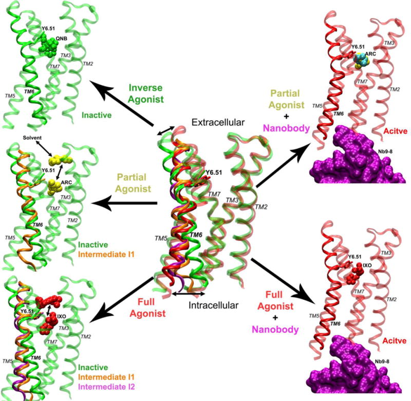
Mechanism of graded activation of the M2 muscarinic GPCR: The M2 receptor (ribbons) samples a large conformational space with significant structural rearrangements, especially for the TM6 helix. Binding of the inverse agonist QNB (green spheres) confines the receptor in the inactive state. Without the G protein or mimetic nanobody, the partial agonist ARC (yellow spheres) biases the M2 receptor to visit an intermediate state “I1” (orange ribbons). ARC is able to dissociate completely to the bulk solvent via the extracellular vestibule and rebinds to the receptor repeatedly during a 2030 ns GaMD simulation. In comparison, the full agonist IXO (red spheres) biases the receptor further, sampling both intermediate “I1” (orange ribbons) and “I2” (purple ribbons). IXO escapes out of the orthosteric pocket and visits the extracellular vestibule in one of the GaMD simulations. By adding the G protein mimetic nanobody (purple surface), the M2 receptor is stabilized in the fully active state (red ribbons) as bound by IXO or ARC, although ARC adopts two alternative conformations in the orthosteric pocket, ARC-P1 (yellow spheres) and ARC-P1′ (cyan spheres).
Removal of the nanobody leads to deactivation of the M2 receptor with inward displacement of the TM6 cytoplasmic end. This is consistent with extensive experimental and computational studies of GPCRs, especially on the β2-adrenergic receptor (β2AR)68. Binding of QNB confines the receptor in the inactive state with the shortest distance between Arg1213.50−Thr3866.34 (~6-7 Å). Without the G protein or mimetic nanobody, ARC biases the receptor to visit an intermediate state “I1” that exhibits increased distance between Arg1213.50−Thr3866.34 (~10 Å). In comparison, IXO is able to bias the receptor further, sampling both intermediates “I1” and “I2” with ~10 Å and ~12 Å distances between Arg1213.50−Thr3866.34, respectively. Note that our earlier accelerated MD (aMD) simulations captured similar conformational change during activation of the apo M2 receptor that exhibits basal activity32. Even without agonist binding, the apo receptor undergoes transient outward movement of the TM6 cytoplasmic end up to ~12 Å. To a certain extent, the intermediate “I2” in the present study can be considered as an “active-like” state, which has been used to define the agonist-bound adenosine A2A receptor (A2AAR)69. In summary, graded activation of the M2 receptor is characterized by outward movement of the TM6 cytoplasmic end at increasing magnitudes when the ligand changes from inverse to partial and full agonists.
4.4 Biomolecular Recognition
4.4.1 Ligand binding of the T4-lysozyme
Simulation Protocol
GaMD simulations of ligand binding to the T4-lysozyme were performed using the AMBER ff99SB force field on GPUs49, 50, 51, 52. The simulated systems were built using the Xleap module of the AMBER package. The ligand benzene was removed from the X-ray crystal structure of the Leu99Ala mutant (PDB: 181L)70. Another four benzene molecules were placed in the bulk solvent at least 40 Å away from the ligand-binding site in the starting configuration. By solvating T4-lysozyme in a TIP3P54 water box that extends 8 to 10 Å from the solute surface, the system contained 9,011 water molecules and 29,692 atoms in total. Five independent 800 ns dual-boost GaMD simulations were initially performed. Complete binding of benzene to the target ligand-binding site was observed in one of the five simulations. Even when the simulation was extended to 1,800 ns, benzene remained tightly bound in the ligand-binding cavity. The simulation frames were saved every 0.1 ps for analysis.
Simulation Results
GaMD captured complete binding of benzene to the deeply buried ligand-binding cavity in the T4-lysozyme within ~100 ns in one of the five independent 800 ns simulations. Benzene remained bound in ligand-binding site even when the simulation was extended to 1,800 ns. As shown in Figure 6A, Benzene diffuses from the bulk solvent to the protein surface formed by the αD and αG helices and then to the target ligand-binding site in the protein C-terminal domain. In the intermediate state, benzene interacts with residues Lys83, Pro86 and Val87 from the αD helix and the Thr115, Thr119 and Gln122 residues from the αG helix (Figure 6B). In the bound pose (the binding position and orientation of a ligand at a protein target site), benzene is superimposable with the ligand co-crystallized in the 181L crystal structure. By aligning the C-terminal domain (residues 80-160) of the T4-lysozyme, the RMSD of the diffusing benzene molecules relative to the bound pose in the 181L X-ray crystal structure reaches a minimum of 0.1 Å (Figure 6C). It forms hydrophobic interactions with residues Ile78, Leu84, Tyr88, Val87, Leu91, Val111, Leu118 and Leu121 in the deeply buried protein cavity39.
Figure 6.
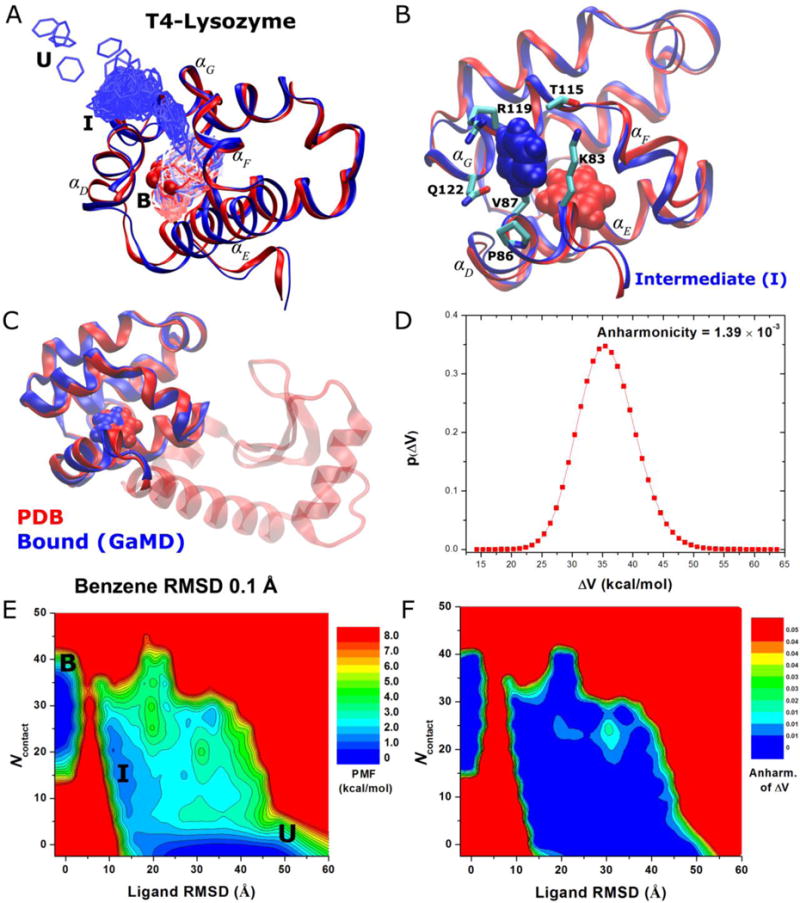
GaMD simulations captured binding of ligand benzene to the T4-lysozyme: (A) A pathway of benzene binding to the T4-lysozyme observed during the GaMD simulation. (B) The intermediate (“I”) poses of the protein-ligand complex (blue) with the protein C-terminal domain (residues 80-160) aligned to the PDB native structure (red). The protein and benzene are represented by ribbons and spheres, respectively, and they are colored by blue for the simulation structure with red for the PDB native structure, except that in (A) the simulated benzene is represented by lines and colored by simulation time in a BWR color scale. Residues with heavy atoms found within 3 Å of benzene are represented by sticks. (C) Comparison of simulation-derived complex structure that captures benzene binding (blue) with 0.1 Å ligand RMSD relative to the 181L PDB structure (red), (D) distribution of the boost potential , (E) 2D (Ligand RMSD, Ncontact) PMF calculated by reweighting the 1,800 ns GaMD simulation and (F) the distribution anharmonicity of of frames found in each bin of the free energy profile.
The boost potential applied during the 1,800 ns GaMD simulation follows Gaussian distribution and its distribution anharmonicity γ equals 1.39×10⁻³ (Figure 6D). The average and standard deviation of are 36.5 kcal/mol and 4.7 kcal/mol, respectively. Although the average values exhibit variations between five independent simulations, the standard deviations are closely similar to each other provided that ( , ) were set to (3.0, 4.0).
Using the RMSD of benzene relative to the bound pose and the number protein heavy atoms that are within 5 Å of benzene (Ncontact) with a bin size of (1.0 Å, 5), a 2D PMF profile was calculated by reweighting the 1,800 ns GaMD simulation (Figure 6E). The reweighted PMF allows us to identify three distinct low-energy states: the unbound (“U”), intermediate (“I”) and bound (“B”) states. The bound state corresponds to the global energy minimum located at ~(0 Å, 30), the unbound state in a local energy well centered at ~(33 Å, 0) and the intermediate centered at ~(11 Å, 20). It is important to note that since the complete binding of benzene to the target ligand-binding site was observed only once, the calculated binding free energy between the bound and unbound states is subject to the error of limited sampling. Nevertheless, benzene visits the intermediate site many times during the 1800 ns GaMD simulation with the ligand RMSD decreased to ~11 Å (Figure 6E)39. Repeated sampling of the intermediate state was observed in the other four 800 ns GaMD simulations as well, for which a local energy well appears around (11.0 Å, 20) in the 2D PMF profiles39. The relative free energy between the intermediate and unbound states is estimated to be 0.53±0.46 kcal/mol from PMF profiles of the five GaMD simulations. Furthermore, benzene was observed to bind another intermediate 2 (“I2”) site that is located in the pocket formed by the hinge αC helix and the αB helix from the N-terminal domain39. A corresponding local energy well of the I2 state appears in the calculated 2D PMF profiles. Figure 6F plots the distribution anharmonicity, γ for frames found in each bin of the 2D PMF. It exhibits relatively large values in the high-energy regions (less sampling), notably the energy barrier between the intermediate and bound states. The ligand entry from the intermediate to the bound state is thus suggested to be the rate-limiting step for benzene binding. In comparison, γ exhibits values smaller than 0.01 in the energy well regions, suggesting that achieves sufficient sampling for reweighting using cumulant expansion to the 2nd order.
In summary, GaMD captured complete binding of benzene to the ligand-binding site of the T4-lysozyme. Distinct low-energy unbound, intermediate and bound states were identified from the reweighted free energy profiles. The atomistic GaMD simulation also elucidates a highly detailed binding pathway of benzene that diffuses from the bulk solvent to an intermediate site located on the protein surface formed by the αD and αG helices, and then slides into the target ligand-binding cavity through a channel formed by the αD, αF and αG helices. The free energy difference between the intermediate and unbound states was found to be small at 0.53 ± 0.46 kcal/mol as estimated from the five independent GaMD simulations. Benzene repeatedly visits the intermediate site on the protein surface. In comparison, the ligand entry from protein surface to the deeply buried protein cavity appears to be the rate-limiting step for complete benzene binding. It is important to note that the complete ligand binding was not observed in the four 800 ns GaMD simulations, suggesting that the present GaMD simulations still suffer from insufficient sampling of the ligand entry process and the reweighted free energy profiles remain un-converged. This is also indicated by the increased anharmonicity corresponding to the free energy barrier between the intermediate and bound states as shown in Figure 6F. Nevertheless, our GaMD simulation captured a binding pathway of benzene to the T4-lysozyme. The ligand entry site is indeed adjacent to the mobile αF helix (residues 108-113), which has been suggested earlier71, 72, 73 based on the finding that the αF helix exhibit increased B-factors in the Leu99Ala complex structures compared to the apo structures70, 74, 75.
4.4.2 Ligand Binding of the M3 Muscarinic GPCR
The GaMD implemented in NAMD 2.1140 was applied to simulate binding of the endogenous agonist acetylcholine (ACh) to the M3 muscarinic GPCR (Figure 7). The M3 muscarinic receptor is widely expressed in human tissues and a key seven-transmembrane (TM) GPCR that has been targeted for treating various human diseases, including cancer76, diabetes77, 78 and obesity79.
Figure 7.
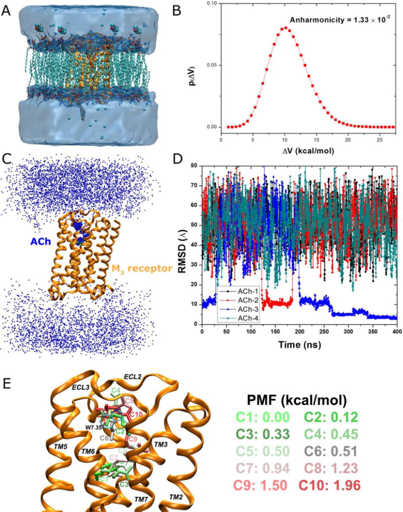
GaMD simulations captured binding of the acetylcholine (ACh) endogenous agonist to the M3 muscarinic GPCR: (A) schematic representation of the computational model, in which the receptor is shown in ribbons (orange), lipid in sticks, ions in small spheres and four ligand molecules in large spheres, (B) distribution of the boost potential with anharmonicity equal to 1.33×10⁻², (C) probability distribution of the ACh (the N atom in blue dots) diffusing in the bulk solvent and bound to the M3 receptor (orange ribbons), in which the Glide docking pose of ACh is shown in green sticks, (D) the RMSD of the diffusing ACh relative to the Glide docking pose calculated from the 400 ns GaMD simulation, and (E) Ten lowest energy structural clusters of ACh that are labeled and colored in a green-white-red (GWR) scale according to the PMF values obtained from reweighting of the GaMD simulation.
Simulation Protocol
Simulations of the M3 muscarinic receptor were carried out using the inactive tiotropium (TTP)-bound X-ray structure (PDB: 4DAJ) that was determined at 3.40 Å resolution59. To simulate the ligand binding, TTP was removed from the X-ray structure. The T4 lysozyme that was fused into the protein to replace intracellular loop 3 (ICL3) for crystallizing the receptor was omitted from all simulations, based on previous findings that removal of the bulk of ICL3 does not appear to affect GPCR function and ICL3 is highly flexible68. All chain termini were capped with neutral groups (acetyl and methylamide). Two disulphide bonds that were resolved in the crystal structure, i.e., C1403.25-C220ECL2 and C5166.61-C5197.29, were maintained in the simulations. Using the psfgen plugin in VMD80, the Asp1132.50 residue was protonated as in previous microsecond-timescale Anton simulations64. All other protein residues were set to the standard CHARMM protonation states at neutral pH64, including the deprotonated Asp1473.32 residue in the orthosteric site33, 36.
The M3 receptor was inserted into a palmitoyl-oleoyl-phosphatidyl-choline (POPC) bilayer with all overlapping lipid molecules removed using the Membrane plugin and solvated in a water box using the Solvate plugin in VMD80. Four ligand molecules were placed at least 40 Å away from the receptor orthosteric site in the bulk solvent of the starting structures (Figure 7A). The system charges were then neutralized with 18 Cl− ions. The simulation systems of the M3 receptor initially measured about 80 × 87 × 97 Å3 with 130 lipid molecules, ~11,200 water molecules and a total of ~55,500 atoms. Periodic boundary conditions were applied to the system.
Initial energy minimization and thermalization of the M3 receptor system follow the same protocol as used in a previous study36. GaMD simulation was then performed using the dual-boost scheme with the threshold energy E set to Vmax. The GaMD simulations included 2 ns cMD, 50 ns equilibration after adding the boost potential and then three independent production runs with randomized atomic velocities (one for 400 ns and another two for 300 ns). The GaMD simulations were carried out using NAMD 2.11 on the Gordon supercomputer at the San Diego Supercomputing Center. Benchmark simulations showed that GaMD ran at ~10 ns/day with 64 CPUs and up to ~61 ns/day with 640 CPUs, which were ~8 to 11% slower than the corresponding cMD runs. This performance is very similar to that of the conventional aMD implemented in NAMD47. GaMD production frames were saved every 0.1 ps. The VMD80 and CPPTRAJ81 tools were used for trajectory analysis. The Density Based Spatial Clustering of Applications with Noise (DBSCAN) algorithm82 was applied to cluster the diffusing ligand molecules for identifying the highly populated binding sites. Finally, the PyReweighting toolkit37 was applied to compute the potential of mean force (PMF) profiles of structural clusters of the diffusing ACh.
Simulation Results
Analysis of GaMD simulations on the M3 muscarinic GPCR showed that the system boost potential follows Gaussian distribution with anharmonicity equal to 1.33×10⁻² (Figure 7B). The average and standard deviation of the boost potential are 10.9 kcal/mol and 3.0 kcal/mol, respectively. Such narrow distribution will ensure accurate reweighting for free energy calculation using cumulant expansion to the 2nd order.
During the 400 ns GaMD simulation of the M3 muscarinic receptor, ACh was observed to enter the receptor and then bind to the receptor endogenous ligand-binding (“orthosteric”) site (Figure 7C). Highly populated clusters were identified for the ligand in the extracellular vestibule and orthosteric site of the receptor, while the ligand diffuses nearly homogenously in the bulk solvent. Note that periodic boundary conditions were applied on the simulation system and thus ACh diffused to the cytoplasmic side of the lipid membrane, which may not occur in the real cells. Nonetheless, ACh entered the receptor from only the extracellular side, recapitulating the first step of GPCR-mediated cellular signaling machinery. Figure 7D plots the RMSD of the four diffusing ACh molecules relative to the ligand binding pose predicted from Glide docking83, 84 in the orthosteric site. The ACh-3 molecule was observed to bind the extracellular vestibule with ~10 Å RMSD, dissociate completely from the receptor, rebind to the extracellular vestibule at ~200ns and then enter the receptor to the orthosteric pocket at ~270 ns. It finally rearranged its conformation in the orthosteric pocket, reached a minimum RMSD of 2.0 Å at ~340 ns and stayed bound in the orthosteric site until the end of the 400 ns GaMD simulation. Moreover, during the dissociation of the ACh-3, another ligand molecule (ACh-2) bound briefly to the receptor extracellular vestibule during ~125-180 ns. Similar observations were obtained in the other 300 ns GaMD simulations of the M3 receptor40, during which different ACh molecules were able to bind the extracellular vestibule but could not reach the orthosteric site within the limited simulation time.
In order to obtain a quantitative picture of the ligand binding pathway, the DBSCAN algorithm82 was applied to cluster trajectory snapshots of four diffusing ligand molecules from the 400 ns GaMD simulation. Energetic reweighting37, 39 was then applied to each of the ligand structural clusters to recover the original free energy. Ten structural clusters with the lowest free energies are shown in Figure 7E. Global free energy minimum (0.0 kcal/mol) was found for cluster “C1” in the orthosteric site. The second lowest energy minimum was identified for cluster “C2” (0.12 kcal/mol) located in the extracellular vestibule formed between ECL2/ECL3. Moreover, cluster “C3”, which exhibits a different conformation compared with cluster “C1” and higher free energy (0.33 kcal/mol), was also identified in the orthosteric pocket. In addition to cluster “C2”, clusters “C4” with 0.45 kcal/mol, “C6” with 0.51 kcal/mol, “C8” with 1.23 kcal/mol and “C10” with 1.96 kcal/mol were also identified in the extracellular vestibule, in which the positively charged N atom of the ligand interacts with residue Trp5257.35 through cation-π interactions. The residue superscripts denote the Ballesteros-Weinstein (BW) numbering of GPCRs61. Three clusters of higher free energies, “C5” with 0.50 kcal/mol, “C7” with 0.94 kcal/mol, “C9” with 1.50 kcal/mol, appear to connect “C1” in the orthosteric pocket and “C2” in the extracellular vestibule. Therefore, structural clusters “C1”, “C3” ↔ “C7”, “C5”, “C9” ↔ “C2”, “C4”, “C6”, “C8”, “C10” appear to represent an energetically preferred pathway for the endogenous agonist binding to the M3 muscarinic receptor.
In summary, GaMD-NAMD was demonstrated to be of use for ligand binding to the M3 muscarinic GPCR as a model membrane protein system. While the ACh endogenous agonist binds only transiently to the receptor extracellular vestibule in two 300 ns GaMD simulations, the ligand enters the receptor and binds to the target orthosteric site in a 400 ns GaMD simulation. Although, in principle, multiple binding and unbinding events may be needed in order to compute converged ligand binding free energy, structural clustering and reweighting of the GaMD simulation allows us to identify energetically preferred binding sites and pathway of the diffusing ligand. Particularly, the lowest energy cluster of ACh is identified in the orthosteric site, in excellent agreement with the Glide docking pose. The second lowest energy cluster is located in the extracellular vestibule, with the positively charged N atom of ACh forming cation-π interaction with the receptor residue Trp5257.35. This is consistent with previous extensive experimental and computational studies which showed that the extracellular vestibule of class A GPCRs acts as a metastable intermediate site during binding of orthosteric ligands36, 64. The energetically preferred pathway of agonist binding to the M3 receptor identified from the current GaMD-NAMD simulation is similar to that found in previous long-timescale cMD85 and aMD36 of class A GPCRs.
4.4.3. Ligand Dissociation and Binding of the M2 Muscarinic GPCR
Simulation Protocol
GaMD simulations of the M2 muscarinic GPCR, which is bound by the full agonist IXO, partial agonist arecoline (ARC) and inverse agonist QNB, are the same as described in Section 4.3. For each of the receptor complexes, initial energy minimization, thermalization and 100 ns cMD equilibration were performed using NAMD2.1042. Using the NAMD output structure, together with the system topology and CHARMM3663 force field files, ParmEd was used to convert the simulation files into the AMBER format41. The GaMD module implemented in the GPU version of AMBER1439, 41 was then applied to perform GaMD simulation, which included 10 ns short cMD simulation used to collect potential statistics for calculating the GaMD acceleration parameters, 50 ns equilibration after adding the boost potential and finally multiple independent GaMD production runs with randomized initial atomic velocities. The simulation frames were saved every 0.1 ps for analysis.
The DBSCAN algorithm82 implemented in CPPTRAJ was applied to cluster trajectory frames of the diffusing ARC and IXO by combining all the GaMD production simulations of the M2-ARC and M2-IXO systems, respectively. A total length of ~9100 ns GaMD simulation (~91 million frames) was obtained for ARC clustering. Because of the large data set, the frames were sieved at a stride of 2000 for clustering. A distance cutoff of 1.6 Å and minimum number of 80 sieved frames were set for forming a cluster. The remaining frames were assigned to the closest cluster afterwards. Similar parameters were used to cluster the M2-IXO simulation (total ~6300 ns), except that a minimum number of 10 sieved frames were set for forming a cluster. The PyReweighting37 toolkit was used to reweight ligand structural clusters to compute the free energy values.
Simulation Results
Whereas the inverse agonist QNB with high binding affinity (~0.06 nM)60 remains tightly bound to the orthosteric site, the full and partial agonists with lower affinities, ~5 μM for ARC62, 86 and ~0.01 μM for IXO60, exhibit significantly higher fluctuations. During one of the GaMD simulations, IXO escapes out of the orthosteric pocket and visits the extracellular vestibule48. For ARC, not only does it escape out of the orthosteric pocket, but it also dissociates completely and rebinds to the receptor repeatedly during a 2030 ns GaMD simulation. This was indicated by the timecourse of the ligand-Asp1033.32 distance (Figure 8A). Four dissociation (denoted “D1”, “D2”, “D3” and “D4”) and three binding (denoted “B1”, “B2” and “B3”) events took place. ARC exited the receptor via three extracellular openings, one formed between ECL2/ECL3 (“D1”, Figure 8B), the second between ECL2/TM2/TM7 (“D2”, Figure 8F) and another between ECL2/TM7 (“D3” and “D4”, Figures 8G and 8H). ARC rebound to the receptor through two of the three openings, i.e., ECL2/ECL3 (“B1”, Figure 8C) and ECL2/TM7 (“B2” and “B3”, Figures 8D and 8E).
Figure 8.
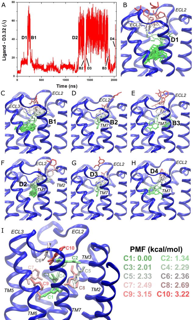
GaMD simulations revealed pathways of dissociation and binding of the arecoline (ARC) partial agonist of the M2 muscarinic GPCR: (A) Timecourse of the ARC−Asp1033.32 distance during 2030 ns GaMD simulation. Four dissociation and three binding events are labeled. (B-H) Schematic representations of the ligand pathways during (B) “D1”, (C) “B1”, (D) “B2”, (E) “B3”, (F) “D2”, (G) “D3” and (H) “D4”. The receptor is represented by blue ribbons and the ligand by sticks colored by the position along the membrane normal. (I) Ten lowest energy structural clusters of ARC that are labeled and colored in a GWR scale according to the PMF values.
With DBSCAN structural clustering and energetic reweighting, ten ligand clusters with the lowest free energies are shown in Figure 8I. Global energy minimum (0 kcal/mol) is found for cluster “C1” in the orthosteric pocket. The second lowest energy is identified for cluster “C2” (1.34 kcal/mol) at the center of the extracellular vestibule between ECL2/TM7. Two clusters of higher energies, “C3” with 2.01 kcal/mol and “C4” with 2.29 kcal/mol, appear to connect “C1” in the orthosteric pocket and “C2” in the extracellular vestibule. A cavity formed by the extracellular domains of TM3/TM2/TM7 is filled with two clusters, “C5” (2.33 kcal/mol) and “C8” (2.69 kcal/mol). Similarly, another cavity formed by the TM4/TM5/TM6 extracellular domains is filled with clusters “C7” and “C9” with 2.49 kcal/mol and 3.15 kcal/mol free energies, respectively. In the extracellular vestibule, although ARC was observed to exit between ECL2/TM2/TM7 in one of the dissociation events, this location does not appear among the ten lowest energy clusters. In contrast, two energetically favored clusters are found in the opening between ECL2/ECL3, i.e., “C6” (2.36 kcal/mol) and “C10” (3.22 kcal/mol). Therefore, clusters “C1”↔“C3”↔“C4”↔“C2”↔“C10”↔“C6” appear to represent an energetically preferred pathway for ARC dissociation and binding. IXO also follows a similar pathway during dissociation from the orthosteric site to the ECL2/ECL3 opening and rebinding to the center of the extracellular vestibule48.
Therefore, a pathway connecting the orthosteric site, center of the extracellular vestibule and the ECL2/ECL3 opening appears to be energetically favorable for ligand dissociation and binding of the M2 muscarinic receptor (Figure 8I). This route has also been identified as the dominant pathway for drug binding to β2AR85. Therefore, it is likely a common pathway adopted by class A GPCRs for ligand recognition, although this may also depend on the structural arrangement of the receptor extracellular domains and ligand size and chemical properties. For the M2 receptor, it is worth investigating the binding of more ligands and associated receptor dynamics in the future, e.g., the N-methylscopolamine and atropine inverse agonists62, the pilocarpine and McN-A343 partial agonists that elicit more consistent partial response of the M2 receptor62, 86, etc. In this context, although ligand dissociation from β2AR was simulated in a previous random acceleration MD (RAMD) study87, it was difficult to capture rebinding of the ligand. The ligand was observed to exit with similar probability via the ECL2/ECL3 and ECL2/TM2/TM7 openings, but the RAMD simulations could not differentiate the two pathways energetically. Another steered MD study on ligand dissociation from the β-ARs88 also suggested that the two routes “may serve indistinguishably for ligand entry and exit”. Although free energy profiles were obtained from the steered MD simulations, the ligand was constrained to predetermined CAVER channels, which may not reflect the real pathways as observed in the cMD simulations85. In comparison, GaMD provides unconstrained enhanced sampling and allows for free ligand diffusion. The simulation-derived free energy profiles can be used to characterize the ligand pathways quantitatively. Notably, the orthosteric pocket and extracellular vestibule were calculated as two low-energy binding sites of ARC. This is consistent with previous binding assay experiments, suggesting that several partial agonists have two or more binding sites in the M2 receptor62, 89. Earlier computational studies also identified the extracellular vestibule as a metastable site during binding of orthosteric ligands to the M2 and M3 muscarinic receptors36, 64. Therefore, GaMD is well suited for investigating ligand binding and dissociation of GPCRs and other large biomolecules.
5 Concluding Remarks
GaMD provides both unconstrained enhanced sampling and efficient free energy calculations of biomolecules. Important statistical properties of the system potential, such as the average, maximum, minimum and standard deviation values, are used to calculate the simulation acceleration parameters, particularly the threshold energy E and force constant k0. A minimal set of simulation parameters is dynamically adjusted to control the magnitude and distribution width of the boost potential. On one hand, GaMD does not require predefined reaction coordinates like many other enhanced sampling methods and thus enables unconstrained enhanced sampling90. On the other hand, within the new GaMD theoretical framework, the boost potential does not greatly change the shape of the overall biomolecular energy landscape. We are running near-equilibrium simulations in GaMD. As such, the resulting boost potential follows a Gaussian distribution and allows for accurate reweighting of the simulations using cumulant expansion to the second order.
In comparison with many enhanced sampling methods such as umbrella sampling13, 14, conformational flooding15, 16, metadynamics17, 18, ABF calculations19, 20 and orthogonal space sampling21, 22, GaMD has the advantage of no need to set predefined reaction coordinates. Metadynamics, in particular, is another potential biasing technique that has been widely used to map the free energy landscapes of biomolecules such as protein conformational changes91, 92 and protein-ligand binding18, 93. By monitoring the energy surface of biomolecules during the simulation, metadynamics keeps adding small Gaussians of potential energies to the low energy regions. This will eventually fill the low energy wells and achieve uniform sampling of the free energy surface along selected reaction coordinates. The usage of predefined coordinates greatly reduces the complexity of biomolecular simulation problems and facilitates the free energy calculations (e.g., significantly lower energetic noise compared with aMD simulations). However, it is key to select proper reaction coordinates, which often requires expert knowledge of the studied systems. Construction of biomolecular reaction coordinates or collective variables has thus been one of the main objectives in metadynamics studies17. When important reaction coordinates are missed during the simulation setup, metadynamics simulations may still suffer from slow convergence problems. In comparison, aMD simulations are not constrained by reaction coordinates, but this also leads to much higher energetic noise and presents grand challenge for accurate reweighting to recover the original free energy landscapes of biomolecules34. Although cumulant expansion to the 2nd order was shown to improve aMD reweighting when the boost potential follows near Gaussian distribution37, such improved reweighting is still limited to small systems such as protein with ≤ 35 residues38. Here, by constructing boost potential using a harmonic function that follows Gaussian distribution, GaMD enables rigorous energetic reweighting through cumulant expansion to the 2nd order, even for simulations of larger proteins (e.g., T4-lysozyme and GPCRs). With this, GaMD achieves simultaneous unconstrained enhanced sampling and free energy calculations.
GaMD has been implemented in AMBER39 and NAMD40, and this approach should be transferrable to other popular MD software packages, including GENESIS94, OpenMM95, etc. Notably, NAMD shows excellent scalability for supercomputer simulations of large biomolecules42. It is complementary to the implementation of GaMD in the graphics processing unit (GPU) version of AMBER39 that runs extremely fast simulations with one or a small number of GPU cards41, 51. As demonstrated on the model systems, these implementations facilitate the applications of GaMD in enhanced sampling and free energy calculations of a wide range of biomolecular systems, such as proteins, lipid membrane, nucleic acids, virus particles and cellular complex structures. Ongoing applications of GaMD also include the clustered regularly interspaced short palindromic repeats-CRISPR associated protein 9 (CRISPR-Cas9) system96, HIV protease, protein kinases, the acyl carrier proteins, and so on.
However, several cautions have also resulted from GaMD studies. First, while the present GaMD simulations seem to provide sufficient sampling of the low energy regions, they appear to remain unconverged in sampling of the high-energy barriers. This is particularly true for the ligand entry step in the GaMD simulation of benzene binding to the T4-lysozyme. It is worthy to recall that the threshold energy for adding the boost potential is set to its lower bound in the previous GaMD simulations. A subject of future investigation is whether using the upper bound of the threshold energy will facilitate sampling of the high-energy barriers in GaMD simulations.
Second, based on a potential biasing approach, GaMD mainly accelerates transitions across enthalpic energy barriers. Improvement for its application to systems with high entropic barriers is still needed. In this regard, GaMD can be potentially combined with the parallel tempering (PT)97 and replica exchange (RE)98, 99 algorithms like in replica-exchange aMD (REXAMD)99, 100 for further enhanced sampling. Particularly, the combination of parallel tempering and metadynamics (PT-MetaD)91 has been shown to facilitate enhanced sampling of biomolecules over entropic barriers. Moreover, the REXAMD that combines RE and aMD methods have been found helpful in free energy calculations101. Thus, one can combine GaMD that provides improved reweighting and RE for more accurate free energy calculations. In addition, we can use the essential potential energy as described in the essential energy space random walk (EESRW)102, 103, 104 method to improve the potential-biasing sampling methods such as GaMD.
Third, in order to obtain accurate free energy calculations, rigorous error analysis (particularly the reweighting) is still needed for GaMD. In this context, because the boost potential ΔV is physically equivalent to nonequilibrium work W, reweighting of aMD/GaMD simulations for calculating free energies can be expressed by the Jarzynski equality105: . When the three estimators and different aMD reweighting techniques examined in Refs.106 and 37 are compared, the mean work estimator is found equivalent to the approximation using Maclaurin series expansion, the fluctuation-dissipation (FD) theorem estimator corresponds to the cumulant expansion to the 2nd order (also referred to as the “Gaussian approximation”107) and the Jarzynski estimator corresponds to direct “exponential average” calculation. Detailed analysis showed that in the near-equilibrium regime, the mean work estimator gives comparatively larger errors and the Jarzynski estimator is more accurate than the FD estimator when the number of W (or ΔV) data points N≤16. However, the FD estimator gives the smallest error with increasing N (see Figure 4 in Ref. 106). This is consistent with our previous aMD reweighting study that shows the cumulant expansion to the 2nd order is the most accurate compared with the Maclaurin series expansion and exponential average, for which the number of ΔV values N used for aMD reweighting is on the order of 102−106 37. The bias and error of free energy calculations were examined rigorously in Ref. 106. Similar error estimates need to be performed for GaMD simulations when they are applied for free energy calculations.
In summary, without the need to set predefined reaction coordinates, GaMD is generally applicable to a wide range of biomolecular systems, including protein folding, biomolecular large-scale conformational transitions and biomolecular recognition as described in this chapter. For systems of increasing size, the upper limit of the standard deviation, can be adjusted dynamically to ensure that the distribution width of the applied boost potential is narrow enough for accurate energetic reweighting using cumulant expansion to the second order. Therefore, GaMD serves as a promising tool for biomolecular conformation sampling, prediction of drug-receptor interactions and computer-aided drug design and discovery108, 109.
Acknowledgments
This work was supported by NSF (grant MCB1020765), NIH (grants GM31749 and 1U01GM111528), American Heart Association (Award # 17SDG33370094), Howard Hughes Medical Institute, National Biomedical Computation Resource (NBCR), San Diego Supercomputer Center through the Extreme Science and Engineering Discovery Environment (Awards TG-MCA93S013 and TG-MCB140011), and the National Energy Research Scientific Computing Center (Project M1395).
References
- 1.Henzler-Wildman K, Kern D. Dynamic personalities of proteins. Nature. 2007;450(7172):964–972. doi: 10.1038/nature06522. [DOI] [PubMed] [Google Scholar]
- 2.Hatoum-Aslan A, Marraffini LA. Impact of CRISPR immunity on the emergence and virulence of bacterial pathogens. Curr Opin Microbiol. 2014;17:82–90. doi: 10.1016/j.mib.2013.12.001. [DOI] [PMC free article] [PubMed] [Google Scholar]
- 3.Englander SW, Mayne L. The nature of protein folding pathways. Proc Natl Acad Sci U S A. 2014;111(45):15873–15880. doi: 10.1073/pnas.1411798111. [DOI] [PMC free article] [PubMed] [Google Scholar]
- 4.Ritter SL, Hall RA. Fine-tuning of GPCR activity by receptor-interacting proteins. Nat Rev Mol Cell Biol. 2009;10(12):819–830. doi: 10.1038/nrm2803. [DOI] [PMC free article] [PubMed] [Google Scholar]
- 5.Onuchic JN, Luthey-Schulten Z, Wolynes PG. Theory of Protein Folding: The Energy Landscape Perspective. Annu Rev Phys Chem. 1997;48(1):545–600. doi: 10.1146/annurev.physchem.48.1.545. [DOI] [PubMed] [Google Scholar]
- Deupi X, Kobilka BK. Energy Landscapes as a Tool to Integrate GPCR Structure, Dynamics, and Function. Physiology. 2010;25(5):293–303. doi: 10.1152/physiol.00002.2010. [DOI] [PMC free article] [PubMed] [Google Scholar]
- 7.Vilardaga J-P, Bunemann M, Krasel C, Castro M, Lohse MJ. Measurement of the millisecond activation switch of G protein-coupled receptors in living cells. Nat Biotech. 2003;21(7):807–812. doi: 10.1038/nbt838. [DOI] [PubMed] [Google Scholar]
- 8.Miao Y, Ortoleva PJ. Viral structural transitions: an all-atom multiscale theory. J Chem Phys. 2006;125(21):214901. doi: 10.1063/1.2400858. [DOI] [PubMed] [Google Scholar]
- 9.Harvey MJ, Giupponi G, De Fabritiis G. ACEMD: Accelerating Biomolecular Dynamics in the Microsecond Time Scale. J Chem Theory Comput. 2009;5(6):1632–1639. doi: 10.1021/ct9000685. [DOI] [PubMed] [Google Scholar]
- 10.Johnston JM, Filizola M. Showcasing modern molecular dynamics simulations of membrane proteins through G protein-coupled receptors. Curr Opin Struct Biol. 2011;21(4):552–558. doi: 10.1016/j.sbi.2011.06.008. [DOI] [PMC free article] [PubMed] [Google Scholar]
- 11.Shaw DE, Maragakis P, Lindorff-Larsen K, Piana S, Dror RO, Eastwood MP, et al. Atomic-Level Characterization of the Structural Dynamics of Proteins. Science. 2010;330(6002):341–346. doi: 10.1126/science.1187409. [DOI] [PubMed] [Google Scholar]
- 12.Lane TJ, Shukla D, Beauchamp KA, Pande VS. To milliseconds and beyond: challenges in the simulation of protein folding. Curr Opin Struct Biol. 2013;23(1):58–65. doi: 10.1016/j.sbi.2012.11.002. [DOI] [PMC free article] [PubMed] [Google Scholar]
- 13.Torrie GM, Valleau JP. Nonphysical sampling distributions in Monte Carlo free-energy estimation: Umbrella sampling. J Comput Phys. 1977;23(2):187–199. [Google Scholar]
- 14.Kumar S, Bouzida D, Swendsen RH, Kollman PA, Rosenberg JM. The Weighted Histogram Analysis Method for Free-Energy Calculations on Biomolecules. 1. The Method. J Comput Chem. 1992;13(8):1011–1021. [Google Scholar]
- 15.Grubmüller H. Predicting slow structural transitions in macromolecular systems: Conformational flooding. Phys Rev E. 1995;52(3):2893–2906. doi: 10.1103/physreve.52.2893. [DOI] [PubMed] [Google Scholar]
- 16.Bouvier B, Grubmuller H. Molecular dynamics study of slow base flipping in DNA using conformational flooding. Biophys J. 2007;93(3):770–786. doi: 10.1529/biophysj.106.091751. [DOI] [PMC free article] [PubMed] [Google Scholar]
- 17.Laio A, Gervasio FL. Metadynamics: a method to simulate rare events and reconstruct the free energy in biophysics, chemistry and material science. Rep Prog Phys. 2008;71(12):126601. [Google Scholar]
- 18.Besker N, Gervasio FL. Using Metadynamics and Path Collective Variables to Study Ligand Binding and Induced Conformational Transitions. Computational Drug Discovery and Design. 2012;819:501–513. doi: 10.1007/978-1-61779-465-0_29. [DOI] [PubMed] [Google Scholar]
- 19.Darve E, Pohorille A. Calculating free energies using average force. J Chem Phys. 2001;115(20):9169–9183. [Google Scholar]
- 20.Darve E, Rodriguez-Gomez D, Pohorille A. Adaptive biasing force method for scalar and vector free energy calculations. J Chem Phys. 2008;128(14):144120. doi: 10.1063/1.2829861. [DOI] [PubMed] [Google Scholar]
- 21.Zheng LQ, Yang W. Practically Efficient and Robust Free Energy Calculations: Double-Integration Orthogonal Space Tempering. J Chem Theory Comput. 2012;8(3):810–823. doi: 10.1021/ct200726v. [DOI] [PubMed] [Google Scholar]
- 22.Zheng L, Chen M, Yang W. Random walk in orthogonal space to achieve efficient free-energy simulation of complex systems. Proc Natl Acad Sci U S A. 2008;105(51):20227–20232. doi: 10.1073/pnas.0810631106. [DOI] [PMC free article] [PubMed] [Google Scholar]
- 23.Voter AF. Hyperdynamics: Accelerated molecular dynamics of infrequent events. Phys Rev Lett. 1997;78(20):3908–3911. [Google Scholar]
- 24.Hamelberg D, Mongan J, McCammon JA. Accelerated molecular dynamics: A promising and efficient simulation method for biomolecules. J Chem Phys. 2004;120(24):11919–11929. doi: 10.1063/1.1755656. [DOI] [PubMed] [Google Scholar]
- 25.Hamelberg D, de Oliveira CAF, McCammon JA. Sampling of slow diffusive conformational transitions with accelerated molecular dynamics. J Chem Phys. 2007;127(15):155102. doi: 10.1063/1.2789432. [DOI] [PubMed] [Google Scholar]
- 26.Wereszczynski J, McCammon JA. Nucleotide-dependent mechanism of Get3 as elucidated from free energy calculations. Proc Natl Acad Sci U S A. 2012;109(20):7759–7764. doi: 10.1073/pnas.1117441109. [DOI] [PMC free article] [PubMed] [Google Scholar]
- 27.Gasper PM, Fuglestad B, Komives EA, Markwick PRL, McCammon JA. Allosteric networks in thrombin distinguish procoagulant vs. anticoagulant activities. Proc Natl Acad Sci U S A. 2012;109(52):21216–21222. doi: 10.1073/pnas.1218414109. [DOI] [PMC free article] [PubMed] [Google Scholar]
- 28.Pierce LCT, Markwick PRL, McCammon JA, Doltsinis NL. Accelerating chemical reactions: Exploring reactive free-energy surfaces using accelerated ab initio molecular dynamics. J Chem Phys. 2011;134(17):174107. doi: 10.1063/1.3581093. [DOI] [PMC free article] [PubMed] [Google Scholar]
- 29.Bucher D, Grant BJ, Markwick PR, McCammon JA. Accessing a Hidden Conformation of the Maltose Binding Protein Using Accelerated Molecular Dynamics. PLoS Comput Biol. 2011;7(4):e1002034. doi: 10.1371/journal.pcbi.1002034. [DOI] [PMC free article] [PubMed] [Google Scholar]
- 30.Wang Y, Markwick PRL, de Oliveira CAF, McCammon JA. Enhanced Lipid Diffusion and Mixing in Accelerated Molecular Dynamics. J Chem Theory Comput. 2011;7(10):3199–3207. doi: 10.1021/ct200430c. [DOI] [PMC free article] [PubMed] [Google Scholar]
- 31.Pierce LCT, Salomon-Ferrer R, de Oliveira CAF, McCammon JA, Walker RC. Routine Access to Millisecond Time Scale Events with Accelerated Molecular Dynamics. J Chem Theory Comput. 2012;8(9):2997–3002. doi: 10.1021/ct300284c. [DOI] [PMC free article] [PubMed] [Google Scholar]
- 32.Miao Y, Nichols SE, Gasper PM, Metzger VT, McCammon JA. Activation and dynamic network of the M2 muscarinic receptor. Proc Natl Acad Sci U S A. 2013;110(27):10982–10987. doi: 10.1073/pnas.1309755110. [DOI] [PMC free article] [PubMed] [Google Scholar]
- 33.Miao Y, Caliman AD, McCammon JA. Allosteric Effects of Sodium Ion Binding on Activation of the M3 Muscarinic G-Protein Coupled Receptor. Biophys J. 2015;108(7):1796–1806. doi: 10.1016/j.bpj.2015.03.003. [DOI] [PMC free article] [PubMed] [Google Scholar]
- 34.Shen TY, Hamelberg D. A statistical analysis of the precision of reweighting-based simulations. J Chem Phys. 2008;129(3):034103. doi: 10.1063/1.2944250. [DOI] [PubMed] [Google Scholar]
- 35.Miao Y, Nichols SE, McCammon JA. Free Energy Landscape of G-Protein Coupled Receptors, Explored by Accelerated Molecular Dynamics. Phys Chem Chem Phys. 2014;16(14):6398–6406. doi: 10.1039/c3cp53962h. [DOI] [PMC free article] [PubMed] [Google Scholar]
- 36.Kappel K, Miao Y, McCammon JA. Accelerated Molecular Dynamics Simulations of Ligand Binding to a Muscarinic G-protein Coupled Receptor. Q Rev Biophys. 2015;48(04):479–487. doi: 10.1017/S0033583515000153. [DOI] [PMC free article] [PubMed] [Google Scholar]
- 37.Miao Y, Sinko W, Pierce L, Bucher D, McCammon JA. Improved reweighting of accelerated molecular dynamics simulations for free energy calculation. J Chem Theory Comput. 2014;10(7):2677–2689. doi: 10.1021/ct500090q. [DOI] [PMC free article] [PubMed] [Google Scholar]
- 38.Miao Y, Feixas F, Eun C, McCammon JA. Accelerated molecular dynamics simulations of protein folding. J Comput Chem. 2015;36(20):1536–1549. doi: 10.1002/jcc.23964. [DOI] [PMC free article] [PubMed] [Google Scholar]
- 39.Miao Y, Feher VA, McCammon JA. Gaussian Accelerated Molecular Dynamics: Unconstrained Enhanced Sampling and Free Energy Calculation. J Chem Theory Comput. 2015;11(8):3584–3595. doi: 10.1021/acs.jctc.5b00436. [DOI] [PMC free article] [PubMed] [Google Scholar]
- 40.Pang YT, Miao Y, Wang Y, McCammon JA. Gaussian Accelerated Molecular Dynamics in NAMD. J Chem Theory Comput. 2017;13(1):9–19. doi: 10.1021/acs.jctc.6b00931. [DOI] [PMC free article] [PubMed] [Google Scholar]
- 41.Case D, Babin V, Berryman J, Betz R, Cai Q, Cerutti D, et al. Amber 14. 2014 [Google Scholar]
- 42.Phillips JC, Braun R, Wang W, Gumbart J, Tajkhorshid E, Villa E, et al. Scalable molecular dynamics with NAMD. J Comput Chem. 2005;26(16):1781–1802. doi: 10.1002/jcc.20289. [DOI] [PMC free article] [PubMed] [Google Scholar]
- 43.Hummer G. Fast-growth thermodynamic integration: Error and efficiency analysis. J Chem Phys. 2001;114(17):7330–7337. [Google Scholar]
- 44.Eastwood MP, Hardin C, Luthey-Schulten Z, Wolynes PG. Statistical mechanical refinement of protein structure prediction schemes: Cumulant expansion approach. J Chem Phys. 2002;117(9):4602–4615. [Google Scholar]
- 45.Lange OF, Grubmuller H. Full correlation analysis of conformational protein dynamics. Proteins-Structure Function and Bioinformatics. 2008;70(4):1294–1312. doi: 10.1002/prot.21618. [DOI] [PubMed] [Google Scholar]
- 46.Le Grand S, Gotz AW, Walker RC. SPFP: Speed without compromise-A mixed precision model for GPU accelerated molecular dynamics simulations. Comput Phys Commun. 2013;184(2):374–380. [Google Scholar]
- 47.Wang Y, Harrison CB, Schulten K, McCammon JA. Implementation of Accelerated Molecular Dynamics in NAMD. Comput Sci Discov. 2011;4(1):015002. doi: 10.1088/1749-4699/4/1/015002. [DOI] [PMC free article] [PubMed] [Google Scholar]
- 48.Miao Y, McCammon JA. Graded activation and free energy landscapes of a muscarinic G-protein–coupled receptor. Proc Natl Acad Sci U S A. 2016;113(43):12162–12167. doi: 10.1073/pnas.1614538113. [DOI] [PMC free article] [PubMed] [Google Scholar]
- 49.Case TAD DA, Cheatham TE, III, Simmerling CL, Wang J, Duke RE, Luo R, Walker RC, Zhang W, Merz KM, Roberts B, Hayik S, Roitberg A, Seabra G, Swails J, Goetz AW, Kolossváry I, Wong KF, Paesani F, Vanicek J, Wolf RM, Liu J, Wu X, Brozell SR, Steinbrecher T, Gohlke H, Cai Q, Ye X, Wang J, Hsieh MJ, Cui G, Roe DR, Mathews DH, Seetin MG, Salomon-Ferrer R, Sagui C, Babin V, Luchko T, Gusarov S, Kovalenko A, Kollman PA. AMBER 12. University of California; San Francisco: 2012. [Google Scholar]
- 50.Gotz AW, Williamson MJ, Xu D, Poole D, Le Grand S, Walker RC. Routine Microsecond Molecular Dynamics Simulations with AMBER on GPUs. 1. Generalized Born. J Chem Theory Comput. 2012;8(5):1542–1555. doi: 10.1021/ct200909j. [DOI] [PMC free article] [PubMed] [Google Scholar]
- 51.Salomon-Ferrer R, Götz AW, Poole D, Le Grand S, Walker RC. Routine Microsecond Molecular Dynamics Simulations with AMBER on GPUs. 2. Explicit Solvent Particle Mesh Ewald. J Chem Theory Comput. 2013;9(9):3878–3888. doi: 10.1021/ct400314y. [DOI] [PubMed] [Google Scholar]
- 52.Salomon-Ferrer R, Case DA, Walker RC. An overview of the Amber biomolecular simulation package. Wiley Interdisciplinary Reviews-Computational Molecular Science. 2013;3(2):198–210. [Google Scholar]
- 53.Sinko W, Miao Y, de Oliveira CAF, McCammon JA. Population Based Reweighting of Scaled Molecular Dynamics. J Phys Chem B. 2013;117(42):12759–12768. doi: 10.1021/jp401587e. [DOI] [PMC free article] [PubMed] [Google Scholar]
- 54.Jorgensen WL, Chandrasekhar J, Madura JD, Impey RW, Klein ML. Comparison of Simple Potential Functions for Simulating Liquid Water. J Chem Phys. 1983;79(2):926–935. [Google Scholar]
- 55.Ryckaert J-P, Ciccotti G, Berendsen HJC. Numerical integration of the cartesian equations of motion of a system with constraints: molecular dynamics of n-alkanes. J Comput Phys. 1977;23(3):327–341. [Google Scholar]
- 56.Berendsen HJC, Postma JPM, Vangunsteren WF, Dinola A, Haak JR. Molecular-Dynamics with Coupling to an External Bath. J Chem Phys. 1984;81(8):3684–3690. [Google Scholar]
- 57.Essmann U, Perera L, Berkowitz ML, Darden T, Lee H, Pedersen LG. A Smooth Particle Mesh Ewald Method. J Chem Phys. 1995;103(19):8577–8593. [Google Scholar]
- 58.Lindorff-Larsen K, Piana S, Dror RO, Shaw DE. How fast-folding proteins fold. Science. 2011;334(6055):517–520. doi: 10.1126/science.1208351. [DOI] [PubMed] [Google Scholar]
- 59.Haga K, Kruse AC, Asada H, Yurugi-Kobayashi T, Shiroishi M, Zhang C, et al. Structure of the human M2 muscarinic acetylcholine receptor bound to an antagonist. Nature. 2012;482(7386):547–551. doi: 10.1038/nature10753. [DOI] [PMC free article] [PubMed] [Google Scholar]
- 60.Kruse AC, Ring AM, Manglik A, Hu J, Hu K, Eitel K, et al. Activation and allosteric modulation of a muscarinic acetylcholine receptor. Nature. 2013;504(7478):101–106. doi: 10.1038/nature12735. [DOI] [PMC free article] [PubMed] [Google Scholar]
- 61.Ballesteros JA, Weinstein H. Integrated methods for the construction of three-dimensional models and computational probing of structure-function relations in G protein-coupled receptors. In: Stuart CS, editor. Methods in Neurosciences. Vol. 25. Academic Press; New York: 1995. pp. 366–428. [Google Scholar]
- 62.Redka DyS, Heerklotz H, Wells JW. Efficacy as an Intrinsic Property of the M-2 Muscarinic Receptor in Its Tetrameric State. Biochemistry. 2013;52(42):7405–7427. doi: 10.1021/bi4003869. [DOI] [PubMed] [Google Scholar]
- 63.Vanommeslaeghe K, MacKerell AD., Jr CHARMM additive and polarizable force fields for biophysics and computer-aided drug design. Biochim Biophys Acta. 2014 doi: 10.1016/j.bbagen.2014.08.004. [DOI] [PMC free article] [PubMed] [Google Scholar]
- 64.Kruse AC, Hu J, Pan AC, Arlow DH, Rosenbaum DM, Rosemond E, et al. Structure and dynamics of the M3 muscarinic acetylcholine receptor. Nature. 2012;482(7386):552–556. doi: 10.1038/nature10867. [DOI] [PMC free article] [PubMed] [Google Scholar]
- 65.Huang L, Roux B. Automated Force Field Parameterization for Nonpolarizable and Polarizable Atomic Models Based on Ab Initio Target Data. J Chem Theory Comput. 2013;9(8):3543–3556. doi: 10.1021/ct4003477. [DOI] [PMC free article] [PubMed] [Google Scholar]
- 66.Dror RO, Green HF, Valant C, Borhani DW, Valcourt JR, Pan AC, et al. Structural basis for modulation of a G-protein-coupled receptor by allosteric drugs. Nature. 2013;503(7475):295–299. doi: 10.1038/nature12595. [DOI] [PubMed] [Google Scholar]
- 67.Hughes TS, Chalmers MJ, Novick S, Kuruvilla DS, Chang MR, Kamenecka TM, et al. Ligand and Receptor Dynamics Contribute to the Mechanism of Graded PPAR gamma Agonism. Structure. 2012;20(1):139–150. doi: 10.1016/j.str.2011.10.018. [DOI] [PMC free article] [PubMed] [Google Scholar]
- 68.Dror RO, Arlow DH, Maragakis P, Mildorf TJ, Pan AC, Xu H, et al. Activation mechanism of the β2-adrenergic receptor. Proc Natl Acad Sci U S A. 2011;108(46):18684–18689. doi: 10.1073/pnas.1110499108. [DOI] [PMC free article] [PubMed] [Google Scholar]
- 69.Xu F, Wu HX, Katritch V, Han GW, Jacobson KA, Gao ZG, et al. Structure of an Agonist-Bound Human A(2A) Adenosine Receptor. Science. 2011;332(6027):322–327. doi: 10.1126/science.1202793. [DOI] [PMC free article] [PubMed] [Google Scholar]
- 70.Morton A, Matthews BW. Specificity of Ligand-Binding in a Buried Nonpolar Cavity of T4 Lysozyme - Linkage of Dynamics and Structural Plasticity. Biochemistry. 1995;34(27):8576–8588. doi: 10.1021/bi00027a007. [DOI] [PubMed] [Google Scholar]
- 71.Feher VA, Baldwin EP, Dahlquist FW. Access of ligands to cavities within the core of a protein is rapid. Nat Struct Biol. 1996;3(6):516–521. doi: 10.1038/nsb0696-516. [DOI] [PubMed] [Google Scholar]
- 72.Baase WA, Liu LJ, Tronrud DE, Matthews BW. Lessons from the lysozyme of phage T4. Protein Sci. 2010;19(4):631–641. doi: 10.1002/pro.344. [DOI] [PMC free article] [PubMed] [Google Scholar]
- 73.Feher VA, Pierce LCT, McCammon JA, Amaro R. Ligand gating, cavity fluidity and conformational selection observed for T4 lysozyme cavity mutants sampled by aMD simulation. Biophysical Society Abstract. 2014:96-POS. [Google Scholar]
- 74.Eriksson AE, Baase WA, Wozniak JA, Matthews BW. A Cavity-Containing Mutant of T4 Lysozyme Is Stabilized by Buried Benzene. Nature. 1992;355(6358):371–373. doi: 10.1038/355371a0. [DOI] [PubMed] [Google Scholar]
- 75.Merski M, Fischer M, Balius TE, Eidam O, Shoichet BK. Homologous ligands accommodated by discrete conformations of a buried cavity. Proc Natl Acad Sci U S A. 2015;112(16):5039–5044. doi: 10.1073/pnas.1500806112. [DOI] [PMC free article] [PubMed] [Google Scholar]
- 76.Spindel ER. Muscarinic receptor agonists and antagonists: effects on cancer. Handb Exp Pharmacol. 2012(208):451–468. doi: 10.1007/978-3-642-23274-9_19. [DOI] [PMC free article] [PubMed] [Google Scholar]
- 77.de Azua IR, Scarselli M, Rosemond E, Gautam D, Jou W, Gavrilova O, et al. RGS4 is a negative regulator of insulin release from pancreatic beta-cells in vitro and in vivo. Proc Natl Acad Sci U S A. 2010;107(17):7999–8004. doi: 10.1073/pnas.1003655107. [DOI] [PMC free article] [PubMed] [Google Scholar]
- 78.Gregory KJ, Sexton PM, Christopoulos A. Allosteric modulation of muscarinic acetylcholine receptors. Curr Neuropharmacol. 2007;5(3):157–167. doi: 10.2174/157015907781695946. [DOI] [PMC free article] [PubMed] [Google Scholar]
- 79.Weston-Green K, Huang XF, Lian JM, Deng C. Effects of olanzapine on muscarinic M3 receptor binding density in the brain relates to weight gain, plasma insulin and metabolic hormone levels. Eur Neuropsychopharmacol. 2012;22(5):364–373. doi: 10.1016/j.euroneuro.2011.09.003. [DOI] [PubMed] [Google Scholar]
- 80.Humphrey W, Dalke A, Schulten K. VMD: Visual molecular dynamics. J Mol Graph Model. 1996;14(1):33–38. doi: 10.1016/0263-7855(96)00018-5. [DOI] [PubMed] [Google Scholar]
- 81.Roe DR, Cheatham TE. PTRAJ and CPPTRAJ: Software for Processing and Analysis of Molecular Dynamics Trajectory Data. J Chem Theory Comput. 2013;9(7):3084–3095. doi: 10.1021/ct400341p. [DOI] [PubMed] [Google Scholar]
- 82.Ester M, Kriegel H-P, Sander J, Xu X. A density-based algorithm for discovering clusters in large spatial databases with noise. Knowledge Discovery and Data Mining. 1996;96(34):226–231. [Google Scholar]
- 83.Halgren TA, Murphy RB, Friesner RA, Beard HS, Frye LL, Pollard WT, et al. Glide: A new approach for rapid, accurate docking and scoring. 2. Enrichment factors in database screening. J Med Chem. 2004;47(7):1750–1759. doi: 10.1021/jm030644s. [DOI] [PubMed] [Google Scholar]
- 84.Friesner RA, Banks JL, Murphy RB, Halgren TA, Klicic JJ, Mainz DT, et al. Glide: A new approach for rapid, accurate docking and scoring. 1. Method and assessment of docking accuracy. J Med Chem. 2004;47(7):1739–1749. doi: 10.1021/jm0306430. [DOI] [PubMed] [Google Scholar]
- 85.Dror RO, Pan AC, Arlow DH, Borhani DW, Maragakis P, Shan Y, et al. Pathway and mechanism of drug binding to G-protein-coupled receptors. Proc Natl Acad Sci U S A. 2011;108(32):13118–13123. doi: 10.1073/pnas.1104614108. [DOI] [PMC free article] [PubMed] [Google Scholar]
- 86.McKinney M, Miller JH, Gibson VA, Nickelson L, Aksoy S. Interactions of Agonists with M2 and M4 Muscarinic Receptor Subtypes Mediating Cyclic AMP Inhibition. Mol Pharmacol. 1991;40(6):1014–1022. [PubMed] [Google Scholar]
- 87.Wang T, Duan Y. Ligand Entry and Exit Pathways in the beta(2)-Adrenergic Receptor. J Mol Biol. 2009;392(4):1102–1115. doi: 10.1016/j.jmb.2009.07.093. [DOI] [PMC free article] [PubMed] [Google Scholar]
- 88.Gonzalez A, Perez-Acle T, Pardo L, Deupi X. Molecular Basis of Ligand Dissociation in beta-Adrenergic Receptors. PLoS One. 2011;6(9):e23815. doi: 10.1371/journal.pone.0023815. [DOI] [PMC free article] [PubMed] [Google Scholar]
- 89.Bock A, Chirinda B, Krebs F, Messerer R, Batz J, Muth M, et al. Dynamic ligand binding dictates partial agonism at a G protein-coupled receptor. Nat Chem Biol. 2014;10(1):18–20. doi: 10.1038/nchembio.1384. [DOI] [PubMed] [Google Scholar]
- 90.Miao Y, McCammon JA. Unconstrained Enhanced Sampling for Free Energy Calculations of Biomolecules: A Review. Mol Simul. 2016;42(13):1046–1055. doi: 10.1080/08927022.2015.1121541. [DOI] [PMC free article] [PubMed] [Google Scholar]
- 91.Bussi G, Gervasio FL, Laio A, Parrinello M. Free-energy landscape for β hairpin folding from combined parallel tempering and metadynamics. J Am Chem Soc. 2006;128(41):13435–13441. doi: 10.1021/ja062463w. [DOI] [PubMed] [Google Scholar]
- 92.Marinelli F, Pietrucci F, Laio A, Piana S. A Kinetic Model of Trp-Cage Folding from Multiple Biased Molecular Dynamics Simulations. PLoS Comput Biol. 2009;5(8):e1000452. doi: 10.1371/journal.pcbi.1000452. [DOI] [PMC free article] [PubMed] [Google Scholar]
- 93.Pietrucci F, Marinelli F, Carloni P, Laio A. Substrate Binding Mechanism of HIV-1 Protease from Explicit-Solvent Atomistic Simulations. J Am Chem Soc. 2009;131(33):11811–11818. doi: 10.1021/ja903045y. [DOI] [PubMed] [Google Scholar]
- 94.Jung J, Mori T, Kobayashi C, Matsunaga Y, Yoda T, Feig M, et al. GENESIS: a hybrid-parallel and multi-scale molecular dynamics simulator with enhanced sampling algorithms for biomolecular and cellular simulations. Wiley Interdisciplinary Reviews-Computational Molecular Science. 2015;5(4):310–323. doi: 10.1002/wcms.1220. [DOI] [PMC free article] [PubMed] [Google Scholar]
- 95.Eastman P, Friedrichs MS, Chodera JD, Radmer RJ, Bruns CM, Ku JP, et al. OpenMM 4: A Reusable, Extensible, Hardware Independent Library for High Performance Molecular Simulation. J Chem Theory Comput. 2013;9(1):461–469. doi: 10.1021/ct300857j. [DOI] [PMC free article] [PubMed] [Google Scholar]
- 96.Palermo G, Miao Y, Walker RC, Jinek M, McCammon JA. CRISPR-Cas9 conformational activation elucidated through the computational microscope. Proc Natl Acad Sci U S A. 2017 doi: 10.1073/pnas.1707645114. Accepted. [DOI] [PMC free article] [PubMed] [Google Scholar]
- 97.Hansmann UHE. Parallel tempering algorithm for conformational studies of biological molecules. Chem Phys Lett. 1997;281(1-3):140–150. [Google Scholar]
- 98.Sugita Y, Okamoto Y. Replica-exchange multicanonical algorithm and multicanonical replica-exchange method for simulating systems with rough energy landscape. Chem Phys Lett. 2000;329(3-4):261–270. [Google Scholar]
- 99.Fajer M, Hamelberg D, McCammon JA. Replica-Exchange Accelerated Molecular Dynamics (REXAMD) Applied to Thermodynamic Integration. J Chem Theory Comput. 2008;4(10):1565–1569. doi: 10.1021/ct800250m. [DOI] [PMC free article] [PubMed] [Google Scholar]
- 100.Fajer M, Swift RV, McCammon JA. Using Multistate Free Energy Techniques to Improve the Efficiency of Replica Exchange Accelerated Molecular Dynamics. J Comput Chem. 2009;30(11):1719–1725. doi: 10.1002/jcc.21285. [DOI] [PMC free article] [PubMed] [Google Scholar]
- 101.Arrar M, de Oliveira CAF, Fajer M, Sinko W, McCammon JA. w-REXAMD: A Hamiltonian Replica Exchange Approach to Improve Free Energy Calculations for Systems with Kinetically Trapped Conformations. J Chem Theory Comput. 2013;9(1):18–23. doi: 10.1021/ct300896h. [DOI] [PMC free article] [PubMed] [Google Scholar]
- 102.Li H, Min D, Liu Y, Yang W. Essential energy space random walk via energy space metadynamics method to accelerate molecular dynamics simulations. J Chem Phys. 2007;127(9):094101. doi: 10.1063/1.2769356. [DOI] [PubMed] [Google Scholar]
- 103.Zheng LQ, Yang W. Essential energy space random walks to accelerate molecular dynamics simulations: Convergence improvements via an adaptive-length self-healing strategy. J Chem Phys. 2008;129(1):014105. doi: 10.1063/1.2949815. [DOI] [PubMed] [Google Scholar]
- 104.Lv C, Zheng LQ, Yang W. Generalized essential energy space random walks to more effectively accelerate solute sampling in aqueous environment. J Chem Phys. 2012;136(4):044103. doi: 10.1063/1.3678220. [DOI] [PubMed] [Google Scholar]
- 105.Jarzynski C. Nonequilibrium equality for free energy differences. Phys Rev Lett. 1997;78(14):2690–2693. [Google Scholar]
- 106.Gore J, Ritort F, Bustamante C. Bias and error in estimates of equilibrium free-energy differences from nonequilibrium measurements. Proc Natl Acad Sci U S A. 2003;100(22):12564–12569. doi: 10.1073/pnas.1635159100. [DOI] [PMC free article] [PubMed] [Google Scholar]
- 107.Pohorille A, Jarzynski C, Chipot C. Good practices in free-energy calculations. J Phys Chem B. 2010;114(32):10235–10253. doi: 10.1021/jp102971x. [DOI] [PubMed] [Google Scholar]
- 108.Miao Y, McCammon JA. G-protein coupled receptors: advances in simulation and drug discovery. Curr Opin Struct Biol. 2016;41:83–89. doi: 10.1016/j.sbi.2016.06.008. [DOI] [PMC free article] [PubMed] [Google Scholar]
- 109.Miao Y, Goldfeld D, Moo EV, Sexton PM, Christopoulos A, McCammon JA, et al. Accelerated structure-based design of chemically diverse allosteric modulators of a muscarinic G protein-coupled receptor. Proc Natl Acad Sci U S A. 2016;113(38):E5675–E5684. doi: 10.1073/pnas.1612353113. [DOI] [PMC free article] [PubMed] [Google Scholar]