Reconstructing spatial organizations of chromosomes through manifold learning

Abstract

Decoding the spatial organizations of chromosomes has crucial implications for studying eukaryotic gene regulation. Recently, chromosomal conformation capture based technologies, such as Hi-C, have been widely used to uncover the interaction frequencies of genomic loci in a high-throughput and genome-wide manner and provide new insights into the folding of three-dimensional (3D) genome structure. In this paper, we develop a novel manifold learning based framework, called GEM (Genomic organization reconstructor based on conformational Energy and Manifold learning), to reconstruct the three-dimensional organizations of chromosomes by integrating Hi-C data with biophysical feasibility. Unlike previous methods, which explicitly assume specific relationships between Hi-C interaction frequencies and spatial distances, our model directly embeds the neighboring affinities from Hi-C space into 3D Euclidean space. Extensive validations demonstrated that GEM not only greatly outperformed other state-of-art modeling methods but also provided a physically and physiologically valid 3D representations of the organizations of chromosomes. Furthermore, we for the first time apply the modeled chromatin structures to recover long-range genomic interactions missing from original Hi-C data.

INTRODUCTION

The three-dimensional (3D) organizations of chromosomes in nucleus are closely related to diverse genomic functions, such as transcription regulation, DNA replication and genome integrity (1–4). Therefore, decoding the 3D genomic architecture has important implications in revealing the underlying mechanisms of gene activities. Unfortunately, our current understanding on the 3D genome folding and the related cellular functions still remains largely limited. In recent years, the proximity ligation based chromosome conformation capture (3C) (5,6), and its extended methods, such as Hi-C (7) and chromatin interaction analysis by paired-end tag sequencing (ChIA-PET) (8), have provided a revolutionary tool to study the 3D organizations of chromosomes at different resolutions in various cell types, organisms and species by measuring the interaction frequencies between genomic loci nearby in space.

To gain better mechanistic insights into understanding the 3D folding of the genome, it is necessary to reconstruct the 3D spatial arrangements of chromosomes based on the interaction frequencies derived from 3C-based data. Indeed, the modeling results of 3D genome structure can shed light on the relationship between complex chromatin structure and its regulatory functions in controlling genomic activities (1–4). However, the modeling of 3D chromatin structure is not a trivial task, as it is often complicated by uncertainty and sparsity in experimental data, as well as high dynamics and stochasticity of chromatin structure itself. Generally speaking, in the 3D genome structure modeling problem, we are given Hi-C data, which can be represented by a matrix where each element represents the interaction frequency of a pair of genomic loci, and our goal is to reconstruct the 3D organization of genome structure and obtain the 3D spatial coordinates of all genomic loci. In practice, in addition to Hi-C data, additional known constraints, such as the shape and size of the nucleus, can also be integrated to achieve more reliable modeling results and further enhance the physical and biological relevance of the reconstructed genomic structure (9,10).

In recent years, numerous computational methods have been developed to reconstruct the 3D organizations of chromosomes (5,7,11–28). Most of these approaches, such as the multidimensional scaling (MDS) (29,30) based method, ChromSDE (17), ShRec3D (18) and miniMDS (27), heavily depended on the formula F∝1/D^α to represent the conversion from interaction frequencies F to spatial distances D (where α is a constant). Instead of using the above relationship of inverse proportion, BACH (16) employed a Poisson distribution to define the relation between Hi-C interaction frequencies, spatial distances and other genomic features (e.g., fragment length, GC content and mappability score). After converting Hi-C interaction frequencies into distances, these previous modeling approaches applied various strategies to reconstruct chromatin organizations that satisfy the derived distance constraints. Among them, the optimization based methods, such as the MDS (29,30) based model and ChromSDE (17), formulated the 3D chromatin structure modeling task into a multivariate optimization problem which aims to maximize the agreement between the reconstructed structures and the distance constraints derived from Hi-C interaction frequencies. More specifically, the MDS (29,30) based method minimized a strain or stress functions (31) describing the level of violation in the input distance constraints, while ChromSDE (17) used a semi-definite programming technique to elucidate the 3D chromatin structures. In (19), an expectation-maximization based algorithm was proposed to infer the 3D chromatin organizations under a Bayesian like framework. Several stochastic sampling based methods, such as Markov chain Monte Carlo (MCMC) and simulated annealing (32), were also used in a probabilistic framework to compute chromatin structures that satisfy the spatial distances derived from Hi-C data. In addition, a shortest-path algorithm was used in ShRec3D (18) to interpolate the spatial distance matrix obtained from Hi-C data, based on which the MDS algorithm was then applied to reconstruct the 3D coordinates of genomic loci.

Despite the significant progress made in the methodology development of 3D chromatin structure reconstruction, most of existing reconstruction methods still suffer from several limitations. For example, few methods integrate the experimental Hi-C data with the previously known biophysical energy model of 3D chromatin structure, raising potential concerns about the biophysical feasibility and structural stability of the reconstructed 3D structures. More importantly, as mentioned previously, most of existing chromatin structure modeling methods (5,7,11,13,15–24,26,27) heavily rely on the underlying assumptions about the explicit relationships between interaction frequencies derived from 3C-based data and spatial distances between genomic loci. If the specific forms of hypothetical functions or distributions are not sufficiently accurate, they will mislead the optimization process and cause bias during the modeling process. Thus, the accuracy of the chromatin structures reconstructed by these methods is heavily dependent on the goodness of the assumed relationships between interaction frequencies and spatial distances.

Recently, manifold learning, such as t-SNE (33), has been successfully applied as a general framework for nonlinear dimensionality reduction in machine learning and pattern recognition (31,34–36). It aims to reconstruct the underlying low-dimensional manifolds from the abstract representations in the high-dimensional space. In this work, to address the aforementioned issues in 3D chromatin structure reconstruction, we propose a novel manifold learning based framework, called GEM (Genomic organization reconstructor based on conformational Eenergy and Manifold learning), which directly embeds the neighboring affinities from Hi-C space into 3D Euclidean space using an optimization process that considers both Hi-C data and the conformational energy derived from our current biophysical knowledge about the polymer model. From the perspective of manifold learning, the spatial organizations of chromosomes can be interpreted as the geometry of manifolds in 3D Euclidean space. Here, the Hi-C interaction frequency data can be regarded as a specific representation of the neighboring affinities reflecting the spatial arrangements of genomic loci, which is intrinsically determined by the underlying manifolds embedded in Hi-C space. Based on this rationale, manifold learning can be applied here to uncover the intrinsic 3D geometry of the underlying manifolds from Hi-C data.

Our extensive tests on both simulated and experimental Hi-C data (7,14) showed that GEM greatly outperformed other state-of-start modeling methods, such as the MDS (29,30) based model, BACH (16), ChromSDE (17) and ShRec3D (18). In addition, the 3D chromatin structures generated by GEM were also consistent with the distance constraints driven from the previously known fluorescence in situ hybridization (FISH) imaging studies (37,38), which further validated the reliability of our method. More intriguingly, the GEM framework did not make any explicit assumption on the relationship between interaction frequencies derived from Hi-C data and spatial distances between genomic loci, and instead it can accurately and objectively infer the latent function between them by comparing the modeled structures with the original Hi-C data.

Considering the dynamic nature of chromatin structures (2,39,40), we model the chromatin structures by an ensemble of conformations (i.e., multiple conformations with mixing proportions) instead of a single conformation. Furthermore, as a novel extended application of the GEM framework, we have introduced a structure-based approach to recover the long-range genomic interactions missing in the original Hi-C data mainly due to experimental uncertainty. We demonstrated this new application of our chromatin structure reconstruction method on both Hi-C and capture Hi-C data, and showed that the recovered distal genomic contacts can be well validated through different interaction frequency datasets or epigenetic features. The competence to recover the missing long-range genomic interactions not only offers a novel application of GEM but also provides a strong evidence indicating that GEM can yield a physically and physiologically reasonable representation of the 3D organizations of chromosomes.

MATERIALS AND METHODS

Overview of the GEM framework

We introduced a novel modeling method, called GEM (Genomic organization reconstructor based on conformational Energy and Manifold learning), to reconstruct the 3D spatial organizations of chromosomes from the 3C-based interaction frequency data. In our modeling framework, each chromatin structure is considered a linear polymer model, i.e., a consecutive line consisting of individual genomic segments. In particular, each restriction site cleaved by the restriction enzyme is abstracted as an end point (which we will also refer to as a node or genomic locus) of a genomic segment and the line connecting every two consecutive end points represents the corresponding chromatin segment between two restriction sites. This model has been widely used as an efficient and reasonably accurate model given the current resolution of Hi-C data (15–19).

In the GEM pipeline (Figure 1), we first model the input Hi-C interaction frequency data as a representation of neighboring affinities between genomic loci in Hi-C space, and then construct an interaction network (in which each edge indicates an interaction frequency between two genomic loci) to reflect the organizations of chromosomes in Hi-C space. Our goal is to embed the organizations of chromosomes from Hi-C space into 3D Euclidean space such that the embedded structures preserve the neighborhood information of genomic loci, while also maintaining the stable structures as possible (i.e., with the minimum conformational energy). The meaningful spatial organizations of chromosomes can be interpreted as the geometry of manifolds in 3D Euclidean space, while the Hi-C interaction frequency data can be viewed as a specific representation of the neighboring affinities reflecting the spatial arrangements of genomic loci, which is intrinsically determined by the underlying manifolds embedded in Hi-C space. Inspired by manifold learning (see Supplementary Methods and Supplementary Figure S1), GEM reconstructs the chromatin structures by directly embedding the neighboring affinities from Hi-C space into 3D Euclidean space using an optimization process that considers both the fitness of Hi-C data and the biophysical feasibility of the modeled structures measured in terms of conformational energy (which is derived mainly based on our current biophysical knowledge about the 3D polymer model). Unlike most of existing methods for modeling chromatin structures from Hi-C data, GEM does not assume any specific relationship between Hi-C interaction frequencies and spatial distances between genomic loci. On the other hand, such a latent relationship can be inferred based on the input Hi-C data and the final structures modeled by GEM (details can be found in the next section).

Figure 1.

A schematic illustration of the GEM pipeline. The genomic loci A, B, C and D are selected as an example to demonstrate our pipeline. We first build up an interaction network from the input Hi-C data to represent the organizations of chromatin structures in Hi-C space. In this interaction network, each node represents a genomic loci and each edge represents a pairwise interaction describing the neighbouring affinity between genomic loci in Hi-C space. Based on an optimization that considers both the KL divergence between experimental and reconstructed Hi-C data and the conformational energy, the interaction network is then embedded into 3D Euclidean space to reconstruct the 3D chromatin structures. During the embedding process, we first calculate an average conformation as an initial structure, and then refine the initial structure to obtain an ensemble of conformations through a multi-conformation optimization technique (see Materials and Methods). Finally, we can infer the latent function between Hi-C interaction frequencies and spatial distances between genomic loci based on the input interaction frequency matrix and the output spatial distance matrix derived from GEM (shown in the dashed box). Neighboring probability, NP(B), in the figure represents the probability of the spatial interaction between current genomic and genomic locus B.

We use ψ_i to represent the ith genomic locus of the chromatin structure Ψ in Hi-C space. Given two genomic loci ψ_i and ψ_j, their neighboring affinity, denoted by p_ij, is defined as

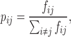(1)

where f_ij stands for the interaction frequency between ψ_i and ψ_j. Here, the neighboring affinity represents the probability that two genomic loci are neighbors. The neighborhood of a genomic locus thus can be featured by its neighboring affinities of this genomic locus. Here, we use the normalized interaction frequencies instead of the raw count information, which is more robust and happens to be the same as in t-SNE (33). Inspired by the idea of t-SNE, we map the Hi-C space representation of a chromosome, denoted by Ψ = {ψ₁, ψ₂, ⋅⋅⋅, ψ_n} (where n is the total number of genomic loci) into 3D Euclidean space to derive the final 3D chromatin structure, denoted by S = {s₁, s₂, ⋅⋅⋅, s_n}, where s_i represents the coordinates of the ith genomic locus in 3D Euclidean space, based on a neighboring affinity embedding process, which preserves the neighborhood information of genomic loci in Hi-C space as much as possible. That is, if two genomic loci are neighbor in Hi-C space, they would have a large probability of being neighbor in 3D Euclidean space.

In the t-SNE framework, which is a typical model of manifold learning, a Student t-distribution which generally has much heavier tails than Gaussian distribution is used to alleviate the ‘crowding problem’ (i.e., many close-by neighbors would be placed far off because of limited room when arranging high-dimensional data into low-dimensional space) in the embedding from high-dimensional to low-dimensional space (33). In our chromatin structure modeling problem, we use q_ij to denote the probability that genomic loci s_i and s_j pick each other as neighbors in 3D Euclidean space after embedding, which is defined as

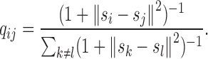(2)

where ‖ · ‖ stands for the Euclidean distance.

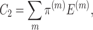
Chromatin can change dynamically in the nucleus especially during interphase. Thus, unlikely its structure can be accurately described by one single consensus conformation. In our framework, we develop a multi-conformation version of the embedding approach to model an ensemble of chromatin conformations. In particular, we use multiple 3D conformations with mixing proportions instead of a single conformation to interpret the Hi-C data. Here, we redefine the joint probability q_ij as

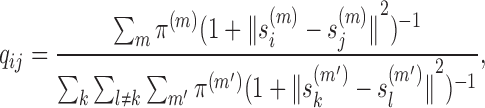(3)

where π^(m) stands for the mixing proportion of the m-th conformation, and 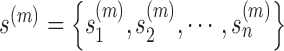represents the coordinates of the m-th conformation.

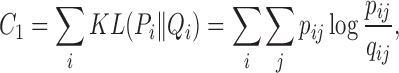
From the perspective of neighbor embedding (33,41), if an ensemble of chromatin conformations in 3D Euclidean space, denoted by {(s⁽¹⁾, π⁽¹⁾), (s⁽²⁾, π⁽²⁾), ⋅⋅⋅, (s^(m), π^(m))}, correctly models the neighborhood system of Ψ in Hi-C space, the joint probabilities p_ij and q_ij should match to each other. As in other t-SNE based learning tasks (42,43), we minimize the Kullback–Leibler (KL) divergence to find a low-dimensional (3D Euclidean space in our case) data representation that has the lowest degree of mismatch to the original Hi-C data (which can be considered in high-dimensional space). We use P_i to denote the neighborhood system of ψ_i in Hi-C space and Q_i to denote the neighborhood system of s_i in 3D Euclidean space. Moreover, we add a conformational energy term C₂ to ensure that the modeled structures have high energy stability. That is, the overall cost function C is defined as

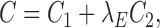(4)

(5)

(6)

where E^(m) stands for the conformational energy of the m-th conformation in the ensemble and λ_E stands for the coefficient that weighs the relative importance between the data term representing the fitness of Hi-C data and the energy term. More details about the optimization of the above cost function C can be found in Supplementary Methods.

Taking a deeper look at C₁, it is obvious that KL divergence is not symmetric (43). From a different perspective, represents a mismatch term and p_ij can be regarded as the weighting factor of such a mismatch term. This observation means that, there is a relatively large cost to use points far from each other (i.e. with small q_ij) in 3D Euclidean space to represent nearby genomic loci (i.e., with large p_ij) in Hi-C space, while it is of relatively small cost to use nearby points to represent two genomic loci far away in Hi-C space. In other words, GEM aims to preserve local structure when mapping from Hi-C space into 3D Euclidean space. This merit of retaining local structure particularly meets the requirement of 3D chromatin structure modeling, as Hi-C data exactly reflect the topological properties of local structures of chromosomes. In addition, it is reasonable to associate pairs of genomic loci with higher interaction frequencies with more confidence during the modeling process.

Inference of the relationships between Hi-C interaction frequencies and spatial distances

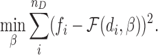
Once the chromatin structures are reconstructed, the distances between individual pairs of genomic loci can be determined. The zeros in the Hi-C interaction frequency matrix generally indicate missing or undetected values, and cannot be used to infer the relationships between Hi-C interaction frequencies and spatial distances. Thus, we only consider a set of the distances of the pairs of genomic loci whose Hi-C interaction frequencies are larger than zero, defined as D = {d_i, i = 1…n_D}, where n_D denotes the size of D. Suppose that the corresponding set of interaction frequencies of D is defined as F = {f_i, i = 1…n_D}. Then, we can perform curve fitting on data pairs {(d_i, f_i), i = 1…n_D} to derive a concrete function 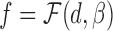that best describes the relationships between Hi-C interaction frequencies and spatial distances, where β denotes the parameters of the function model. To implement curve fitting, we optimize the nonlinear least-squares by the Trust-Region-Reflective Least Squares algorithm (44), that is,

(7)

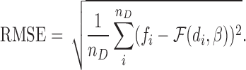
Also, the goodness of curve fitting is evaluated by the root-mean-square error (RMSE), that is,

(8)

In addition, we argue that making specific assumptions about the form of the relation function is not advisable, which is also validated in our experiment (Figure 5). Thus, here, the form of relation function is determined mainly based on the fitness to data which is measured by RMSE. Specifically, we use several common function forms (e.g., power model or gaussian model 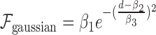) to fit the data and select the one with the lowest RMSE.

Figure 5.

Relationships between Hi-C interaction frequencies and reconstructed spatial distances derived based on different test settings of simulated Hi-C data. The purple curves depict the latent relationships between Hi-C interaction frequencies and reconstructed spatial distances derived based on the tests on simulated Hi-C data, which were generated according to different settings of the trapping rate α_t (A), the maximum interaction probability P_m (B), the standard deviation of Gaussian function σ (C), and the number of cells N_c (D), respectively. The blue, orange and green curves show the functions inferred by GEM, the hypothetical function F∝1/D used in the MDS (29,30) based model and ShRec3D (18), and the hypothetical function F∝1/D^α used in ChromSDE (17), respectively. The root-mean-square error (RMSE) was used to measure the distances between these functions used in the modeling frameworks (shown in blue, orange or green curves) and the latent functions (shown in purple curves), which can be derived from the parameter settings used to generate the simulated Hi-C data.

When the function is inferred as mentioned above, we can use it to back compute the interaction frequencies of the pairs of genomic loci whose Hi-C data are missing or undetected (i.e., the experimentally measured interaction frequencies are zero). Because the reconstructed chromatin structures include full spatial information of the whole chromosome, we can easily obtain the spatial distance of any pair of genomic loci whose Hi-C interaction frequency is missing or undetected and then apply on this distance to predict its Hi-C frequency.

RESULTS

Validation on simulated Hi-C data

We first validated the modeling performance of GEM on the simulated Hi-C data (see Supplementary Methods). The simulated Hi-C data were then fed into GEM to reconstruct the chromatin structures. We tested GEM on different simulated Hi-C maps which were generated by varying a wide range of parameter settings during the simulation process (Figure 2, Supplementary Figures S2–S4). Here, we evaluated the Pearson correlations between the distance matrices of our reconstructed models and the original conformations that were used to generate the simulated data. We also compared the modeling performance of GEM to that of three other reconstruction methods, including the MDS (29,30) based model, ChromSDE (17) and ShRec3D (18). As our simulation process did not consider the sequence content (e.g., GC content) of chromatin structures, here we did not include BACH (16) in the comparison tests on simulated Hi-C data. All the validation tests on synthetic Hi-C data generated by a variety of conditions showed that GEM achieved the best modeling performance in terms of the closeness to the original structures that were used to generate the simulated data (Figure 2A, Supplementary Figures S2A, S3A and S4A).

Figure 2.

The validation results on the simulated Hi-C data, which were generated according to different settings of the trapping rate α_t (see Supplementary Methods). (A) The comparisons of Pearson correlations between GEM and other modeling methods, including the MDS (29,30) based model, ChromSDE (17) and ShRec3D (18). (B and C) show the typical examples of the simulated Hi-C maps and the corresponding distributions of the simulated interaction frequencies as α_t increases, respectively. In the simulated Hi-C maps, the axes denote the genomic loci (1 Mb resolution) and the values of the entries indicate the simulated interaction frequencies. In the histograms, the x axes denote the interaction frequencies obtained from the Hi-C maps and the y axes denote the numbers of data points falling into individual interaction frequency intervals.

Validation on experimental Hi-C data

We then evaluated the modeling performance of GEM on experimental Hi-C data (7,14). We first used Pymol (45) to visualize the overall ensemble of the chromatin conformations reconstructed by GEM, taking human chromosome 14 at a resolution of 1 Mb as an example (Figure 3A). The modeled 3D organizations of chromosomes can provide a direct and vivid visualization about the 3D spatial arrangements of chromosomes, which may offer useful mechanistic insights about the 3D folding of chromatin structure and its functional roles in gene regulation. Through simple visual inspection of the ensemble of four chromatin conformations reconstructed by GEM (Figure 3A), we observed that they displayed similar but not identical 3D spatial organizations. In addition, we found that they are all organized into alike obvious isolated regions that agreed well with those identified from the Hi-C map. Such consistency of domain partition also suggested the reasonableness of the chromatin conformations reconstructed by GEM. Also, the similar domain partitions of different conformations were consistent with the previous studies (28,46,47) that topological domains are hallmarks of chromosomal conformations in spite of their dynamic structural variability.

Figure 3.

The chromatin structure modeling results on human chromosomes under 1 Mb resolution. (A) Visualization of the computed ensemble of human chromosome 14. The four conformations {s⁽¹⁾, s⁽²⁾, s⁽³⁾, s⁽⁴⁾} in the derived ensemble are shown in red, blue, green and orange, respectively. The middle shows the superimposition of all four conformations, which were all aligned using the singular value decomposition (SVD) algorithm (54). The three large isolated regions (α, β, γ) which can be facilely distinguished from the reconstructed 3D conformations were consistent well with those detected based on the original Hi-C map (see (C)). (B) The 10-fold cross-validation results for human chromosome 14, in which the scatter plot of the reconstructed Hi-C data derived from the modeled structures vs. the original Hi-C data is shown. (C, D) The original interaction frequency map derived from experimental Hi-C data and the reconstructed Hi-C map predicted by the modeled structures for human chromosome 14 in the 10-fold cross-validation results, respectively. In the Hi-C maps, the axes denote the genomic loci (1 Mb resolution) and the values of the entries indicate the experimentally measured (C) and predicted (D) interaction frequencies, respectively. (E) Bar graph depicting mutual validation by two sets of experimental Hi-C data for individual 23 human chromosomes, which were collected using two different restriction enzymes (i.e., HindIII vs. NcoI), respectively. (F, G) Comparison results between different modeling methods, in terms of the agreement between experimental and predicted Hi-C data and the conformational energy, respectively.

Next, we performed a 10-fold cross-validation procedure to assess the modeling performance of GEM on experimental Hi-C data (see Supplementary Methods). Our 10-fold cross-validation on human Hi-C data demonstrated that GEM was able to reconstruct accurate 3D chromatin structures that agreed well with the hold-out test data. For example, the predicted Hi-C data of human chromosome 14 inferred from the reconstructed conformations were consistent with the original experimental Hi-C data, with the Pearson correlation above 0.93 (Figure 3B–D).

We also conducted a mutual validation based on different Hi-C datasets collected from distinct experimental platforms. In particular, we chose two Hi-C datasets (7) that were collected using two different restriction enzymes (i.e., HindIII versus NcoI). These two datasets were fed into GEM separately and their modeling results were then evaluated by cross examining the correlations between the chromatin structures reconstructed from individual datasets. Such a mutual validation indicated that GEM was able to elucidate accurate chromatin structures that were consistent with the other independent dataset, achieving the Pearson correlations of distance matrices close or >0.8 (Figure 3E).

In the above cross-validation tests, we also compared the modeling results of GEM to those of other existing methods, including the the MDS (29,30) based model, BACH (16), ChromSDE (17) and ShRec3D (18). The comparisons demonstrated that GEM outperformed other four modeling methods, in terms of the Pearson correlation between the reconstructed interaction frequency data and the original experimental Hi-C data (Figure 3F and Supplementary Figure S5). Here, the reconstructed Hi-C maps for the other modeling methods were computed according to their hypothesis functions (MDS based model, ChromSDE and ShRec3D) or distributions (BACH) on the relationships between interaction frequencies and spatial distances between genomic loci. In addition, since our method also considered the conformational energy term during the modeling process, its reconstructed structures had significantly lower energy than those modeled by other four approaches (Figure 3G), which implied that GEM can yield biophysically more reasonable spatial representations of the observed Hi-C data.

Taken together, the above validation tests on experimental Hi-C data demonstrated that GEM can outperform other existing modeling methods, and reconstruct an ensemble of more accurate and biophysically more reasonable 3D organizations of chromosomes.

Validation on FISH data

In addition to the cross-validation tests on experimental Hi-C data, we also verified the modeled chromatin structures using a sparse set of known pairwise distance constraints between genomic loci driven by the FISH imaging techniques (Figure 4). In particular, we first examined the agreement between the chromatin structures reconstructed by GEM and the sparse FISH distance constraints obtained from the previously known studies (7,37,38), which included ARS603-ARS606, ARS606-ARS607, ARS607-ARS609 on yeast chromosome 6 and L1-L3, L2-L3, L2-L4 on human chromosome 14 (Figure 4). We compared the average distances between genomic loci driven from the FISH imaging data and our reconstructed models. In addition, we also analyzed the feasibility of the pairwise spatial distances between genomic loci predicted by GEM based on the relative sequence distances and corresponding compartmentalization information (7). On yeast chromosome 6 (Figure 4A), the reconstructed distance between ARS603 and ARS606 was relatively larger than those of other pairs, which was consistent with the fact that the pair ARS603-ARS606 crosses two different compartments (A and B), while the other two pairs (i.e., ARS606-ARS607 and ARS607-ARS609) are located within the same compartment (B). In the same compartment (B), the reconstructed distance between ARS606 and ARS607 was less than that between genomic loci ARS607 and ARS609, suggesting that a pair of genomic loci with small sequence distance preferentially stay close in space, which was also consistent with the previous studies (5,37). On human chromosome 14 (Figure 4B), the reconstructed distance between genomic loci L1 and L3 was notably smaller than that between L2 and L3, which agreed with the fact that, L2 and L3 are closer along the sequence but belong to different compartments (L2 in B and L3 in A), while L1 and L3 are further far away along the sequence but belong to the same compartment (A).

Figure 4.

The validation results on the known pairwise distance constraints derived from the FISH imaging data of yeast and human. (A) The validation results on the FISH imaging data of yeast chromosome 6. ARS603, ARS606, ARS607 and ARS609 lie consecutively along the chromosome. The genomic distance intervals of ARS603, ARS606, ARS607 and ARS609 are 103, 32 and 56 kb, respectively. ARS603 belongs to compartment A, while the other three loci belong to compartment B. (B) The validation results on the FISH imaging data of human chromosome 14. L1, L2, L3 and L4 lie consecutively along the chromosome. The genomic distance intervals of L1, L2, L3 and L4 are 23, 22 and 19 kb, respectively. L1 and L3 belong to compartment A, while L2 and L4 belong to compartment B. In (A) and (B), top shows the schematic illustrations of the locations of genomic loci used in the validation. Compartment partition was performed based on the eigenvectors of the Hi-C maps computed by principal component analysis (PCA) (7). Bottom shows the bar graphs depicting the comparisons between the mean distances between genomic loci derived from FISH imaging data and reconstructed by GEM. (C–E) The validation results on the FISH data (48) that include FISH distances between 34 TADs on human chromosome 21. (C) Visualization of the relative errors between the reconstructed distances by GEM and FISH distances, in which the axes denote the index of TADs and the values of the entries indicate the relative errors. (D) Comparison between different models in terms of relative errors between reconstructed spatial distances and FISH distances averaged over all pairs of TADs. (E) Red scatter plot shows the inverse Hi-C interaction frequencies between individual pairs of TADs versus their corresponding spatial distances derived from the FISH imaging data, while blue scatter plot shows the inverse Hi-C interaction frequencies between individual pairs of TADs versus their corresponding mean spatial distances computed by GEM.

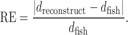
We also compared our reconstructed distances with the abundant FISH data derived from (48), which measured the spatial distances between all 34 TADs across human chromosome 21 in single cells (Figure 4C–E). We fed the corresponding 40 kb resolution Hi-C data (46) into GEM to reconstruct the chromosome structures and then computed the spatial distances between the centers of 34 TADs of the reconstructed structures, denoted by d_reconstruct. We used d_fish to denote the spatial distances derived from FISH between 34 TADs averaged across single cells, and then measured the relative error (RE) values, that is,

(9)

We visualized the relative errors for all pairs of TADs (Figure 4C) and also compared the average relative errors between different modeling methods (Figure 4D). GEM significantly outperformed MDS (29,30) based model, ChromSDE (17) and ShRec3D (18). More surprisingly, even without assuming any specific relationship between Hi-C interaction frequencies and spatial distances, our reconstructed distances still closely matched the scatter plot obtained from the FISH data (48) (Figure 4E).

Taken together, the above validation results showed that the chromatin structures modeled by GEM were in good agreement with the known pairwise distance constraints derived from FISH data in terms of both average spatial distances and compartment partition, which further verified the modeling power of our method.

Validation on modeling local topology

To test the competence of our framework in modeling local topology, we also ran GEM to reconstruct the structures of the ENCODE ENm008 region containing the α-globin locus on GM12878 cells and K562 cells, respectively. As shown in Supplementary Figure S7, the distance between the two ends of the modeled region (i.e. positions 55911–56690 and 402437–418222 on chromosome 16) was 0.4 folds shorter in GM12878 than in K562. It revealed that the compactness of this region in GM12878 was much smaller than K562, which was consistent with the previous reconstructed structures (10,26) and FISH data (10). Thus, GEM also works well for modeling local topology at the gene level.

Analysis of the relationships between Hi-C interaction frequencies and spatial distances

Here, we argued that the specific assumptions about the relationships between Hi-C interaction frequencies and spatial distances in most of previous chromatin structure modeling approaches are not advisable, based on our tests on the simulated Hi-C data, in which the true relationships between interaction frequencies and spatial distances were considered known and thus can be used to examine all possible hypothetical functions defining their relationships. First, the latent relationships between interaction frequencies and spatial distances can be affected by various factors and tend to display different concrete forms despite their similar inverse proportion forms. In addition, the relationships are generally complex and it is usually difficult to describe them by a consensus expression. As validated by the simulated Hi-C data (Figure 5), the latent functions between Hi-C interaction frequencies and spatial distances varied on the simulated Hi-C data generated according to different conditions. Moreover, many previous modeling approaches (14–18) mainly focused on the reciprocal forms (e.g. F∝1/D^α) between interaction frequencies and spatial distances and ignored the proportional factor. Thus, the final modeled structures were merely the scaled models of the true conformation conformations. To obtain the exact true structures, knowledge about the scaling factors was also required in these modeling methods. Here, GEM is able to reconstruct chromatin structures at the true scale by taking both the fitness of Hi-C data and the structure stability measured in terms of conformational energy into consideration during the embedding process.

By comparing the modeled structures with the original Hi-C data (as shown in the dashed box in Figure 1), GEM can also infer the latent relationships between interaction frequencies and spatial distances. We used the tests on simulated Hi-C data to demonstrate this point. Specifically, the plotted scatters between the simulated Hi-C interaction frequencies and the spatial distances derived from our modeled structures showed that there existed a certain function between them, which was roughly in a reciprocal form that had been widely accepted in the literature of chromatin structure modeling (7,15,49). We further estimated the latent functions in more detail by curve fitting into the scatter plots, which is implemented by finding the proper function forms and parameters with the lowest RMSEs (see Materials and Methods) to best interpret the scatters. The comparisons showed that our derived expressions were much closer to the real functions (which can be obtained from the simulated Hi-C data) between Hi-C interaction frequencies and spatial distances than the specific inverse proportion formulas assumed in the previous modeling approaches, including the MDS (29,30) based model, ShRec3D (18) and ChromSDE (17) (Figure 5). These results suggested that GEM can accurately capture the latent relationships between Hi-C interaction frequencies and spatial distances without making any specific assumption on the specific forms of their inverse proportion relationships during the structure modeling process.

Next, we analyzed the derived relationships between Hi-C interaction frequencies and spatial distances reconstructed by GEM on experimental Hi-C data (Figure 6). Indeed, there existed a certain inverse proportion function between the experimental Hi-C interaction frequencies and the reconstructed spatial distances, which can be confirmed by the goodness of the fitting results measured by the RMSEs. In addition, our investigation showed that chromatin structures from different chromosomes, at different resolutions or from different species can display distinct inverse proportion forms defining the relationships between Hi-C interaction frequencies and reconstructed spatial distances. This result further implied that it would be generally unadvisable to assume the existence of a single consensus expression for the relationships between Hi-C interaction frequencies and spatial distances between genomic loci.

Figure 6.

Relationships between Hi-C interaction frequencies and reconstructed spatial distances derived from the chromatin structures modeled by GEM on experimental Hi-C data. (A–D) The latent functions inferred by GEM between Hi-C interaction frequencies and reconstructed spatial distances on human chromosome 13 at 1Mb resolution, human chromosome 14 at 1Mb resolution, a 130Mb-180Mb region of human chromosome 1 at 250 kb resolution, and yeast chromosome 6 at 10 kb resolution, respectively. The functions were obtained by curve fitting to the points representing the pairs of Hi-C interaction frequencies and reconstructed spatial distances in the modeled structures. The expressions of the derived functions and the fitting results measured in terms of the root-mean-square errors (RMSEs) are also shown.

Application of the modeled chromatin structures to recover missing long-range genomic interactions

Most of previous studies mainly used the 3D chromatin structures reconstructed from Hi-C data to visualize and inspect the topological and spatial arrangements among different genomic regions (5,7,11–28). The modeled chromatin structures were rarely applied to expand the geometric constraints derived from the original experimental Hi-C data. On the other hand, due to experimental uncertainty, Hi-C data may miss a certain number of long-range genomic interactions or contain extra noisy spatial contacts between distal genomic loci. Nevertheless, the long-range spatial contacts derived from current Hi-C data are generally able to provide a sufficient number of geometric restraints to reconstruct accurate 3D scaffolds of chromosomes. In addition, the conformational energy incorporated in our modeling framework can provide an extra type of restraints to infer biophysically stable and reasonable chromatin structures. For example, conformational energy can provide useful information about the stretching and bending conditions of the chromatin fibres. Thus, the 3D chromatin scaffolds derived by GEM can provide accurate chromatin structure templates to recover those long-range genomic interactions that were missing in the original Hi-C map. This potential application can also be supported by the previous excellent validation results of GEM (Figure 3). For example, the 10-fold cross-validation results showed that the reconstructed Hi-C map inferred from the reconstructed conformations derived by GEM was consistent with the hold-out dataset in the original experimental data (Figure 3B–D), which basically indicated that the reconstructed structures can also be used to restore the missing long-range genomic interactions from the original input Hi-C data. Also, the additional validation tests on cross-platform Hi-C data demonstrated that the 3D chromatin conformations reconstructed by GEM from one Hi-C dataset can fit well into another independent dataset (Figure 3E).

We further used the tests on the Hi-C data (50) collected from different replicates or platforms to demonstrate the potential application of GEM in the recovery of the missing long-range genomic interactions in the original Hi-C map. We first fed the Hi-C data of one replicate into GEM and then used the Hi-C map from the other replicate to validate the missing loops indicated by the modeled chromatin structures. In particular, we looked into the fraction of missing distal chromatin loops that can be validated through another independent dataset. We found that the missing chromatin loops detected by GEM exhibited much closer spatial contacts than the background (i.e., all the reconstructed distances; rank sum test, P < 1 × 10⁻²³; Figure 7A and B). In addition, the distributions of the reconstructed distances of missing and known loops (which were present in the Hi-C data of current replicate) were actually close to each other, with the probability plot correlation coefficients >0.97 (Figure 7A and B). These observations imply that the missing chromatin loops in Hi-C maps can be potentially restored by the chromatin structures modeled by GEM.

Figure 7.

Application of the chromatin structures reconstructed by GEM into the recovery of missing long-range loops or contacts. (A, B) The recovery results on the missing loops on human chromosome 19 in the GM12878 cell line at 5 kb resolution from the Hi-C data of replicate 1 and replicate 2 (50), respectively. The orange curves represent the distributions of known loops (which were present in the Hi-C data of current replicate), while the blue curves represent the distributions of missing loops (which were missing in current replicate but present in the other replicate). The purple curves show the background distributions, i.e., the distributions of spatial distances in the reconstructed structures. The HiCCUPS algorithm (50) implemented in the Juicer tools (55), with 0.1% FDR, was used to call chromatin loops from Hi-C maps. (C–E) The recovery results on the missing promoter–promoter and promoter–enhancer contacts on human chromosome 19, using the chromatin structures reconstructed by GEM based on the promoter-other contacts derived from the capture Hi-C data (51). The purple curves show the background distributions, i.e. the distributions of all the reconstructed spatial distances (as in (A, B)), while the other curves represent the distributions of the promoter–promoter or promoter–enhancer contacts that were missing in the input promoter-other capture Hi-C data (51) but present in an independent Hi-C map (C), the promoter–promoter contacts derived from another capture Hi-C data (D), or the promoter–enhancer contacts identified by PSYCHIC (52) from an independent Hi-C map (50), all of which were also called the validation Hi-C data. In (C) and (D), the blue, orange and green curves represent the distributions of the top 5, 25 and 50 missing promoter–promoter contacts which had the highest interaction frequencies in the validation Hi-C data. In Panels (F), the blue curve represents the distribution of the missing promoter–enhancer contacts in the validation Hi-C data. (F, G) Two examples on the recovered promoter–enhancer (F) or promoter–promoter (G) contacts on human chromosome 19 of the GM12878 cell line that were recovered from the chromatin structures reconstructed by GEM from one Hi-C dataset and can be validated by another independent Hi-C dataset. The recovered loops are shown by orange linkers on the bottom, while the connected promoter and enhancers regions (which were annotated using the combination of ENCODE Segway (56) and ChromHMM (57) as in (58)) are shown in blue and green, respectively. Among the lists of chromatin features, H3K27 and DNase-seq signals indicate the active and accessibility states of both ends of chromatin loops, while the states of promoters and enhancers are marked by H3K4me3 and H3K4me1, respectively. All ChIP-seq and DNase-seq data were obtained from the ENCODE portal (59). The human reference genome GRCh38/hg38 was used.

We also applied the chromatin structures reconstructed by GEM to detect the missing promoter–promoter or promoter–enhancer contacts based on the promoter-other contact map derived from the capture Hi-C technique, a recently developed experimental method to identify promoter-containing chromosome interactions at the restriction fragment level (51). In capture Hi-C experiments, typically two types of long-range genomic interactions can be observed, i.e., promoter–promoter contacts and promoter-other contacts, depending on whether both ends of the DNA fragments are captured by the promoter regions in the genome. In general, the promoter-other contacts dominate the total number of the interaction frequencies detected by capture Hi-C. Here, we fed all the promoter-other contacts derived from the capture Hi-C data (51) into GEM, and then used the independent Hi-C datasets including conventional Hi-C data (50) and promoter–promoter contacts which were also derived from capture Hi-C experiments (51), to validate those missing long-range genomic contacts recovered by the reconstructed structures. Considering that the distal genomic contacts with more interaction frequencies in Hi-C maps tend to reflect the topological properties of genomic structures with more confidence, here we mainly examined the top 5, 25 and 50 missing promoter–promoter contacts with the highest interaction frequencies in the validation Hi-C data (Figure 7C and D). In addition, we used the promoter–enhancer contacts identified by PSYCHIC (52) from the conventional Hi-C data (50) to verify the missing distal contacts indicated from the reconstructed structures (Figure 7E). Our analysis results showed that these recovered promoter–promoter interactions displayed significantly shorter spatial distances than the background of all reconstructed spatial distances (Figure 7C–E; rank sum test, P < 5 × 10⁻⁴). These results indicated that GEM can be potentially applied to recover the missing long-range genomic interactions caused by the sparsity of the capture Hi-C data.

Careful examination of these missing loops indicated that they were of comparable biological importance to those known chromatin loops, and can also be well supported by the known evidence derived from available chromatin features. For example, the two missing chromatin loops involving promoter–enhancer and promoter–promoter interactions were also consistent with different epigenetic profiles, including chromatin accessibility and histone modification markers H3k27ac, H3k4me3 and H3k4me1 (Figure 7F and G). In addition, we observed a similar level of the enrichment of functional elements (e.g., H3K27ac, H3k4me3 and H3k4me1 signals, DNA accessible regions, annotated promoter and enhancer regions) in both missing and known chromatin loops (Supplementary Table S2). All these results also demonstrated that the chromatin conformations reconstructed by GEM can provide useful structural templates to recover those missing long-range genomic interactions from the original Hi-C data.

DISCUSSION

In this paper, we have developed a novel manifold learning based framework, called GEM, to reconstruct the 3D spatial organizations of chromosomes from Hi-C interaction frequency data. Under our framework, the 3D chromatin structures can be obtained by directly embedding the neighboring affinities from Hi-C space into 3D Euclidean space, and integrating both Hi-C data and conformational energy. Extensive validations on both simulated and experimental Hi-C data of yeast and human demonstrated that GEM can provide an accurate and robust modeling tool to derive a physically and physiologically reasonable 3D representations of chromosomes.

To our best knowledge, our work is the first attempt to exploit the chromatin structure modeling methods to recover long-range genomic interactions that are missing from original Hi-C data. Here, the ability to recover the missing long-range genomic interactions not only demonstrated a novel extended application of GEM but also provided a strong evidence corroborating the superiority of GEM in terms of physical and physiological reasonability.

Similar to many other computational methods for modeling 3D chromatin structures from interaction frequency data, GEM also faces several technical challenges, e.g., parameter selection and computational efficiency. In GEM, only one parameter (i.e., the coefficient of the energy term λ_E) need to be chosen for an input Hi-C dataset. It can be determined by an automatic parameter tuning method employed in our framework. In practice, due to the robustness of GEM, the default setting for this parameter often works well for most occasions, which can save the running time required in parameter selection. Considering that GEM takes a multi-conformation optimization strategy which is usually a time-consuming process, we suggest using a small number of conformations in the ensemble for those tasks with relatively large datasets (e.g., high-resolution Hi-C data) or applications that pay less attention to structural diversity of chromatin structures (e.g. recovery of missing long-range genomic interactions). In principle, more parallel computational schemes can also be employed to further accelerate the optimization process. When applying GEM to recover missing genomic interactions for high-resolution Hi-C and capture Hi-C data, we only demonstrated the distributions of the reconstructed spatial distances for those missing contacts (Figure 7). In the future, we will further extend GEM to infer the interaction counts of missing contacts under the scenario of extremely sparse Hi-C data.

DATA AVAILABILITY

The GEM model and the analysis data files can be downloaded from https://github.com/mlcb-thu/GEM. The Hi-C data of yeast can be downloaded from Duan et al. (14) (http://noble.gs.washington.edu/proj/yeast-architecture/sup.html). The Hi-C data of human used for model validation can be downloaded from NCBI GEO GSE18199 (7) and NCBI GEO GSE48262, and the normalized version can be downloaded from Yaffe et al. (53) (http://compgenomics.weizmann.ac.il/tanay/?page_id=283). The FISH data which measured the spatial distances between all 34 TADs across human chromosome 21 in single cells and the corresponding Hi-C data can be downloaded from www.sciencemag.org/cgi/content/full/science.aaf8084/DC1 and http://chromosome.sdsc.edu/mouse/hi-c/download.html, respectively. The Hi-C data and capture Hi-C data of human used for the recovery test are available in NCBI GEO GSE63525 and ArrayExpress E-MTAB-2323, respectively.

SUPPLEMENTARY DATA

Supplementary Data are available at NAR Online.

FUNDING

National Natural Science Foundation of China [61472205, 81630103]; China’s Youth 1000-Talent Program; Beijing Advanced Innovation Center for Structural Biology; NCSA Faculty fellowship 2017; Israeli Center of Excellence (I-CORE) for Chromatin and RNA in Gene Regulation [1796/12]; Israel Science Foundation [913/15]. T.K. is a member of the Israeli Center of Excellence (I-CORE) for Gene Regulation in Complex Human Disease [41/11]. J.P. is funded by a Sloan Research Fellowship and NSF Career Award 1652815. Funding for open access charge: China’s Youth 1000-Talent Program.

Conflict of interest statement. None declared.

REFERENCES

- 1. de Laat W., Grosveld F.. Spatial organization of gene expression: the active chromatin hub. Chromosome Res. 2003; 11:447–459. [DOI] [PubMed] [Google Scholar]
- 2. Fraser P., Bickmore W.. Nuclear organization of the genome and the potential for gene regulation. Nature. 2007; 447:413–417. [DOI] [PubMed] [Google Scholar]
- 3. Cremer T., Cremer C.. Chromosome territories, nuclear architecture and gene regulation in mammalian cells. Nat. Rev. Genet. 2001; 2:292–301. [DOI] [PubMed] [Google Scholar]
- 4. Misteli T. Beyond the sequence: cellular organization of genome function. Cell. 2007; 128:787–800. [DOI] [PubMed] [Google Scholar]
- 5. Dekker J., Rippe K., Dekker M., Kleckner N.. Capturing chromosome conformation. Science. 2002; 295:1306–1311. [DOI] [PubMed] [Google Scholar]
- 6. Schmitt A.D., Hu M., Ren B.. Genome-wide mapping and analysis of chromosome architecture. Nat. Rev. Mol. Cell Biol. 2016; 17:743–755. [DOI] [PMC free article] [PubMed] [Google Scholar]
- 7. Lieberman-Aiden E., Van Berkum N.L., Williams L., Imakaev M., Ragoczy T., Telling A., Amit I., Lajoie B.R., Sabo P.J., Dorschner M.O. et al. Comprehensive mapping of long-range interactions reveals folding principles of the human genome. Science. 2009; 326:289–293. [DOI] [PMC free article] [PubMed] [Google Scholar]
- 8. Li G., Fullwood M.J., Xu H., Mulawadi F.H., Velkov S., Vega V., Ariyaratne P.N., Mohamed Y.B., Ooi H.-S., Tennakoon C. et al. ChIA-PET tool for comprehensive chromatin interaction analysis with paired-end tag sequencing. Genome Biol. 2010; 11:R22. [DOI] [PMC free article] [PubMed] [Google Scholar]
- 9. Kalhor R., Tjong H., Jayathilaka N., Alber F., Chen L.. Genome architectures revealed by tethered chromosome conformation capture and population-based modeling. Nat. Biotechnol. 2012; 30:90–98. [DOI] [PMC free article] [PubMed] [Google Scholar]
- 10. Baù D., Sanyal A., Lajoie B.R., Capriotti E., Byron M., Lawrence J.B., Dekker J., Marti-Renom M.A.. The three-dimensional folding of the α-globin gene domain reveals formation of chromatin globules. Nat. Struct. Mol. Biol. 2011; 18:107–114. [DOI] [PMC free article] [PubMed] [Google Scholar]
- 11. Ay F., Noble W.S.. Analysis methods for studying the 3D architecture of the genome. Genome Biol. 2015; 16:183. [DOI] [PMC free article] [PubMed] [Google Scholar]
- 12. Tjong H., Gong K., Chen L., Alber F.. Physical tethering and volume exclusion determine higher-order genome organization in budding yeast. Genome Res. 2012; 22:1295–1305. [DOI] [PMC free article] [PubMed] [Google Scholar]
- 13. Varoquaux N., Ay F., Noble W.S., Vert J.-P.. A statistical approach for inferring the 3D structure of the genome. Bioinformatics. 2014; 30:i26–i33. [DOI] [PMC free article] [PubMed] [Google Scholar]
- 14. Duan Z., Andronescu M., Schutz K., McIlwain S., Kim Y.J., Lee C., Shendure J., Fields S., Blau C.A., Noble W.S.. A three-dimensional model of the yeast genome. Nature. 2010; 465:363–367. [DOI] [PMC free article] [PubMed] [Google Scholar]
- 15. Rousseau M., Fraser J., Ferraiuolo M.A., Dostie J., Blanchette M.. Three-dimensional modeling of chromatin structure from interaction frequency data using Markov chain Monte Carlo sampling. BMC Bioinformatics. 2011; 12:414. [DOI] [PMC free article] [PubMed] [Google Scholar]
- 16. Hu M., Deng K., Qin Z., Dixon J., Selvaraj S., Fang J., Ren B., Liu J.S.. Bayesian inference of spatial organizations of chromosomes. PLoS Comput. Biol. 2013; 9:e1002893. [DOI] [PMC free article] [PubMed] [Google Scholar]
- 17. Zhang Z., Li G., Toh K.-C., Sung W.-K.. 3D chromosome modeling with semi-definite programming and Hi-C data. J. Comput. Biol. 2013; 20:831–846. [DOI] [PubMed] [Google Scholar]
- 18. Lesne A., Riposo J., Roger P., Cournac A., Mozziconacci J.. 3D genome reconstruction from chromosomal contacts. Nat. Methods. 2014; 11:1141–1143. [DOI] [PubMed] [Google Scholar]
- 19. Wang S., Xu J., Zeng J.. Inferential modeling of 3D chromatin structure. Nucleic Acids Res. 2015; 43:e54. [DOI] [PMC free article] [PubMed] [Google Scholar]
- 20. Trussart M., Serra F., Baù D., Junier I., Serrano L., Marti-Renom M.A.. Assessing the limits of restraint-based 3D modeling of genomes and genomic domains. Nucleic Acids Res. 2015; 43:3465–3477. [DOI] [PMC free article] [PubMed] [Google Scholar]
- 21. Carstens S., Nilges M., Habeck M.. Inferential structure determination of chromosomes from single-cell Hi-C data. PLOS Comput. Biol. 2016; 12:e1005292. [DOI] [PMC free article] [PubMed] [Google Scholar]
- 22. Park J., Lin S.. Impact of data resolution on three-dimensional structure inference methods. BMC Bioinformatics. 2016; 17:70. [DOI] [PMC free article] [PubMed] [Google Scholar]
- 23. Zou C., Zhang Y., Ouyang Z.. HSA: integrating multi-track Hi-C data for genome-scale reconstruction of 3D chromatin structure. Genome Biol. 2016; 17:40. [DOI] [PMC free article] [PubMed] [Google Scholar]
- 24. Adhikari B., Trieu T., Cheng J.. Chromosome3D: reconstructing three-dimensional chromosomal structures from Hi-C interaction frequency data using distance geometry simulated annealing. BMC Genomics. 2016; 17:886. [DOI] [PMC free article] [PubMed] [Google Scholar]
- 25. Tjong H., Li W., Kalhor R., Dai C., Hao S., Gong K., Zhou Y., Li H., Zhou X.J., Le Gros M.A. et al. Population-based 3D genome structure analysis reveals driving forces in spatial genome organization. Proc. Natl. Acad. Sci. U.S.A. 2016; 113:E1663–E1672. [DOI] [PMC free article] [PubMed] [Google Scholar]
- 26. Paulsen J., Sekelja M., Oldenburg A.R., Barateau A., Briand N., Delbarre E., Shah A., Sørensen A.L., Vigouroux C., Buendia B. et al. Chrom3D: three-dimensional genome modeling from Hi-C and nuclear lamin-genome contacts. Genome Biol. 2017; 18:21. [DOI] [PMC free article] [PubMed] [Google Scholar]
- 27. Rieber L., Mahony S.. miniMDS: 3D structural inference from high-resolution Hi-C data. Bioinformatics. 2017; 33:i261–i266. [DOI] [PMC free article] [PubMed] [Google Scholar]
- 28. Nagano T., Lubling Y., Stevens T.J., Schoenfelder S., Yaffe E., Dean W., Laue E.D., Tanay A., Fraser P.. Single-cell Hi-C reveals cell-to-cell variability in chromosome structure. Nature. 2013; 502:59–64. [DOI] [PMC free article] [PubMed] [Google Scholar]
- 29. Torgerson W.S. Multidimensional scaling: I. Theory and method. Psychometrika. 1952; 17:401–419. [Google Scholar]
- 30. Young G., Householder A.S.. Discussion of a set of points in terms of their mutual distances. Psychometrika. 1938; 3:19–22. [Google Scholar]
- 31. Borg I., Groenen P.J.. Modern Multidimensional Scaling: Theory and Applications. 2005; Springer Science & Business Media. [Google Scholar]
- 32. Stevens T.J., Lando D., Basu S., Atkinson L.P., Cao Y., Lee S.F., Leeb M., Wohlfahrt K.J., Boucher W., O’Shaughnessy-Kirwan A. et al. 3D structures of individual mammalian genomes studied by single-cell Hi-C. Nature. 2017; 544:59–64. [DOI] [PMC free article] [PubMed] [Google Scholar]
- 33. Maaten L. v.d., Hinton G.. Visualizing data using t-SNE. J. Mach. Learn. Res. 2008; 9:2579–2605. [Google Scholar]
- 34. Lee J.A., Verleysen M.. Nonlinear Dimensionality Reduction. 2007; Springer Science & Business Media. [Google Scholar]
- 35. Tenenbaum J.B., De Silva V., Langford J.C.. A global geometric framework for nonlinear dimensionality reduction. science. 2000; 290:2319–2323. [DOI] [PubMed] [Google Scholar]
- 36. Lawrence N.D. A unifying probabilistic perspective for spectral dimensionality reduction: Insights and new models. J. Mach. Learn. Res. 2012; 13:1609–1638. [Google Scholar]
- 37. Bystricky K., Heun P., Gehlen L., Langowski J., Gasser S.M.. Long-range compaction and flexibility of interphase chromatin in budding yeast analyzed by high-resolution imaging techniques. Proc. Natl. Acad. Sci. U.S.A. 2004; 101:16495–16500. [DOI] [PMC free article] [PubMed] [Google Scholar]
- 38. Miele A., Bystricky K., Dekker J.. Yeast silent mating type loci form heterochromatic clusters through silencer protein-dependent long-range interactions. PLoS Genet. 2009; 5:e1000478. [DOI] [PMC free article] [PubMed] [Google Scholar]
- 39. Lanctôt C., Cheutin T., Cremer M., Cavalli G., Cremer T.. Dynamic genome architecture in the nuclear space: regulation of gene expression in three dimensions. Nat. Rev. Genet. 2007; 8:104–115. [DOI] [PubMed] [Google Scholar]
- 40. Osborne C.S., Chakalova L., Mitchell J.A., Horton A., Wood A.L., Bolland D.J., Corcoran A.E., Fraser P.. Myc dynamically and preferentially relocates to a transcription factory occupied by Igh. PLoS Biol. 2007; 5:e192. [DOI] [PMC free article] [PubMed] [Google Scholar]
- 41. Hinton G., Roweis S.. Stochastic neighbor embedding. NIPS. 2002; 15:833–840. [Google Scholar]
- 42. Van der Maaten L., Hinton G.. Visualizing non-metric similarities in multiple maps. Mach. Learn. 2012; 87:33–55. [Google Scholar]
- 43. Cook J., Sutskever I., Mnih A., Hinton G.E.. Visualizing similarity data with a mixture of Maps. AISTATS. 2007; 7:67–74. [Google Scholar]
- 44. Moré J.J., Sorensen D.C.. Computing a trust region step. SIAM J. Scientific Stat. Comput. 1983; 4:553–572. [Google Scholar]
- 45. Schrödinger, LLC The PyMOL Molecular Graphics System. 2015; Version 1.8. [Google Scholar]
- 46. Dixon J.R., Selvaraj S., Yue F., Kim A., Li Y., Shen Y., Hu M., Liu J.S., Ren B.. Topological domains in mammalian genomes identified by analysis of chromatin interactions. Nature. 2012; 485:376–380. [DOI] [PMC free article] [PubMed] [Google Scholar]
- 47. Dixon J.R., Gorkin D.U., Ren B.. Chromatin domains: the unit of chromosome organization. Mol. Cell. 2016; 62:668–680. [DOI] [PMC free article] [PubMed] [Google Scholar]
- 48. Wang S., Su J.-H., Beliveau B.J., Bintu B., Moffitt J.R., Wu C.-t., Zhuang X.. Spatial organization of chromatin domains and compartments in single chromosomes. Science. 2016; 353:598–602. [DOI] [PMC free article] [PubMed] [Google Scholar]
- 49. Fraser J., Rousseau M., Shenker S., Ferraiuolo M.A., Hayashizaki Y., Blanchette M., Dostie J.. Chromatin conformation signatures of cellular differentiation. Genome Biol. 2009; 10:R37. [DOI] [PMC free article] [PubMed] [Google Scholar]
- 50. Rao S.S., Huntley M.H., Durand N.C., Stamenova E.K., Bochkov I.D., Robinson J.T., Sanborn A.L., Machol I., Omer A.D., Lander E.S. et al. A 3D map of the human genome at kilobase resolution reveals principles of chromatin looping. Cell. 2014; 159:1665–1680. [DOI] [PMC free article] [PubMed] [Google Scholar]
- 51. Mifsud B., Tavares-Cadete F., Young A.N., Sugar R., Schoenfelder S., Ferreira L., Wingett S.W., Andrews S., Grey W., Ewels P.A. et al. Mapping long-range promoter contacts in human cells with high-resolution capture Hi-C. Nat. Genet. 2015; 47:598–606. [DOI] [PubMed] [Google Scholar]
- 52. Ron G., Globerson Y., Moran D., Kaplan T.. promoter–enhancer Interactions Identified from Hi-C Data using Probabilistic Models and Hierarchical Topological Domains. Nature communications. 2017; 8:2237. [DOI] [PMC free article] [PubMed] [Google Scholar]
- 53. Yaffe E., Tanay A.. Probabilistic modeling of Hi-C contact maps eliminates systematic biases to characterize global chromosomal architecture. Nat. Genet. 2011; 43:1059–1065. [DOI] [PubMed] [Google Scholar]
- 54. Sorkine O. Least-squares rigid motion using svd. Technical notes. 2009; 120:52. [Google Scholar]
- 55. Durand N.C., Shamim M.S., Machol I., Rao S.S., Huntley M.H., Lander E.S., Aiden E.L.. Juicer provides a one-click system for analyzing loop-resolution Hi-C experiments. Cell Syst. 2016; 3:95–98. [DOI] [PMC free article] [PubMed] [Google Scholar]
- 56. Hoffman M.M., Buske O.J., Wang J., Weng Z., Bilmes J.A., Noble W.S.. Unsupervised pattern discovery in human chromatin structure through genomic segmentation. Nat. Methods. 2012; 9:473–476. [DOI] [PMC free article] [PubMed] [Google Scholar]
- 57. Ernst J., Kellis M.. ChromHMM: automating chromatin-state discovery and characterization. Nat. Methods. 2012; 9:215–216. [DOI] [PMC free article] [PubMed] [Google Scholar]
- 58. Whalen S., Truty R.M., Pollard K.S.. Enhancer-promoter interactions are encoded by complex genomic signatures on looping chromatin. Nat. Genet. 2016; 48:488–496. [DOI] [PMC free article] [PubMed] [Google Scholar]
- 59. ENCODE Project Consortium An integrated encyclopedia of DNA elements in the human genome. Nature. 2012; 489:57–74. [DOI] [PMC free article] [PubMed] [Google Scholar]
Associated Data
This section collects any data citations, data availability statements, or supplementary materials included in this article.
Supplementary Materials
Data Availability Statement