EHR-Based Phenotyping: Bulk Learning and Evaluation

Abstract

In data-driven phenotyping, a core computational task is to identify medical concepts and their variations from sources of electronic health records (EHR) to stratify phenotypic cohorts. A conventional analytic framework for phenotyping largely uses a manual knowledge engineering approach or a supervised learning approach where clinical cases are represented by variables encompassing diagnoses, medicinal treatments and laboratory tests, among others. In such a framework, tasks associated with feature engineering and data annotation remain a tedious and expensive exercise, resulting in poor scalability. In addition, certain clinical conditions, such as those that are rare and acute in nature, may never accumulate sufficient data over time, which poses a challenge to establishing accurate and informative statistical models. In this paper, we use infectious diseases as the domain of study to demonstrate a hierarchical learning method based on ensemble learning that attempts to address these issues through feature abstraction. We use a sparse annotation set to train and evaluate many phenotypes at once, which we call bulk learning. In this batch-phenotyping framework, disease cohort definitions can be learned from within the abstract feature space established by using multiple diseases as a substrate and diagnostic codes as surrogates. In particular, using surrogate labels for model training renders possible its subsequent evaluation using only a sparse annotated sample. Moreover, statistical models can be trained and evaluated, using the same sparse annotation, from within the abstract feature space of low dimensionality that encapsulates the shared clinical traits of these target diseases, collectively referred to as the bulk learning set.

1. Introduction

Predictive analytics using EHR data has gone through tremendous advancement over the past few years owing to the emergence of large-scale data integration such as the clinical data warehouse (CDR). In particular, population-scale clinical data that incorporate patient diagnoses, tests, and medical history, among many others, are essential to computational phenotyping for which the primary objective is to define disease-specific cohorts and unravel potential disease subtypes [1–3].

In the general landscape of computational phenotyping research, many endeavors have been made to progressively replace the predominant use of rule-based phenotyping algorithms, comprising the majority in eMERGE network [4], by the predictive analytical approach based on machine learning and natural language processing (NLP) [5–8]. While this data-driven analytic methodology alleviates the tedious process of manually selecting features and their logical combinations that match phenotype definitions in an ad hoc fashion, predictive analytics is not without its own outstanding challenges. In particular, during the creation of training data, both feature engineering and data labeling involve significant human interventions as a prerequisite for applying machine learning algorithms, which on many levels is the reason that labeled data are still relatively limited as a resource for large-scale or high-throughput phenotyping effort. Wilcox et al. showed that experts were better off putting their time into rule authoring than training set annotation [9]. As a vantage point for predictive modeling, nonetheless, EHR is data-rich in clinical details including disease diagnoses and treatments as well as a gradual integration of genomic data for precision medicine.

In this study, we focus on developing a clean, flexible algorithmic approach towards batch-phenotyping multiple diseases with minimal intervention of clinical experts. Specifically, we focus on the computational phenotyping of infectious diseases as the domain of study given that this disease class has the following characteristics. Firstly, the etiology of infectious diseases is complex due to a wide spectrum of pathogenic microbes, some of which can even cause several diseases; additionally, pathological factors such as sites of infections, and immune system responses further add to the etiological complexity, making the task of data annotation inherently challenging. Secondly, a significant portion of the infectious diseases has ambiguous classifications (e.g. unspecified bacterial infections, 041.9) in the ICD-9-CM system. Moreover, while common infectious diseases have sufficient data points for establishing predictive models, relatively rare infections may always be short of data. For instance, infectious diseases with demographically rare occurrences such as anthrax and the emerging infections would inherently accumulate smaller data sets than those of the pandemic conditions such as influenza and chronic, prolonged conditions such as hepatitis-B.

With the help of diagnostic codes, we postulate that predictive models for rare infectious disease cases can be built on top of those more frequently observed assuming that there exist overlapping clinical elements that can reasonably distinguish infectious conditions from one another. More concretely, we adopt an algorithmic design based on the ensemble learning in the form of stacked generalization [10–13], which when combined with ontological feature selection, gives rise to levels of feature abstraction that helps to delineate phenotypic boundaries over multiple infectious diseases in parallel.

To reinforce the aspect of the simultaneous model learning over multiple clinical conditions, we refer to this batch-phenotyping method as bulk learning. In particular, feature abstractions in the learning hierarchy allow for statistical models to be established in an (abstract) feature space of low dimensionality, which lends itself to a more efficient and scalable training and evaluation with lessened requirement of labeled data in addition to interpretable modeling results. In the experiment, we use a small annotation set comprising randomly sampled clinical cases of infectious diseases of interest to empirically demonstrate its capacity towards evaluating the predictive performance of the bulk learning system.

2. Materials and Methods

2.1 Overview

Phenotyping on a per-disease basis can be slow and is subject to the availability of the patient data for training accurate models. Bulk learning, as the name suggests, is a simultaneous learning and phenotyping procedure for multiple clinical conditions. The central idea is to use diagnostic codes, such as ICD-9-CM, readily available in the codified EHR data, as surrogate labels and train an intermediate model based on feature abstractions that capture clinical concepts shared among the set of clinical conditions. Disease labeling can then be achieved through the learned feature abstraction that enables a reduction of manually labeled data required for stratifying cohorts associated with each condition in the set. In this study, we use the clinical data repository (CDR) from the collaborative effort between Columbia University Medical Center and NewYork-Presbyterian Hospital and examine 100 clinically different infectious diseases in the CDR from the cohort identified from year 1985 to year 2014.

As we shall see shortly, each infectious disease in the bulk learning set is to be modeled by multiple classifiers, each of which corresponds to a clinical concept defined via a medical ontology. The training procedure consists of three stages, which manifest themselves through a hierarchical learning architecture. In the first stage, base classifiers are trained to predict labels of the set of the infectious diseases where the labels are identified via using ICD-9 codes as surrogates. In particular, the labels are “noisy” since the diagnostic coding system was created mainly for administrative and billing purposes and hence not always accurate [14,15]. Fig. 1 illustrates a high-level view of a three-tier model stacking. In the second stage, predictions from these base classifiers are aggregated through a meta-classifier, which gives rise to a feature abstraction that tells us the degree to which each base model contributes to the prediction for a given disease. In particular, the outputs from the lower tier such as probability scores in turn serve as abstract features in the upper tier. Subsequently in the third stage, we select a small subset of disease cases from which to create an annotation set with the erroneous diagnostic coding rectified by manual curation.

Fig. 1.

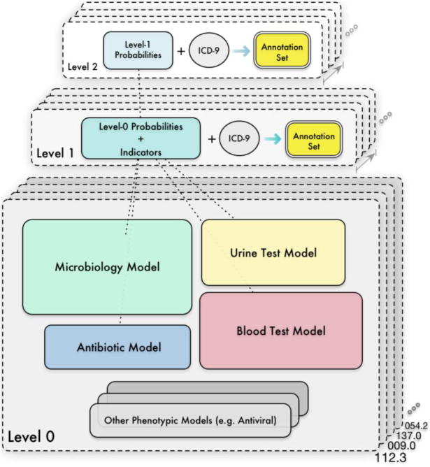
An example bulk learning hierarchy comprising two levels of feature abstractions over 4 phenotypic models.

As we shall see later, there are design choices associated with the abstract feature representations, which can influence model performance. The main objective of bulk learning is therefore to separate the disease cohorts with minimal data annotation effort by establishing statistical models from within the abstract feature space of low sample complexity that serves as a compact representation for the raw feature space spanned by patient attributes extracted from the EHR data.

2.2 Training Data Formulation and Data Characteristics

2.2.1 Bulk Learning Set

The set of candidate infectious diseases to be included in the bulk learning system can be identified via mentions of diagnostic codes, such as ICD-9, in the EHR data. In the CDR, each clinical visit is associated with a diagnostic entry, which typically has mentions of ICD-9 codes in three different categories: admission, primary and secondary diagnosis and more often than not, codes in these slots are not consistent. In this study, we only examine the primary and secondary diagnoses with better coding accuracy. There are approximately 1500 diagnostic codes found in CDR that fall in the category of infectious diseases, out of which we selected 100 codes to form the bulk learning set. Table 1 illustrates the bulk learning set under the classification of the ICD-9 coding in the section of infectious and parasitic diseases with an exception of 481, which falls in the category of pneumonia and influenza. To simplify the assumption for the purpose of illustrating bulk learning, different ICD-9 codes are considered as representing different diseases. The strategy of selecting diseases for bulk learning can influence the experimental results, for which further details can be found in the online supplement (Section A).

Table 1.

Infectious diseases in the bulk learning set stratified by categories according to the ICD-9 classification.

ICD-9 Classification	Bulk Learning Set	Count
Intestinal infectious diseases (001-009)	001.1, 003.0, 005.9, 007.1, 008.45, 008.61, 008.69, 009.0, 009.1, 009.3	10
Tuberculosis (010-018)	010.10, 011.93, 017.00	3
Zoonotic bacterial diseases (020-027)	027.0	1
Other bacterial diseases (030-041)	031.0, 031.2, 031.8, 031.9, 033.9, 034.0, 036.0, 038.10, 038.11, 038.19, 038.40, 038.42, 038.8, 040.82, 041.00, 041.09, 041.10, 041.11, 041.6, 041.7, 041.85, 041.89, 041.9	23
HIV infection (042-044)	n/a	0
Poliomyelitis & other non-arthropod-borne viral diseases of central nervous system (045-049)	046.3, 047.8, 047.9, 049.9	4
Viral diseases accompanies by exanthem (050-059)	052.7, 053.19, 053.79, 053.9, 054.10, 054.11, 054.13, 054.19, 054.2, 054.3, 054.79, 057.9	12
Arthropod-borne viral diseases (060-066)	061	1
Other diseases duo to viruses & chlamydiae (070-079)	070.30, 070.32, 070.51, 070.70, 070.71, 075, 078.0, 078.5, 079.0, 079.4, 079.6	11
Rickettsioses & other arthropod-borne diseases (080-088)	083.2, 087.9, 088.81	3
Syphilis & other venereal diseases (090-099)	090.1, 090.9, 091.3, 094.9, 097.1, 097.9, 098.0, 099.9	8
Other spirochetal diseases (100-014)	n/a	0
Mycoses (110-118)	110.0, 110.3, 111.9, 112.2, 112.3, 112.4, 112.5, 112.84, 112.89, 117.3, 117.5, 117.9	12
Helminthiases (120-129)	123.1, 127.4	2
Other infectious & parasitic diseases (130-136)	130.0, 130.7, 131.01, 133.0, 135, 136.3, 136.9	7
Late effects of infectious diseases (137-139)	137.0, 138	2
Pneumonia & Influenza (480-488)	481	1

2.2.2 Representing Clinical Cases

The process of formulating and collecting training data depends on how clinical cases are represented. In light of common practices in supervised learning, all training instances typically share the same feature set (e.g. clinical variables relevant for predicting disease cohorts). However problems arise when the feature set becomes large, which inevitably leads to a demanding effort in creating labeled data. A common way to address this issue is to employ dimensionality reduction techniques either via feature transformation (e.g. [16]) or feature subset selection (e.g. [17,18]). The design choice between these two lines of approach depends on the clinical utility that one seeks. In computational phenotyping, it is beneficial to obtain easily interpretable results as byproducts in addition to accurate predictive modeling. In particular, from the perspective of phenotypic concept discovery, a feature transformation using commonly used optimization objectives, such as the linear combination of features that accounts for the most data variance in PCA, may not immediately result in transformed features with clear clinical meanings. Feature subset selection on the other hand helps to identify informative variables in the statistical sense that contribute the most to the prediction. However, arbitrarily discarding less predictive variables is not satisfactory since clinical variables are often correlated and need to coexist to have clinical meanings¹. Popular statistical methods that identify correlated variables include ElasticNet [19], group lasso [20], etc. Yet, such data-driven group feature selection is highly contingent upon clinical data characteristics, which may not generalize well across multiple institutions; in particular, without sufficient data in clinical cases, the group correlations with a given target disease may not be significant enough to be identified.

For the purpose of disease phenotyping, we choose to represent cases in a hierarchical and modular form through the medical ontology, which has a clearly defined concept hierarchy and thereby facilitates the process of feature engineering. As we shall see in Section 2.3, grouping clinical variables via the medical ontology helps to break down the potentially large raw feature set, identified from the CDR, into several conceptual groups so that statistical models can be trained based on only the smaller group features at the base level. Through the ontology-based feature decomposition, clinical cases can assume a representation that is clearly defined, multifaceted and easily extensible. For instance, the same clinical case can be interpreted from the angle of the medicinal treatment and the laboratory test, among many others.

2.2.3 Data Preparation

To formulate a training set that takes the form of the patient representation given earlier, we first single out, from the CDR, the patient records tied to each target ICD-9 code documented in primary and secondary diagnosis followed by cross-referencing these records with the tables hosting the data for the clinical concepts of interest. In particular, we look for the clinical records that fall within the range of 60 days prior to the mention of a target ICD-9 code and 30 days following the mention. We note that tolerable errors in time shall be considered as adjustable parameters, when appropriate, that depend on the clinical practices.

As we shall see in Section 2.3, training data for bulk learning are concept-specific (i.e. each base model has its own training sets) and hence their feature representations depend on the concept hierarchy of the chosen medical ontology. Training data are collected via matching variables between those delineated by the concept hierarchy and patient attributes embedded within the aforementioned records, grouped by ICD-9 codes as surrogate labels, assuming that patient attributes had been codified to be consistent with the ontology.

2.2.4 Control Groups

In bulk learning, each predictive unit is formulated as a binary classification problem such as each disease-specific binary classifier at the base level and hence is associated with both positive and negative examples. While positive examples are created via referencing the diagnostic code, negative examples on the other hand are created via mixing different control data sets, which can be derived from different infectious disease cohorts or even from clinical cases without any infections involved. As the control data can greatly impact the chance of finding clinically meaningful predictors for a target disease, we ensure that the set of features in use by at least some training instances are reasonably similar to each other in both class labels.

For ease of exposition, we start with a few definitions. First, we define shared variables as the predictor variables that not only occur in the training instances of both class labels but also assume non-trivial values, where the non-triviality depends on the domain of the variable and its meanings. The assumption made in this study is simply that a value of 0 signifies a non-event (and hence trivial) whereas any non-zero values signify a triggered event (e.g. ruling out an organism as the cause of infection) or an observed measurement (e.g. intravenous chemistry). When a variable assumes a non-trivial value, it is referred to as an active variable. Thus, the set of shared variables can be determined by those that are active in at least m training instances of both class labels (where m=1 in this study). Furthermore, since a training set can consist of an arbitrary number of instances, it is useful to rank active variables in terms of the frequency of active occurrences; i.e. the number of times that a variable assumes an active state in the training data.

In order to match the positive and negative cases in a manner that maximizes the number of their shared variables, we use Jaccard coefficient to quantify the similarity of active variables between any pairs of training sets with one representing the target disease and the other representing the control. For computational efficiency, each training set is represented by a set of frequently active variables, top 80% in their active occurrences, which expresses a global characteristic of the underlying sample and simplifies similarity computations. In this manner, we choose, for each target disease, the top three most similar training sets, as the control data, from any of the non-target diseases in the bulk learning set.

2.3 Phenotypic Groups and Feature Abstraction

Infectious diseases exhibit a wide range of data distributions in EHR – some diagnostic codes have a few tens of thousands of patient records, especially those with ambiguous classification, while others may only have a few to no data points. A key step towards transcending the modeling dependency on varying sample sizes within the bulk learning set is to identify common, high-level clinical concepts that can reasonably stratify disease-specific cohorts and better yet, generalize across diseases, particular those with insufficient data. In this study, a clinical concept is defined as a group of closely related variables attributable to a phenotype from the perspective of clinical records; in particular, a phenotype, typically referring to a disease or its subtypes [21–23], is regarded as a collection of laboratory measurements, medicinal treatments, etc., that defines a concept-driven disease cohort².

2.3.1 Ontological Feature Representation for Clinical Cases

Ontology-driven feature engineering can be motivated from the clinical commonality observed within the diagnoses and treatments of diseases historically known as being different. In the study of neuropsychiatric disorders from EHR [22], for instance, phenotypic overlaps were identified among the three different psychiatric disorders – schizophrenia, bipolar disorder and autism – through an NLP-based pipeline of algorithms coupled with related medical ontologies. For instance, anxiety disorders, asthma, and constipation are commonly observed among the three mental disorders. Similarly, they are also found to share similar psychoactive drug prescriptions such as clonazepam and olanzapine.

The overlapping conditions and medicinal prescriptions above are analogous to the shared variables in the context of bulk learning (for which an example visualization can be found in the online supplement, Section E). Within EHR data, infectious disease phenotypes can be traced from the medicinal orders and laboratory tests, as shared variables, among clinical cases of different diagnoses. From the pathological perspective, common etiologic agents can potentially infect multiple anatomic locations, leading to disparate infectious diseases. Staphylococcus aureus, for instance, is known to cause a large portion of staph infections [24], which include skin infections, pneumonia, bacteremia (blood poisoning), etc. On the other hand, the same antibiotic prescription can be useful for the treatment of a number of bacterial infections. Ceftriaxone for instance is commonly used to treat bacterial infections such as meningitis, infection of the membranes surrounding the brain and spinal cord, as well as the infections at different sites of the body including bloodstream, lungs, and unitary tract, among many others.

2.3.2 Ontological Feature Grouping

To group the clinical variables in accordance with a target clinical concept such as blood tests, we use Medical Entities Dictionary (MED) [25,26] with built-in ontological concept hierarchy structured in directed acyclic graph (DAG). Each concept node in the DAG has an assigned code as an identifier, or MED code, with attributes such as the name, coding alternatives from various systems (e.g. UMLS [27]) and textual information. The process of feature grouping via MED proceeds as follows. First, we define a set of concept seeds by making reference to the concept hierarchy defined in MED. A concept seed is essentially any concept node in the semantic network, the descendants of which constitute a reference set for grouping related clinical variables. The concept of microbiology procedures (with MED code 2235), for instance, is a candidate seed semantically linked to all types of procedure-related child nodes along the paths that eventually trickle down to specific microorganism smears, cultures along with their corresponding laboratory tests and results. In particular, traversing all paths branching out from a given seed node and collecting all the node identifiers (in MED codes), result in a set of codes which are then used to match with the (codified) patient attributes in the CDR.

For the purpose of feature decomposition – which breaks down the initial feature set obtained from the CDR into groups of conceptually related subsets – it is useful, generally speaking, to include one or more concept seeds as a unit for the feature grouping. Examples of concept seeding and its related procedures are further detailed in the supplement. Table 2a and 2b illustrate, for each of the four clinical concepts, the top 10 features ranked by their frequencies of active occurrences. Table 3, on the other hand, specifies the concept seeds used to delineate the scope of the feature set associated with the four phenotypic groups.

Table 2a.

Most frequent active variables for the phenotypic groups: microbiology and antibiotic.

Microorganism Lab Test (Microbiology)		Antibiotic Prescription (Antibiotic)
MedCode	Description	MedCode	Description
935	Organism Result: Escherichia Coli	72900	Piperacillin/Tazobactam
799	Organism Result: Candida Albicans	72702	Vancomycin
774	Organism Result: Staphylococcus Aureus	100198	Ceftriaxone
910	Organism Result: Klebsiella Pneumoniae	66042	Levofloxacin
31826	Organism Result: Enterococcus Faecalis	61003	Tobramycin
59993	Negative for Clostridium Difficile Toxin A and Toxin B	60671	Azithromycin
39576	Rule Out Influenza Virus	62375	Meropenem
316	No Ova or Parasites Found	61461	Amoxicillin
994	Positive for Gram Negative Rods	60918	Dapsone
36453	Susceptibility Type: Microscan Mic	62879	Cephalexin

Table 2b.

Most frequent active variables for the phenotypic groups: blood test and urine test.

Intravenous Chemistry Test (Blood)		Urinary Chemistry Test (Urine)
MedCode	Description	MedCode	Description
69494	Lab Test: Vitamin B12	36265	Lab Test: Ketone
35995	Lab Test: Lactate, Arterial	36267	Lab Test: Potassium, Random Urine
39564	Lab Test: Cyclosporine, Whole Blood	36260	Lab Test: Urine Glucose
65906	Lab Test: Hemoglobin A1c	36269	Lab Test: Urine Leukocyte Esterase
36300	Lab Test: Vancomycin	36286	Lab Test: Urine Protein
59415	Lab Test: Tacrolimus	1390	Urine Blood Test
46418	Blood Bank: ABO Antigen Determination	1395	Urine pH Measurement
46421	Blood Bank: Antierythrocyte Antibody Screen	1388	Urine Urobilinogen Test
59942	Lab Test: Glucose Wholeblood	1394	Urine Albumin Test
59047	Lab Test: Creatine Kinase	1392	Urine Acetone Test

Table 3.

Four phenotypic groups and their respective seed concepts.

Concept Class	Concept Seed	Number of Descendants
Microorganism	315: Microbiology Results	5649
	2235: Microbiology Procedure	887
	41901: Microbiology Sensitivity	46
Antibiotic	6527: Antibiotic	136
	23945: Antibiotic Preparations	1715
	1181: Antibiotic Sensitivity Test	871
Blood	41999: Hematology Result	619
	32099:Intravascular Chemistry Test	8034
Urine	32103: Urine Chemistry Test	1703
	2648: Urine Panels	211

2.3.3 Feature Selection

The phenotypic groups are used to define the candidate feature sets of the base models (or level-0 models) in the stacking architecture. However, it may not be always desirable to keep the entire feature set for training purposes. In this study, we use ℓ1-regularized logistic regression to determine the best subset of features within each phenotypic group using area under the curve (AUC) as an evaluation metric. For better stability and reliability, however, a resampling process is embedded into the ℓ1-regularization in this study, which is also known as Bolasso [28]. More details in feature selection can be found in the supplementary document (Section I).

2.4 Core Learning Methods

Having described the notion of phenotypic groups and its implications in feature selection, we now proceed to the core learning methods. In particular, we shall focus on the aspect of feature abstractions, via stacked generalization, to reduce the dimensionality of the feature space. Additionally, as part of the experimental settings in Section 3, we will introduce the notion of virtual annotations extrapolated from the existing labeled data as a way to strengthen the predictive signal in the abstract feature space. Virtual annotations are in addition to and distinct from the sparse expert annotations of bulk learning.

2.4.1 Ensemble Learning

Ensemble learning methods [29,30] consolidate predictions from multiple baseline models by weighing them appropriately to obtain a composite model that, under appropriate conditions, outperforms constituent ones. A wide variety of methods have been proposed to create ensembles in which their diversity in predictions is found to be a crucial condition for the predictive performance [31]. The core of ensemble learning algorithms is thus to find a balance between the extreme ends of complete consensus (no diversity) and disagreement (high diversity) in predictions. In this study, we use ensemble learning as an instrument to formulate abstract feature representations for clinical cases.

The concept of abstract features is emerging in the study of computational phenotyping such as the use of autoencoders in analyzing the longitudinal data of gout and acute leukemia, wherein temporal patterns are identified from within the time series of uric acid measurements that can be used to stratify the respective patient cohorts [32]. Unsupervised feature learning methods like autoencoders help to eliminate the need for labor-intensive efforts associated with the feature engineering by domain experts. By contrast, feature engineering in this study has been delegated to the layer of medical ontology, from which we have developed four phenotypic groups for expressing infectious diseases. With the ontology as the backend, the high-level, concept-driven feature representations can be established via consolidating the phenotypic models at the base level. Stacked generalization, in particular, is a method of ensemble learning that combines multiple classifiers in a tiered architecture for bettering predicative accuracy and is structurally extensible as discussed in the literature of cascading generalization [33,34].

A simple and effective architecture can be realized by stacking a meta-classifier, one for each disease, on the output of phenotypic models and subsequently, the model outputs serve as the abstract feature set that substitutes the raw features at the base level for further predictive analytics. Cascading multiple layers of meta-classifiers is also a common practice, in which case, each meta-classifier acts as a combiner such that outputs from one level become the input features for the next level [35,36]. Recall from Fig. 1 where the example stacking hierarchy has two levels of feature abstractions: At the base level are the 4 different phenotypic models per disease in the bulk learning set, leading to 400 base models in total. The output of phenotypic models form an abstract feature set at level 1 with a reduced feature dimensionality. Similarly, the output of the level-1 classifier forms yet another feature abstraction at level 2.

Specifically, we use ℓ2-regularized logistic regression as the underlying algorithm for each phenotypic model, which produces probabilistic outputs representing the degree to which each phenotypic model contributes to the prediction of a target disease. Using class probabilities instead of class labels as attributes at the meta-level (i.e. level 1 and above) indeed has been empirically shown as a necessary condition for the stacked generalization to work well [11]. For simplicity, we apply the same classification algorithm at the meta-level as well. Nonetheless, the stacking architecture is agnostic to any specific types of probabilistic classifiers and hence it is possible to apply a different algorithm for each predictive unit, giving rise to heterogeneous ensembles. For better model interpretability and predictive performance, however, not all classification algorithms share the same utility in functioning as meta-classifiers. Logistic regression, as it directly optimizes logarithm loss function, has an added advantage of producing well-calibrated probabilities [37], which can be interpreted as confidence levels whereas other probabilistic classifiers (e.g. SVM with Platt scaling) may not share this property.

2.4.2 Data Fusion of Phenotypic Models

In order to combine the phenotypic models via a meta-classifier, consistent outputs from these models need to be established for all clinical cases. However, not every patient has relevant data for all models as some patients may be missing laboratory tests while others may be missing medicinal prescriptions for various reasons. We address the incomplete-data problem by introducing indicator features that take 0 when supporting data are available and 1 otherwise. In particular, if training data exist for a clinical case in a base model, its corresponding indicator feature is set to 0 while the base-level probabilistic output carries over to level 1 as an input feature; if, on the other hand, data do not exist, then its level-1 probability attribute is set to 0 while the indicator set to 1, signaling missing data. In other words, the level-1 feature set consists of model-specific probabilistic values (p) and binary indicators (t). Since we focus on 4 phenotypic models in this paper, p and t jointly constitute an 8-D vector. Components of this 8-D vector, {(p_i, t_i)|i = 1~4}, are referred to as abstract features because they are essentially functions of raw features at the base level, where p_i is the functional output of a chosen classifier and t_i is an indicator function that maps to 1 when no input (or equivalently, an empty set of training instances) is fed to the classifier and 0 otherwise.

When a majority of the base models have supporting data for a given case, the aforementioned level-1 feature representation has an intuitive interpretation under appropriate conditions: If the base models unanimously predict high probabilities, then the likelihood is higher for this case to be positive (for the target infectious disease); conversely, if predicted probabilities are consistently low, then the case is more likely to be negative. The result for missing-data scenarios may not be as straightforward to interpret. In logistic regression, the linear combination of features equates to the logarithm of odds ratio; therefore, the regression coefficient of a feature (p_i or t_i) corresponds to the (expected) change in log odds whose exponentiated form corresponds to the odds ratio. Since only t_i contributes to the odds ratio, given that p_i=0 when the training data of i-th base model are missing, a positive coefficient for t_i indicates an increase in probability whereas a negative coefficient suggests otherwise. The polarity of the indicator’s coefficient, however, depends on the relative frequency of missing data occurring in one class label over the other. A negative coefficient for the microbiology indicator in a positive example, for instance, is a signal suggesting that the lack of microbiology tests decreases the probability of having that particular infection.

Formulating a consistent level-1 feature representation applicable to all clinical cases is not straightforward due to variations in the training data dimensionality. In particular, each base model has a different feature set and is tied to different clinical cases. In order to obtain a uniform feature representation comprising joint vectors of p and t, we define a single level-1 training instance based on the combination of a unique patient and a class label – positive or negative for a given disease. In other words, for each subset of base-level training instances indexed by the medical record number (MRN) and the class label, we ensure that there is a corresponding level-1 training instance, where the aspect of many-to-one mappings will be discussed shortly. In principle, for each disease in the bulk learning set, we perform the following steps to obtain the level-1 feature representation: (1) Train base models using cross validation to obtain a probabilistic prediction (p) and data indicator (t) for each clinical case. (2) Query each base model for the (positive) class conditional probability, i.e. p_i(y^(j) = 1|x^(j)), where y denotes the class label, x represents the base-level feature vector, and i, j index into a specific base model and a training instance, respectively.

In step (1) above, a k-fold cross validation (or k-fold CV) is used during the training so that only one fold worth of level-0 training data is transformed into the level-1 representation in each iteration where the training split consists of (k−1)-fold of data while probabilistic predictions on the remaining instances, as test split, become the level-1 data. In step (2), if a clinical case does not exist either as a positive or negative example in the training data for a given base model, 0 is assigned to its probability attribute (p_i) and 1 to its indicator attribute (t_i).

As alluded earlier, more than one training instance can be indexed into the same MRN and class label when a patient has multiple clinical visits for the same disease at different times. To address this, we retain only the most representative training instance: For positive examples, we select the instance that results in the highest probabilistic prediction whereas for negative examples, we select the one that results in the lowest probabilistic prediction. Indeed, the process of data fusion from the base level to level 1 is not unique, for which example strategies are outlined in the supplement (Section J).

Additionally, the degree of feature abstraction depends on the available labeled data: the more labeled data are made available, the less abstraction is needed for model learning. We shall leave further aspects on regulating the feature dimensionality (via stages of model stacking) to the online supplement, Section K. In essence, if labeled data were scarce due to cost, then a higher-level abstraction would be more desirable. For instance, the level-1 feature representation given earlier can be further reduced to a level-2 representation by treating the level-1 output (probabilistic prediction of the binarized ICD-9 labels) as an abstract feature, denoted by p₂ with the subscript referring to the level.

2.4.3 Final Stage of Learning with the Gold Standard

In previous sections, we described the phenotypic models at the base level and example feature abstractions via model stacking. Up to this point, we have been using the noisy ICD-9 codes for model training; ultimately, they are not the gold standard themselves but only serve as a medium for deriving the abstract feature representation. The next and final stage of bulk learning is to use the abstract features derived earlier to predict an annotated sample in which errors in diagnostic coding have been corrected.

With the level-1 feature abstraction, ideally one would compute independent level-1 models, one for each disease. Yet difficulty arises when members in the bulk learning set, such as rare diseases, have very few training data for predictive analytics even by the standard of a reduced feature dimension. To cope with the lack of data points, the level-1 training data across different diseases are aggregated, out of which we then compute a single model. This gives rise to a global model, marginalizing all the diseases, as opposed to the “local” level-1 model being disease-specific. The global model becomes useful in the model evaluation using an annotation set of small volume, for which there are only 1 to 2 annotated instances per disease in this study (see Section 3.3). The global-model hypothesis is made assuming that the bulk learning set can be characterized by the signals, generated by phenotypic models, in the form of probability attributes and indicators. In Section 3, we shall test this hypothesis by evaluating how well abstract features reconstruct the ICD-9 labeling through model predictions, from both the local- and global-model perspectives. If clinical patterns at the base level could be compressed into abstract feature representations at meta-levels, the same phenotypic signature would be transferrable to the annotated sample as long as meta-classifiers approximate the ICD-9 labeling reasonably well and the ICD-9 itself is not far off from the true label.

The local and global models constitute two dimensions of model stacking: the former combines phenotypic models to form per-disease level-1 models and the latter essentially consolidates the level-1 models across diseases to arrive at a single model. This is further discussed through a 2-D ensemble learning perspective of bulk learning in Section M of the supplementary document.

2.4.4 Virtual Annotation

Attempting to approximate a noisy target function with only a small set of labeled data is a typical scenario prone to overfitting. In bulk learning, the ultimate target function is the decision boundary that separates the positive from the negative cases in the annotation set (since individualities of diseases no longer exist from the perspective of a global model) and that we attempt to approximate using abstract features. One way to elicit stronger predictive signals is to augment the existing training data via a cluster assumption, as one of the many methodologies in semi-supervised learning [38,39]. The key idea is to identify the unlabeled instances sufficiently similar to the annotation set.

Although a full treatment of semi-supervised learning approach is out of the scope of this paper, nonetheless as part of the experimental setting in the coming section, we would explore a relatively straightforward method to augment the existing annotation set based on a similarity measure, tailored for the feature representation of this study. We refer to this extrapolated training data as virtual annotations in contrast to the original annotated sample. In particular, we define the similarity measure of two training instances by accounting for the following two distance metrics: i) Hamming distance based on the active state of the variable, and ii) cosine distance, as often seen in the vector-space model in document clustering [40]. Specifically, a variable from two training instances is of the same state if and only if it is either active or inactive in both instances simultaneously. The Hamming distance therefore can be defined as the number of feature vector components that are of different states; for instance, if the active variables in any two instances are predominantly the same, then their Hamming distance is shorter. The interpretation of the cosine distance is as usual: if two normalized feature vectors share similar orientations, such as the case where all the involving laboratory values are approximately equal (assuming for simplicity that they also share identical active variables), then their cosine distance is shorter.

Virtual annotations, by the similarity measure above, can be determined from within the unlabeled instances that are not only similar to the existing annotated sample in cosine distance but also share a similar set of active variables gauged by Hamming distance. In order to consolidate these two metrics, however, it is helpful to first rescale the Hamming distance to the range between 0 and 1 by taking its ratio with the feature dimension, which equates to computing the fraction of disparate active variables between two training instances. In so doing, we can now relate an unlabeled instance to a labeled one by ensuring that the maximum between these two metrics is no more than 10⁻⁹ (an adjustable parameter chosen to be almost 0); thus effectively, two instances are similar if and only if they share identical active variables and their cosine distance is almost 0. We shall refer back to the use of virtual annotated sample in Section 3.3.3.

2.5 Experimental Setup

The experimental setup for the bulk learning on a high level involves the following steps: (1) Determine the bulk learning set comprising of a set of ICD-9 codes associated with the target diseases (Section 2.2.1). (2) Formulate phenotypic models by first determining phenotypic groups and subsequently using the feature set derived from each group to represent clinical cases of the associated model (Section 2.3). (3) Determine the stacking architecture, which in this study consists of 4 phenotypic models at the base level and two meta-levels. (4) Compute each base model using (binarized) ICD-9 codes as labels. (5) Aggregate base models to form the corresponding level-1 model, local or global, by transforming the base-level data to the level-1 representation (Section 2.4.2). (6) Optionally, depending on the stacking architecture, compute higher-level models using lower-level outputs to obtain progressively more compact sets of abstract features. (7) Use the abstract features obtained in step (5) and (6) to compute and evaluate the final predictive models using the annotation set and assess model generalizability using cross validation.

As an additional setup, the virtual annotation set can be incorporated in the model training from step (4) through (7). To better understand the applicability of the bulk-learning framework in a more generic setting, we selected the 100 ICD-9 codes in a manner that encourages a higher diversity of infection categories as illustrated in Table 1.

3. Results

3.1 Base-level Data Profiles

Fig. 2a through 2d illustrate, in overlaid histograms, the base-level data profiles of the four phenotypic models in the order of microbiology, antibiotic, blood test and urine test, respectively, where the foreground histogram represents the number of unique patients whereas the background corresponds to the training set size. In the horizontal axis are the ICD-9 codes sorted according to the number of unique patients. All the training datasets are made balanced in class labels.

Fig. 2.

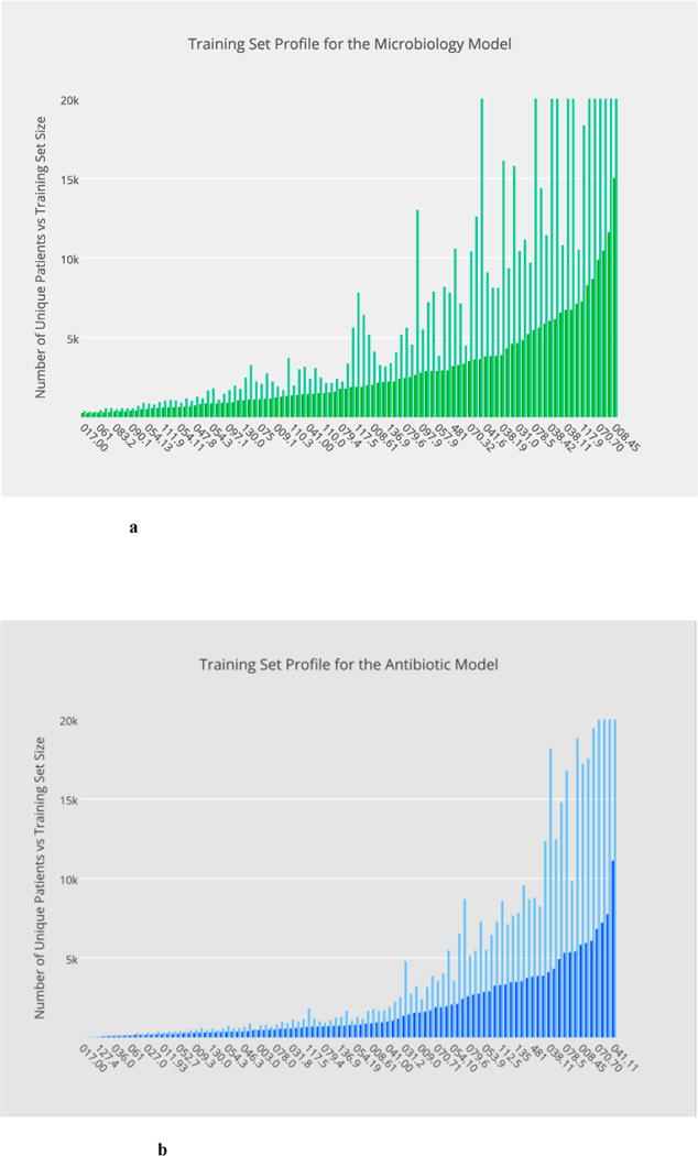
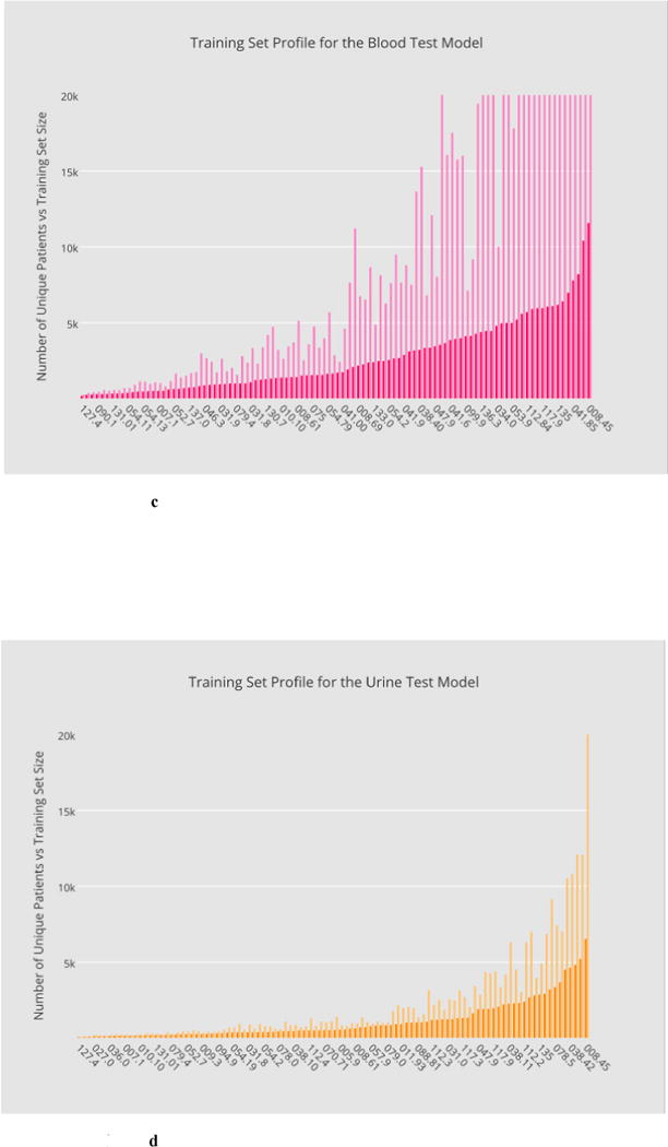
a–d Base-level data profiles of the four phenotypic models in the order of: microbiology, antibiotic, blood test and urine test, respectively, where training set sizes are illustrated in the background in contrast with the number of unique patients in the foreground.

a Distribution of training set sizes for the microbiology model.

b Distribution of training set sizes for the antibiotic model

c Distribution of training set sizes for the blood-test model.

d Distribution of training set sizes for the urine-test model.

3.2 Performance Evaluation of the Learning Hierarchy

The following sections will start off by examining the utility of the feature abstraction in approximating the original ICD-9 labels and subsequently in predicting the annotated sample. In particular, Section 3.2 focuses on the prediction of ICD-9 using only the abstract features. In Section 3.3, we then shift our focus towards predicting an independently annotated sample using statistical models that leverage the tradeoff between abstract features and ICD-9 labels, which now serve as a candidate add-on predictor.

3.2.1 Evaluation of the Base Models Predicting ICD-9

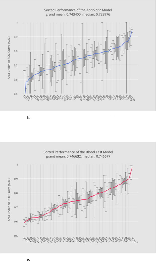
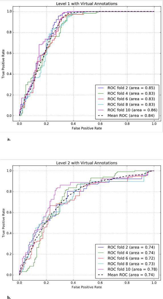
Base model training and evaluation constitute the most computationally expensive part of the bulk learning, which involves computing 400 models, 4 per disease (Section 2.4.1). Fig. 3a through 3d illustrate, in ascending order, the base-level performance in AUC for the bulk learning set represented in ICD-9 codes, each of which is regarded as a different disease for the purpose of this study.

Fig. 3.

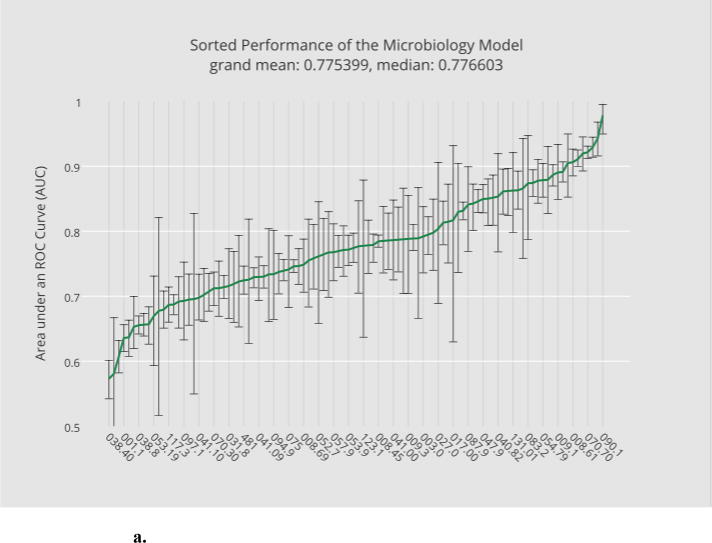
a. Sorted performance of the microbiology model in mean AUCs.

b. Sorted performance of the antibiotic models in their mean AUCs.

c. Sorted performance of the blood-test models in their mean AUCs.

d. Sorted performance of the urine-test models in their mean AUCs.

Each base classifier has different predictive strength due to their varying degrees of clinical relevance to target infections. The microbiology model (Fig. 3a) in general has the highest predictive strength, as expected, with a grand mean of 0.77 (averaged over the scores of all diagnostic codes), which reflects the fact that microorganism tests in general serve as good heuristics for disease predictions. The antibiotic model (Fig. 3b) and the blood-test model (Fig. 3c) have comparable (grand) mean AUCs although the blood-test model exhibits smaller variances. The relatively unstable performance of the antibiotic model can be explained by the fact that not all the selected infectious diseases involve bacterial infections. For instance, enterobiasis (127.4) is a pinworm infection, which, if diagnosed correctly, is often treated by anthelmintics such as mebendazole. The urine-test model has the least predictive strength. Urinalysis is performed typically for cases involving urinary track infections, kidney diseases and sexually transmitted diseases. Venereal disease (099.9) is among the diseases where the urine-test model performs well while candidal esophagitis (112.84) is perhaps less likely to involve urine tests during its diagnosis.

3.2.2 Evaluation of the Level-1 Model Predicting ICD-9

Each member in the bulk learning set has its associated level-1 data obtained from consolidating the base-level predictive results. To examine how effective the level-1 feature representation can differentiate individual disease labels, we constructed 100 local level-1 models and a single global level-1 model: the latter is effectively a combined model of the former (Section 2.4.3). Meanwhile, a separate test set was excluded from all stages of the model training, from the base level to meta-levels, in order to avoid overfitting (see the online supplement, Section M and N, for more details).

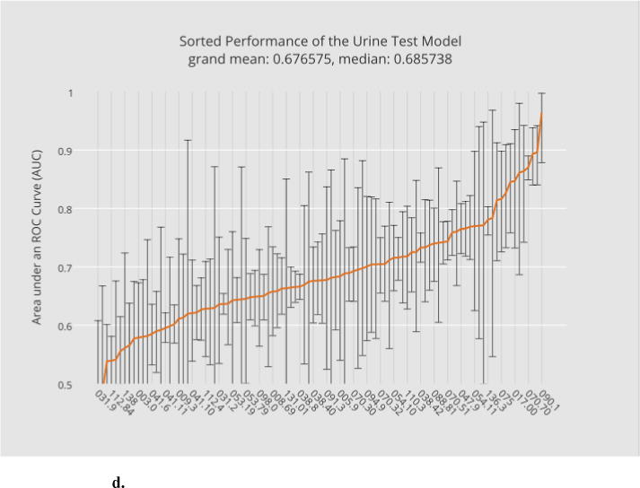
The performance comparison between the level-1 global model and the 100 local level-1 models is given in Fig. 4 under the same task of predicting (binarized) ICD-9 labels of the bulk learning set. In particular, 4a illustrates, in ascending order, the sorted level-1 performance in AUCs for the global model, where the horizontal axis lies the sorted ICD-9 codes and the vertical axis corresponds to their mean AUCs; overlaid at each AUC score is the estimated confidence interval of AUC. The (global) level-1 meta-classifier outperformed the base classifiers on average with the grand mean of the level-1 AUC at 0.895 compared with the largest grand mean of the level-0 AUCs at 0.775 from the microbiology model. This result can be explained by the diversity of the class probability predictions at the base level. Fig. 4b, on the other hand, illustrates the performance for the local level-1 models. The local model exhibited a similar predictive performance with the grand mean AUC at 0.904.

Fig. 4.

a. Performance of the global level-1 model predicting ICD-9s sorted in ascending order of their mean AUCs.

b. The performance of the local level-1 models in ascending order of their mean AUCs.

3.3 Performance Evaluation with the Gold Standard

With sufficient training data, the local model would perform better than the global model. However, using a global model has the advantage of being agnostic to the distribution of sample sizes so that computing statistical models remain feasible even when only few data points are available for individual diseases, a desired property for the upcoming model training and evaluation using the annotated sample. Therefore, we shall only consider the global model henceforth in this section.

In this stage, the abstract features at meta-levels derived earlier from the setup in Section 3.2, i.e. (p, t) at level 1 and p₂ at level 2 respectively, can either be used directly as predictors or serve as part of a larger feature set encompassing other pieces of information. Note that p₂ is simply a probabilistic output of the level-1 classifier predicting ICD-9 (Section 2.4.2).

For experimental purposes, one of the authors (GH) annotated 83 clinical cases indexed by the MRN and dates of the diagnoses. In particular, 54 cases were sampled from the population of positive training examples, corresponding to 54 distinct ICD-9 codes. Similarly, 29 cases were annotated that were sampled from the negative examples associated with 29 distinct ICD-9 codes. For convenience, these two annotation sets are respectively referred to as positive annotations and negative annotations. Note that the polarity, negative or positive, is defined with respect to ICD-9, which is important in further categorizing the annotation types for more detailed performance evaluation in the later sections. The annotated sample was selected at random except that the positive annotation set was made proportionally larger; the sample size was purposefully chosen to be small due to its cost but marginally large enough to train the level-1 model. The data annotation approximately took two weeks to complete even at this scale.

Among the 54 positive annotations, we found 15 instances were falsely classified by ICD-9 whereas all the negative annotations were correctly labeled, giving rise to an overall accuracy at 81.93%. However, there is more subtlety to the calculation of the accuracy. Due to model stacking, the number of annotated clinical cases at the base level is almost never identical to the exact number of training instances derived from these cases. In particular, a patient can have data in more than one base model and within each, there can be more than one training instance due to the possibility of multiple clinical visits at different times. In fact, the 83 annotated cases correspond to 254 training instances at the base level as illustrated in 2^nd and 3^rd columns of Table 4. Nevertheless, the training data, after being transformed into the level-1 representation, will become consistent with the annotated cases in their sizes due to the policy of consolidating data from the base models (Section 2.4.2).

Table 4.

Sizes of the augmented annotation set viewed from the base level where the same clinical case can correspond to multiple training instances.

Annotation Types	Size of Annotated Cases	Size of Authentic Annotations	Size of Virtual Annotations	Total
Type TP (+)	39	119	606	725
Type FP (−)	15	43	160	203
Type TN (−)	29	92	331	423
Type FN (+)	0	0	0	0
All of the above	83	254	1097	1351

3.3.1 The ICD-9 System as a Classifier

The ICD-9, as surrogate labels in the model training, plays a major role in constructing the abstract feature representation and therefore can serve as a good reference for performance comparisons in the upcoming stage of bulk learning. In particular, the ICD-9 system can be regarded as a classifier by considering the diagnostic coding as a form of predictions on disease labels. In the annotated sample where true labels are known, one can categorize an annotation into one of the following four types:

1. Type-TP annotation: Labeled consistently positive by both ICD-9 and the gold standard, this annotated subset herein is referred to as “true positive” annotation, or simply type-TP annotation, since ICD-9 correctly “predicts” positive. Out of the 54 positive annotations, 39 were correctively labeled by ICD-9.

2. Type-FP annotation: Labeled positive by ICD-9 but negative by the gold standard, this annotated subset is referred to as false positive, or type-FP annotation, because ICD-9 falsely predicts positive when the label should have been negative. Out of the 54 positive annotations, 15 were incorrectly labeled by ICD-9.

3. Type-TN annotations: These instances are labeled negative by both ICD-9 and the gold standard and hence they are true negative (TN). All the 29 negative annotations were correctly labeled.

4. Type-FN annotations: Labeled negative by ICD-9 but positive by the gold standard, i.e. false negative, this annotation type does not exist in our data.

Using the annotation type above, we can compute the sensitivity and specificity of “the ICD-9 classifier.” As mentioned earlier, the training set size is not always identical to the number of annotated cases; however, at level-1, they are consistent and therefore, performance calculation is relatively straightforward. In particular, the source of positive examples (by the gold standard) can come from either type-TP or type-FN annotations, giving a total of 39+0=39 instances. Since no false negatives exist (i.e. type-FN annotations), the sensitivity is simply 1. On the other hand, negative examples can be of either type FP or type TN, giving a total of 15+29=44 instances. Therefore, specificity is 0.66, which is obtained by taking the ratio of the size of type TN (29) to that of negative examples (44). An illustration of the annotated sample and its related definitions are given in Table 5, where plus and minus signs denote positive and negative labeling respectively.

Table 5.

A summary of the four annotation types and the performance metrics for the ICD-9 system as a classifier.

Annotation Types	ICD-9	Annotation	Number of Instances	Sensitivity = TP/P = TP/(TP+FN) = 39/(39+0) = 1.00 Specificity = TN/N = TN/(FP+TN) = 29/(15+29) ≈ 0.66 Precision = TP/(TP+FP) = 39/(39+15) ≈ 0.72
TP	+	+	39
FP	+	−	15
TN	−	−	29
FN	−	+	0

3.3.2 The Level-1 and Level-2 Classifiers

Meta-classifiers, upon predicting the annotation set, are evaluated in two different settings: i) using only the abstract features and ii) using an augmented abstract feature set that includes additional predictors such as ICD-9. For the model training and evaluation, we applied repeated 10-fold CV for 30 cycles.

Table 6a shows the performance comparison between the level-1 and level-2 feature representations. The performance of the ICD-9 as a classifier is included as a reference, for which it is possible to simulate an ROC curve and compute its corresponding AUC score by assigning probabilities to its predictive labels under appropriate assumptions. Without a prior knowledge of exactly how clinical data were coded in ICD-9, one could assume, for instance, that the coders were confident in assigning appropriate diagnostic codes to clinical cases; that is, if the ICD-9 were a probabilistic classifier, it would generate a high probability towards 1 to conclude a positive label and by symmetry, a low probability towards 0 to conclude a negative label. This can be simulated by sampling from a negatively skewed distribution between the interval [0.5, 1] and a positively skewed distribution between [0, 0.5). Analogous to the repeated CV, this probability assignment is performed for 30 cycles, resulting in a hypothetical AUC estimate (0.83) for this imaginary ICD-9 classifier.

Table 6a.

Comparison of different meta-classifiers trained with the original annotation set.

Settings	Sensitivity	Specificity	Mean AUC (Repeated 10-fold with 30 cycles)
Level 1 (L1)	583/1170 (0.50)	706/1320 (0.53)	0.520 (0.450 ~ 0.587)
Level 2 (L2)	651/1170 (0.56)	630/1320 (0.48)	0.519 (0.452 ~ 0.585)
L1 + ICD9	921/1170 (0.79)	923/1320 (0.70)	0.79 (0.73 ~ 0.84)
L2 + ICD9	920/1170 (0.79)	896/1320 (0.68)	0.78 (0.71 ~ 0.84)
ICD9	39/39 (1.00)	29/44 (0.66)	0.83 (0.74 ~ 0.92)

Note that the experimental results in Table 6a (and 6b) are specified in fractions followed by their decimal equivalents. In particular, the dominators in all of the metrics are a multiple of 30 as a result of repeating the cross validation 30 times. The level-1 and level-2 features had comparable overall predictive strength with the level-2 model having a slight edge on the sensitivity but not on specificity. However this result is perhaps counterintuitive because the level-2 feature essentially represents a further-smoothed probability with an additional level of model averaging compared to the level 1 and therefore would be expected to be less accurate as a predictor. This is in part due to the small labeled training data (83 instances in total) that led to an easier fit with only one feature at level-2 compared to the level-1 with an 8-D feature set. A remedy to small training set is to augment it with a predefined similarity assumption, as we shall see shortly in Section 3.3.3.

Table 6b.

Comparison by annotation types among different meta-classifier trained with the original annotation set.

Settings	Type TP (39)	Type FP (15)	Type TN (29)	Type FN (0)
Level 1 (L1)	583/1170 (0.50)	200/450 (0.44)	506/870 (0.58)	n/a
Level 2 (L2)	651/1170 (0.56)	218/450 (0.48)	412/870 (0.47)	n/a
L1 + ICD9	921/1170 (0.79)	97/450 (0.22)	826/870 (0.95)	n/a
L2 + ICD9	920/1170 (0.79)	83/450 (0.18)	813/870 (0.93)	n/a
ICD9	39/39 (1.00)	0/15 (0.00)	29/29 (1.00)	n/a

Adding ICD-9 as a feature greatly increases the performance metrics at both levels, as shown in the 3^rd and 4^th row of Table 6a, where the corresponding ICD-9-modulated meta-models are conveniently referred to as L1+ICD9 and L2+ICD9 respectively. In particular, both the sensitivity and specificity shift towards those of the ICD-9 classifier, which indicates that ICD-9 is a stronger predictor compared to abstract features. To understand better the role of the ICD-9 in the prediction of the gold standard, it is helpful to examine the accuracy of predictions in different parts of the labeled data characterized by the four annotations types, which are specified in the header of Table 6b. Since there exist no known annotated data where the ICD-9 committed false negative (i.e. type-FN annotations), its corresponding column does not have experimental results; for the same reason, the accuracy for the type-TP annotation, is exactly identical to the sensitivity since the only source for positive examples are of type TP where the ICD-9 is consistent with the true labels. By contrast, the specificity measure can be derived from the classification accuracies in the region of the type-FP and the type-TN annotations, both nonzero, by simply summing up their numerators and denominators. This algebraic coincidence is due to the fact that sum of the denominators correspond to the total instances of negative examples (by the gold standard), out of which as many as the sum of numerators are correctly classified by the model, equating to the true negative rate. For instance, the specificity of the level-1 model is given by 706/1320 (Table 6a) while its classification accuracy is 200/450 in the type-FP region and 506/870 in the type-TN region, respectively (Table 7b). Since 450 instances were mislabeled by the ICD-9 as positive (when their true labels should have been negative) and 870 instances are indeed negative, there are 450+870=1320 (true) negative instances in total, out of which 200+506=706 were correctly classified by the level-1 model.

Table 7b.

Comparison by annotation types among different meta-classifiers trained by mixing virtual annotations.

Settings	Type TP (39)	Type FP (15)	Type TN (29)	Type FN (0)
Level 1 (L1)	1029/1170 (0.88)	102/450 (0.23)	110/870 (0.13)	n/a
Level 2 (L2)	812/1170 (0.69)	158/450 (0.35)	298/870 (0.34)	n/a
L1 + ICD9	1158/1170 (0.99)	10/450 (0.02)	761/870 (0.87)	n/a
L2 + ICD9	910/1170 (0.78)	104/450 (0.23)	732/870 (0.84)	n/a
Big Logistic	768/1170 (0.66)	276/450 (0.61)	590/870 (0.68)	n/a
Big SVM	784/1170 (0.67)	291/450 (0.65)	571/870 (0.66)	n/a

3.3.3 Introducing Virtual Annotations

Previously, we have seen that the level-2 model produced a counterintuitive empirical result of having comparable performance to the level-1 model, which could have been caused by insufficient labeled data. To potentially increase model performances, a viable solution is to augment the existing training set using virtual annotations. Specifically, for each labeled instance, its corresponding unlabeled data of high affinity are identified through the similarity measure defined in Section 2.4.4, and subsequently, they inherit the same (true) label, assuming that they would have obtained the same labeling due to clinical similarity.

Moreover, to obtain a sample form a wider range of clinical cases, we targeted only those cases with different MRNs. Applying this search strategy allowed us to generate an extra of 1097 labeled instances. In particular, the 4^th column in Table 4 summarizes, by annotation types, the number of virtual annotations, which combined with the original annotation set, leads to an aggregate of 1351 of labeled instances as indicated in last column.

As before, we evaluated the performance of the level-1 and the level-2 models with the absence or presence of ICD-9 as an additional predictor but this time, with the additional labeled data, i.e. virtual annotations. In particular, the process of model training and evaluation remains identical as previous settings except that virtual annotations are excluded from the evaluation. Parallel to the settings in Table 6, Table 7a illustrates the conventional performance metrics while Table 7b further details the performance contribution by annotation types. Moreover, in lieu of the imaginary ICD-9 classifier, we introduce monolithic models as a baseline comparison such as the Big Logistic in Table 7, wherein clinical variables from all the base models, ranging from microbiology to urine test, are combined to form a unified yet relatively large feature set. In particular, ℓ2-regularized logistic classifier is again chosen as the classification algorithm to be consistent with the meta-models based on stacking, although other classifiers such as SVM using various kernels can equally apply. Similar to the level-1 model, we define a single model-consolidated training instance based on the pairing of a unique patient and a class label except that in this case, the best match among all the possible combinations of training instances from across base models, taking into account multiple visits, is resolved by using the shortest time gap as a constraint; that is, the combined instance consists of model-specific constituents with the closest timestamps (e.g. the dates associated with laboratory tests may not coincide exactly with those of medications).

Table 7a.

Comparison of different meta-classifiers trained by mixing virtual annotations.

Settings	Sensitivity	Specificity	Mean AUC (Repeated 10-fold with 30 cycles)
Level 1 (L1)	1029/1170 (0.88)	212/1320 (0.16)	0.59 (0.51 ~ 0.66)
Level 2 (L2)	812/1170 (0.69)	456/1320 (0.35)	0.52 (0.45 ~ 0.60)
L1 + ICD9	1158/1170 (0.99)	771/1320 (0.58)	0.85 (0.80 ~ 0.89)
L2 + ICD9	910/1170 (0.78)	836/1320 (0.63)	0.74 (0.67 ~ 0.82)
Big Logistic	768/1170 (0.66)	866/1320 (0.66)	0.65 (0.59 ~ 0.72)
Big SVM	784/1170 (0.67)	862/1320 (0.65)	0.53 (0.51 ~ 0.56)

With the virtual annotated sample in place, the first noticeable difference is the significant increase of sensitivity in both meta-models (e.g. the sensitivity increased from 0.50 to 0.88 at level 1). However, the specificity dropped for both models, where the drop is more noticeable within the type-TN region. By introducing ICD-9 as a predictor, both sensitivity and specificity were increased significantly as shown in Table 7b. A closer look at the performance by annotation types, however, suggests that only the type-TN region of data contributed to the improvement in specificity, the type-FP component of which was in fact deteriorated. The L1+ICD9 model, for instance, improved its type-TN accuracy from 0.13 to 0.87 whereas its type-FP accuracy dropped from 0.23 to 0.02. This performance profile is substantially closer to the ICD-9 classifier (shown in the last row of Table 6), suggesting the dominance of the ICD-9 as a predictor. The abstract features, however, play the role of modulating the ICD-9 signal (and vise versa), which allows for some correct labeling to occur in the type-FP region. In particular, the L2+ICD9 model has a better type-FP accuracy than its level-1 counterpart due to a higher level of model averaging. By contrast, the L1+ICD9 model has a better overall performance including sensitivity, AUC and the accuracy in most annotated sample except for those in the type-FP region.

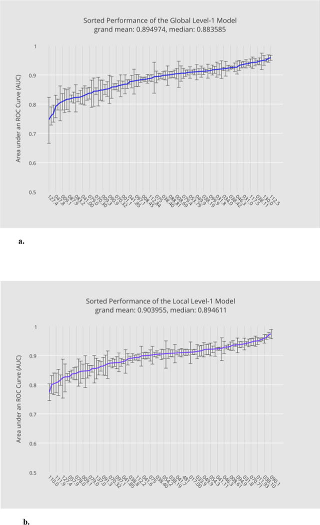
The monolithic model does not generally have a performance-wise advantage due to its relatively smaller ratio between the training sample size³ and the feature dimension⁴, which inevitably leads to model overfitting and large variances in AUC scores within each cross validation cycle (albeit not as prominent after averaging over 30 CV-cycles). The monolithic model, however, had a relatively better accuracy in the type FP region. Similar results were observed in the case of Big SVM⁵ (Table 7). Last but not least, Fig. 5a and Fig. 5b compare the ROC curves of the ICD-9-modulated models at level 1 and level 2 respectively.

Fig. 5.

a. The performance of the ICD-9-modulated level-1 model trained with virtual annotations.

b. The performance of the ICD-9-modulated level-2 model trained with virtual annotations.

4. Discussion

From the empirical results, we have demonstrated the possibility of using a small annotation set for achieving statistical model training and evaluation by constructing abstract feature representations on top of the phenotypic models of the bulk learning set. Feature abstraction allows for a reduction of feature space on which statistical models are built, leading to a reduced demand for labeled data.

The process of consolidating base models to formulate the level-1 abstraction, in particular, presents the first opportunity in the reduction of the required annotated data. A comparison between the level-0 and the level-1 performances in Fig. 3 and Fig. 4 suggests that an appropriate combination of the base ensembles leads to aggregate models, including the global and local level-1 models, that exhibit relatively superior classification performance on average.

In particular, each local level-1 model is effectively an ensemble of disease-specific base models. A further reduction of required labeled data can be achieved through the ensemble of the clinical cases across different diseases, leading to a global level-1 model. In this case, as long as the size of the combined labeled data is sufficient for the level-1 feature representation, learning a predictive model remains feasible and potentially without much loss of performance, as evidenced by contrasting Fig. 4a and 4b, although we believe this property would also depend on the disease composition of the bulk learning set. Nevertheless, the global model becomes a more feasible option when the majority of the diseases have very limited data points – the case for the annotated sample in practice. An intermediate alternative to the global model, if a larger annotated sample were available, would be to compute clustered disease models based on the aggregation of similar diseases (instead of the entire annotated sample) using diagnostic codes as heuristics.

The mechanism of the feature abstraction can influence the classification performance as we have seen in the experimental settings. With sufficient training data, the abstract feature representation at a lower level in general has better predictive strength since in essence, the higher the level goes, the more model averaging is involved.

Including ICD-9 as an extra predictor increased the model performance further due to the fact that the ICD-9 itself is a good approximation to the gold standard with disagreements only in the type-FP region, which constitutes a relatively small portion of the annotated sample. Using abstract features as a channel to modulate the ICD-9 signal, however, opens the possibility for the models at meta-levels to shift towards closing the gap between the ICD-9 and the gold standard albeit not prominent in the current experimental settings, for which the main challenge lies in the capacity to predict type FP (where ICD-9 committed errors).

We have seen various performance tradeoffs in attempting to boost the predictive accuracy in the type-FP region by mixing the ICD-9 and abstract features, and incorporating virtual annotations generated from the original annotation set. The interested reader is encouraged to refer to the supplementary document (Section R and S) for additional experimental settings and analyses. We believe that a further fine turning in the semi-supervised learning approach by balancing the positive and negative annotated sample (e.g. generating a larger type-FP sample) would further increase the overall predictive performance. Alternatively, one could incorporate higher-order abstract features to induce a complex, non-linear decision boundary, provided that the sample size of the labeled data is sufficiently large (e.g. using virtual annotations). Applying the same bulk learning method using multiple surrogate labels in parallel is also a promising solution (see Section L in the supplement).

As noted in Section 3, monolithic models that combine feature sets from across phenotypic models do not generally have a performance advantage mainly due to a sizably smaller ratio between the sample size (n) and the feature dimension (p), especially when considering the annotated sample as a limited resource. A monolithic feature set tends to exhibit unnecessary redundancies, being less compact due to missing values associated with an entire phenotypic model (e.g. lack of specific lab tests as discussed in Section 2.4.2). While we have not comprehensively demonstrated superiority of the stacked model over alternatives for overall predictive performance, however, we wish to motivate an alternative patient representation, as discussed in Section 2.2.2, that leverages medical ontology by using it as a conduit for grouping conceptually related variables such that smaller models can be established leading to a higher modularity.

Ontology-based feature engineering integrates seamlessly with the model stacking methodology. Nonetheless, this vantage point is only achieved when the assumption holds that the healthcare institution maintains a consistent medical coding between the medical ontology and the data warehouse. OHDSI [51], for instance, is a collaborative effort that contributes to unified concept mappings across different coding standards. On the other hand, although we have used infectious diseases as an example domain for which ontological feature selection works well, other disease classes such as cardiac and neurological diseases where dedicated tests and treatments are available that can be modularized into conceptual categories could also benefit from this method. Patients with autoimmune diseases tend to have high susceptibility to infections, which potentially correspond to a common treatment pathway where the four example phenotypic models given in Section 2.3 could become relevant.

So far, we have only focused on a three-tier stacking architecture for illustrative purposes; however, there is no restriction in the allowable levels of abstraction by decomposing a phenotypic model further into smaller constituent models. For instance, we have seen in Fig. 3b that the antibiotic model has relatively low and unstable performance (with high variances) in certain diseases that do not normally involve antibiotic prescriptions as a treatment plan. A more comprehensive phenotypic unit for medicinal treatments would be by itself a two-tier model where the lower level, in addition to antibiotics, comprises the other pathogen-specific models, such as anthelmintics and antivirals; subsequently, these treatment models are combined at the meta-level through the tradeoff by weights, best model selection, among other model combing strategies. Furthermore, there is much flexibility in the design of the stacking architecture, including cascading meta-levels, partial phenotypic models with various feature subsets from a single phenotypic group, and dynamic integration of phenotypic ensembles to account for concept drifts (e.g. pathogen sensitivity shifting over time due to antibiotic resistance [41]), among many others.

To the best of our knowledge, this is one of the very few, if not the first, studies that attempt to achieve batch-phenotyping over multiple diseases using only a sparse annotation set curated from EHR data while other work tackles diverse disease phenotyping primarily from the angles of automated feature extraction [1,21,22] and knowledge engineering [22,42,43]. Methodologically speaking, however, learning phenotypes from noisy labels has two ongoing research directions that are interrelated, i.e. modeling phenotypes from anchor variables [44,45] and silver-standard training data [46]. We also note that from the perspective of learning shared representations of diseases (such as the abstraction feature representation in this study), contemporary phenotyping effort has led to a growing body of work that learns phenotypes from population-scale clinical data using the methodology of representation learning [47,48] including i) spectral learning such as non-negative tensor factorization [5], ii) probabilistic mixture models [8], and additionally, when temporal phenotypic patterns are considered, iii) unsupervised feature learning using autoencoders [32] and latent medical concepts [49], etc., and iv) deep learning [6].

5. Conclusions and Future Work

The essence of the bulk learning is to phenotype multiple diseases of the same class (e.g. a set of infectious diseases) simultaneously, which renders the possibility of representing the underlying clinical cases, as a whole, in units of shared phenotypic components expressing unique clinical aspects in the diagnoses and treatments common to at least a subset of the diseases. Using the phenotypic components as building blocks for constructing ensembles of classifiers facilitates the unraveling of shared clinical patterns, encoded within the tradeoff of each ensemble driven by stacked generalization that serves as the basis for defining feature abstractions. Subsequently, the dimensionality of the training data is reduced from the large feature space, comprising vast EHR variables, down to a relatively compact abstract feature space. In essence, the layer of feature abstraction is what leads to the minimizing of required training data for establishing predictive models, thereby alleviating the data annotation effort in phenotyping tasks.

Using ICD-9 as surrogacy enables the training of component phenotypic models without annotated data. For future work, however, it is worth investigating other types of surrogate labels beyond diagnostic codes such as the keywords extracted from clinical notes and their derived constructs such as anchors [44]. Furthermore, we have only demonstrated a three-level stacking architecture as a compact example to illustrate the potential of simultaneous disease phenotying. In general, it is possible to design a deeper stacking hierarchy where each tier contains multiple fine-grained component phenotypic models (e.g. pathogen-specific treatment models) towards an even finer control of the feature space dimension and a better tradeoff in sample complexity required to find good classifiers.

Identifying representative clinical cases as the gold standard is yet another important step towards improving the model performance in that the derived abstract features, under such setting, could serve as a better compact representation of the bulk learning set. In this study, the annotation candidates were selected at random within each disease and consequently might not represent the population very well. This would in turn also influence the quality of virtual annotation set. In order to leverage the semi-supervised learning approach, we believe that active learning [50] on annotation candidates (i.e. an interactive selection of informative unlabeled instances for annotations) would promote a higher generalizability of the virtual annotations, which drives up the classification performance of the bulk learning system with potentially more well-defined decision boundaries between any two annotation types.

References

- 1.Yu S, Liao KP, Shaw SY, et al. Toward high-throughput phenotyping: unbiased automated feature extraction and selection from knowledge sources. J Am Med Informatics Assoc. 2015:993–1000. doi: 10.1093/jamia/ocv034. [DOI] [PMC free article] [PubMed] [Google Scholar]
- 2.Delude CM. Deep phenotyping: The details of disease. Nature. 2015;527:S14–S15. doi: 10.1038/527S14a. [DOI] [PubMed] [Google Scholar]
- 3.Robinson PN. Deep phenotyping for precision medicine. Hum Mutat. 2012;33:777–780. doi: 10.1002/humu.22080. [DOI] [PubMed] [Google Scholar]
- 4.Newton KM, Peissig PL, Denny JC, et al. Validation of electronic medical record-based phenotyping algorithms: results and lessons learned from the eMERGE network. J Am Med Informatics Assoc. 2013;20:e147–e154. doi: 10.1136/amiajnl-2012-000896. [DOI] [PMC free article] [PubMed] [Google Scholar]
- 5.Ho J, Ghosh J, Sun J. Marble : High-throughput Phenotyping from Electronic Health Records via Sparse Nonnegative Tensor Factorization. Proc 20th ACM SIGKDD Int Conf Knowl Discov Data Min - KDD ’14. 2014:115–124. doi: 10.1145/2623330.2623658. [DOI] [Google Scholar]
- 6.Che Z, Kale D, Li W, Bahadori MT, Liu Y. Deep Computational Phenotyping; Proc. 21th ACM SIGKDD Int. Conf. Knowl. Discov. Data Min. - KDD ’15; New York, USA. New York: ACM Press; 2015. pp. 507–516. [DOI] [Google Scholar]
- 7.Chen Y, Carroll RJ, Xu H, et al. Applying active learning to high-throughput phenotyping algorithms for electronic health records data. J Am Med Informatics Assoc. 2013;20:1–7. doi: 10.1136/amiajnl-2013-001945. [DOI] [PMC free article] [PubMed] [Google Scholar]
- 8.Pivovarov R, Perotte AJ, Grave E, Angiolillo J, Wiggins CH, Elhadad N. Learning probabilistic phenotypes from heterogeneous EHR data. J Biomed Inform. 2015;58:156–165. doi: 10.1016/j.jbi.2015.10.001. [DOI] [PMC free article] [PubMed] [Google Scholar]
- 9.Wilcox AB. The Role of Domain Knowledge in Automating Medical Text Report Classification. J Am Med Informatics Assoc. 2003;10:330–338. doi: 10.1197/jamia.M1157. [DOI] [PMC free article] [PubMed] [Google Scholar]
- 10.Wolpert DH. Stacked generalization. Neural Networks. 1992;5:241–259. doi: 10.1016/S0893-6080(05)80023-1. [DOI] [Google Scholar]
- 11.Ting KM, Witten IH. Issues in stacked generalization. J Artif Intell Res. 1999;10:271–289. doi: 10.1613/jair.594. [DOI] [Google Scholar]
- 12.Jin Chen J, Cheng Wang C, Runsheng Wang R. Using Stacked Generalization to Combine SVMs in Magnitude and Shape Feature Spaces for Classification of Hyperspectral Data. IEEE Trans Geosci Remote Sens. 2009;47:2193–2205. doi: 10.1109/TGRS.2008.2010491. [DOI] [Google Scholar]
- 13.Wang SQ, Yang J, Chou KC. Using stacked generalization to predict membrane protein types based on pseudo-amino acid composition. J Theor Biol. 2006;242:941–946. doi: 10.1016/j.jtbi.2006.05.006. [DOI] [PubMed] [Google Scholar]
- 14.O’Malley KJ, Cook KF, Ashton CM, et al. Measuring diagnoses: ICD code accuracy. Health Serv Res. 2005;40:1620–39. doi: 10.1111/j.1475-6773.2005.00444.x. [DOI] [PMC free article] [PubMed] [Google Scholar]
- 15.Farzandipour M, Sheikhtaheri A, Sadoughi F. Effective factors on accuracy of principal diagnosis coding based on International Classification of Diseases, the 10th revision (ICD-10) Int J Inf Manage. 2010;30:78–84. doi: 10.1016/j.ijinfomgt.2009.07.002. [DOI] [Google Scholar]
- 16.Belkin M, Niyogi P. Laplacian Eigenmaps for Dimensionality Reduction and Data Representation. Neural Comput. 2003;15:1373–1396. doi: 10.1162/089976603321780317. [DOI] [Google Scholar]
- 17.Mao KZ. Orthogonal Forward Selection and Backward Elimination Algorithms for Feature Subset Selection. IEEE Trans Syst Man Cybern Part B. 2004;34:629–634. doi: 10.1109/TSMCB.2002.804363. [DOI] [PubMed] [Google Scholar]
- 18.Kohavi R, John GH. Wrappers for feature subset selection. Artif Intell. 1997;97:273–324. doi: 10.1016/S0004-3702(97)00043-X. [DOI] [Google Scholar]
- 19.Zou H, Hastie T. Regularization and variable selection via the elastic-net. J R Stat Soc. 2005;67:301–320. doi: 10.1111/j.1467-9868.2005.00503.x. [DOI] [Google Scholar]
- 20.Yuan M, Lin Y. Model selection and estimation in regression with grouped variables. J R Stat Soc Ser B Stat Methodol. 2006;68:49–67. doi: 10.1111/j.1467-9868.2005.00532.x. [DOI] [Google Scholar]
- 21.Shivade C, Raghavan P, Lai AM, et al. A review of approaches to identifying patient phenotype cohorts using electronic health records. J Am Med Inform Assoc. 2013;21:221–30. doi: 10.1136/amiajnl-2013-001935. [DOI] [PMC free article] [PubMed] [Google Scholar]
- 22.Lyalina S, Percha B, Shah NH, et al. Identifying phenotypic signatures of neuropsychiatric disorders from electronic medical records. J Am Med Inform Assoc. 2013;20:e297–305. doi: 10.1136/amiajnl-2013-001933. [DOI] [PMC free article] [PubMed] [Google Scholar]
- 23.Li LL, Cheng WYW, Dudley JT, et al. Identification of type 2 diabetes subgroups through topological analysis of patient similarity. Sci Transl Med. 2015;7:1–16. doi: 10.1126/scitranslmed.aaa9364. [DOI] [PMC free article] [PubMed] [Google Scholar]
- 24.Lowy FD. Staphylococcus aureus Infections. N Engl J Med. 1998;339:520–532. doi: 10.1056/NEJM199808203390806. [DOI] [PubMed] [Google Scholar]
- 25.Baorto D, Cimino J. Medical Entities Dictionary. 2016 http://med.dmi.columbia.edu/ (accessed 10.05.2016)
- 26.Cimino JJ, Clayton PD, Hripcsak G, Johnson SB. Knowledge-based approaches to the maintenance of a large controlled medical terminology. J Am Med Inform Assoc. 1994;1:35–50. doi: 10.1136/jamia.1994.95236135. [DOI] [PMC free article] [PubMed] [Google Scholar]
- 27.Bodenreider O. The Unified Medical Language System (UMLS): integrating biomedical terminology. Nucleic Acids Res. 2004;32:267D–270. doi: 10.1093/nar/gkh061. [DOI] [PMC free article] [PubMed] [Google Scholar]
- 28.Bach F. Bolasso: model consistent Lasso estimation through the bootstrap. Proc 25th Int Conf Mach Learn. 2008:33–40. doi: 10.1145/1390156.1390161. [DOI] [Google Scholar]
- 29.Rokach L. Ensemble-based classifiers. Artif Intell Rev. 2010;33:1–39. doi: 10.1007/s10462-009-9124-7. [DOI] [Google Scholar]
- 30.Choraś M, Bhanu B, Liu Z, et al. Encycl Biometrics. Springer US; Boston, MA: 2009. Ensemble Learning; pp. 270–273. [DOI] [Google Scholar]
- 31.Kuncheva LI. DERA/IEE Work Intell Sens Process. IEE; 2001. Ten measures of diversity in classifier ensembles: limits for two classifiers; pp. 10–10. [DOI] [Google Scholar]
- 32.Lasko TA, Denny JC, Levy MA. Computational Phenotype Discovery Using Unsupervised Feature Learning over Noisy, Sparse, and Irregular Clinical Data. PLoS One. 2013;8:e66341. doi: 10.1371/journal.pone.0066341. [DOI] [PMC free article] [PubMed] [Google Scholar]
- 33.Gama J, Brazdil P. Cascade Generalization. Mach Learn. 2000;41:315–343. doi: 10.1023/A:1007652114878. [DOI] [Google Scholar]
- 34.Zhao H, Ram S. Constrained cascade generalization of decision trees. IEEE Trans Knowl Data Eng. 2004;16:727–739. doi: 10.1109/TKDE.2004.3. [DOI] [Google Scholar]
- 35.Džeroski S, Ženko B. Is Combining Classifiers with Stacking Better than Selecting the Best One? Mach Learn. 2004;54:255–273. doi: 10.1023/B:MACH.0000015881.36452.6e. [DOI] [Google Scholar]
- 36.Woźniak M, Graña M. A survey of multiple classifier systems as hybrid systems. Inf Fusion. 2014;16:3–17. doi: 10.1016/j.inffus.2013.04.006. [DOI] [Google Scholar]
- 37.Niculescu-Mizil A, Caruana R. Predicting good probabilities with supervised learning; Proc. 22nd Int. Conf. Mach. Learn. ICML 05; 2005. pp. 625–632. [DOI] [Google Scholar]
- 38.Zhou ZH, Zhan DC, Yang Q. Semi-Supervised Learning with Very Few Labeled Training Examples. Artif Intell. 2005;22:675–680. [Google Scholar]
- 39.Wu J, Diao YB, Li ML, Fang YP, Ma DC. A semi-supervised learning based method: Laplacian support vector machine used in diabetes disease diagnosis. Interdiscip Sci Comput Life Sci. 2009;1:151–155. doi: 10.1007/s12539-009-0016-2. [DOI] [PubMed] [Google Scholar]
- 40.Dhillon IS, Fan J, Guan Y. Efficient clustering of very large document collections. Data Min Sci Eng Appl. 2001:357–381. [Google Scholar]
- 41.Tsymbal A, Pechenizkiy M, Cunningham P, Puuronen S. Dynamic integration of classifiers for handling concept drift. Inf Fusion. 2008;9:56–68. doi: 10.1016/j.inffus.2006.11.002. [DOI] [Google Scholar]
- 42.Pathak J, Wang J, Brandt S, et al. Mapping clinical phenotype data elements to standardized metadata repositories and controlled terminologies: the eMERGE Network experience. J Am Med Inform Assoc. 2011;18:376–86. doi: 10.1136/amiajnl-2010-000061. [DOI] [PMC free article] [PubMed] [Google Scholar]
- 43.Donnelly K. SNOMED-CT: The advanced terminology and coding system for eHealth. Stud Health Technol Inform. 2006;121:279–90. [PubMed] [Google Scholar]
- 44.Halpern Y, Choi Y, Horng S, Sontag D. Using Anchors to Estimate Clinical State without Labeled Data. AMIA Annu Symp Proc. 2014;2014:606–15. [PMC free article] [PubMed] [Google Scholar]
- 45.Halpern Y, Horng S, Choi Y, Sontag D. Electronic medical record phenotyping using the anchor and learn framework. J Am Med Informatics Assoc. 2016;23:731–740. doi: 10.1093/jamia/ocw011. [DOI] [PMC free article] [PubMed] [Google Scholar]
- 46.Agarwal V, Podchiyska T, Shah NH, et al. Learning statistical models of phenotypes using noisy labeled training data. J Am Med Informatics Assoc. 2016:ocw028. doi: 10.1093/jamia/ocw028. [DOI] [PMC free article] [PubMed] [Google Scholar]
- 47.Bengio Y, Courville A, Vincent P. Representation Learning: A Review and New Perspectives. IEEE Trans Pattern Anal Mach Intell. 2013;35:1798–1828. doi: 10.1109/TPAMI.2013.50. [DOI] [PubMed] [Google Scholar]
- 48.Liao S, Gao Y, Oto A, Shen D. Representation Learning: A Unified Deep Learning Framework for Automatic Prostate MR Segmentation, in. Springer Berlin Heidelberg. 2013:254–261. doi: 10.1007/978-3-642-40763-5_32. [DOI] [PMC free article] [PubMed] [Google Scholar]
- 49.Zhou J, Wang F, Hu J, Ye J. From Micro to Macro: Data Driven Phenotyping by Densification of Longitudinal Electronic Medical Records; Proc. 20th ACM SIGKDD Int. Conf. Knowl. Discov. Data Min; 2014. pp. 135–144. [DOI] [Google Scholar]
- 50.Settles B. From Theories to Queries: Active Learning in Practice. Proc Work Act Learn Exp Des. 2011;16:1–18. [Google Scholar]
- 51.Hripcsak G, Ryan PB, Duke JD, et al. Observational Health Data Sciences and Informatics (OHDSI): Opportunities for Observational Researchers. Stud Health Technol Inform. 2015:574–578. doi: 10.3233/978-1-61499-564-7-574. [DOI] [PMC free article] [PubMed] [Google Scholar]
Associated Data
This section collects any data citations, data availability statements, or supplementary materials included in this article.