Semi‐automated pulmonary nodule interval segmentation using the NLST data

Abstract

Purpose

To study the variability in volume change estimates of pulmonary nodules due to segmentation approaches used across several algorithms and to evaluate these effects on the ability to predict nodule malignancy.

Methods

We obtained 100 patient image datasets from the National Lung Screening Trial (NLST) that had a nodule detected on each of two consecutive low dose computed tomography (LDCT) scans, with an equal proportion of malignant and benign cases (50 malignant, 50 benign). Information about the nodule location for the cases was provided by a screen capture with a bounding box and its axial location was indicated. Five participating quantitative imaging network (QIN) institutions performed nodule segmentation using their preferred semi‐automated algorithms with no manual correction; teams were allowed to provide additional manually corrected segmentations (analyzed separately). The teams were asked to provide segmentation masks for each nodule at both time points. From these masks, the volume was estimated for the nodule at each time point; the change in volume (absolute and percent change) across time points was estimated as well. We used the concordance correlation coefficient (CCC) to compare the similarity of computed nodule volumes (absolute and percent change) across algorithms. We used Logistic regression model on the change in volume (absolute change and percent change) of the nodules to predict the malignancy status, the area under the receiver operating characteristic curve (AUROC) and confidence intervals were reported. Because the size of nodules was expected to have a substantial effect on segmentation variability, analysis of change in volumes was stratified by lesion size, where lesions were grouped into those with a longest diameter of <8 mm and those with longest diameter ≥ 8 mm.

Results

We find that segmentation of the nodules shows substantial variability across algorithms, with the CCC ranging from 0.56 to 0.95 for change in volume (percent change in volume range was [0.15 to 0.86]) across the nodules. When examining nodules based on their longest diameter, we find the CCC had higher values for large nodules with a range of [0.54 to 0.93] among the algorithms, while percent change in volume was [0.3 to 0.95]. Compared to that of smaller nodules which had a range of [−0.0038 to 0.69] and percent change in volume was [−0.039 to 0.92]. The malignancy prediction results showed fairly consistent results across the institutions, the AUC using change in volume ranged from 0.65 to 0.89 (Percent change in volume was 0.64 to 0.86) for entire nodule range. Prediction improves for large nodule range (≥ 8 mm) with AUC range 0.75 to 0.90 (percent change in volume was 0.74 to 0.92). Compared to smaller nodule range (<8 mm) with AUC range 0.57 to 0.78 (percent change in volume was 0.59 to 0.77).

Conclusions

We find there is a fairly high concordance in the size measurements for larger nodules (≥8 mm) than the lower sizes (<8 mm) across algorithms. We find the change in nodule volume (absolute and percent change) were consistent predictors of malignancy across institutions, despite using different segmentation algorithms. Using volume change estimates without corrections shows slightly lower predictability (for two teams).

1. Introduction

Lung cancer is the leading cause of cancer deaths in the United States.¹ However, early detection with low dose CT (LDCT) was shown to reduce lung cancer specific mortality by the National Lung screening Trial (NLST).² These effects are also being investigated in another ongoing international effort, the Dutch‐Belgian randomized lung cancer (NELSON) Trial.³ Specifically, the results of NLST study showed a 20% relative reduction in lung cancer related mortality compared with screening using chest radiography.⁴ This resulted the Center for Medicare and Medicaid Services (CMS) to recommend the use of low dose CT for lung cancer screening.⁵ Other organizations, such as the American College of Radiology (ACR) followed suite to provide resources to those centers wishing to perform imaging studies.⁶ Though the use of LDCT led to the detection of more nodules compared to chest radiographs, and which may aid early diagnosis of lung cancer, but the trial also showed higher incidence of false positives.⁷

Identification of a nodule on an LDCT screening exam can represent a positive image finding based on the size of the nodule, which may then be followed up by a secondary confirmation procedure to determine malignancy of the nodule. To date clinically, screen detected positivity is based on size of the nodule; for example, in the ACR Lung CT Screening Reporting and Data System (Lung‐RADS), solid nodules with a diameter < 6 mm are considered to be negative and risk cannot be ascertained or Lung‐RADS category 1.⁸ Estimating the size of these lung nodules during the screening intervals is an important clinical factor in the determination of patient's follow‐up procedure. Recent studies have shown the utility of tumor volume as a better estimator of tumor growth ⁹ and it has shown to be more useful than the conventional unidimensional (diameter) measurements. It has been suggested that doubling time based on nodule volume may also be used as a predictive measure of malignancy.¹⁰ Recently, doubling time was used to suggest a risk stratification for screening patients.¹¹

It is essential to accurately measure the nodule size, which can have direct clinical implications, including the selection of treatment procedures. There have been many studies that focused on nodule size estimation in the past,^{12, 13} which investigated the bias and variability issues in the size measurements.

In an effort to quantitate variability among different segmentation algorithms to delineate the nodules identified over two screening intervals, we proposed a multi‐institutional study with members of the quantitative imaging network (QIN) to estimate variability in size/volume estimation using their preferred methods using current advancements in segmentation methods. We hypothesize that any fixed biases that may exist in single time point segmentations for a method would be offset with a subsequent segmentation and computing change estimates, in size/volume for a nodule.

In this study, we used the data from the National Lung Screening Trial (NLST) and assembled a cohort of patients with nodules that were identified across screening time points.^{7, 8} We had five participating sites (MCC/USF: Moffitt Cancer Center/University of South Florida, CUMC: Columbia University Medical Center, UMICH: University of Michigan, DFCC: Dana Farber Cancer Center, UCLA: University of California at Los Angeles) that used different segmentation algorithms for performing the nodule delineation, and two additional sites participated with their analytics expertise (SU:Stanford University, MGH:Massachusetts General Hospital). The teams were allowed to use local expertise and preferred segmentation procedures and report back the segmentation masks.

In our analysis, we evaluated similarity in the segmentations by computing the concordance correlation on the volume and change in volume estimations across the five participants. We then built independent prediction model using logistic regression to relate volume change and percent volume change estimates obtained from the segmentation masks to the nodules malignancy status. We then compared ability of each site's volume estimates (and change in volume) to predict the malignancy using Area Under the receiver operating characteristic Curve or AUC. We further divided the cohort based on nodule size ranges (baseline size ≥ 8 mm, < 8 mm) and repeated the predictive analysis based on the nodule volumes and change in volumes across time. Our study work flow is shown in Fig. 1 with an example pulmonary nodule across time points.

Figure 1.

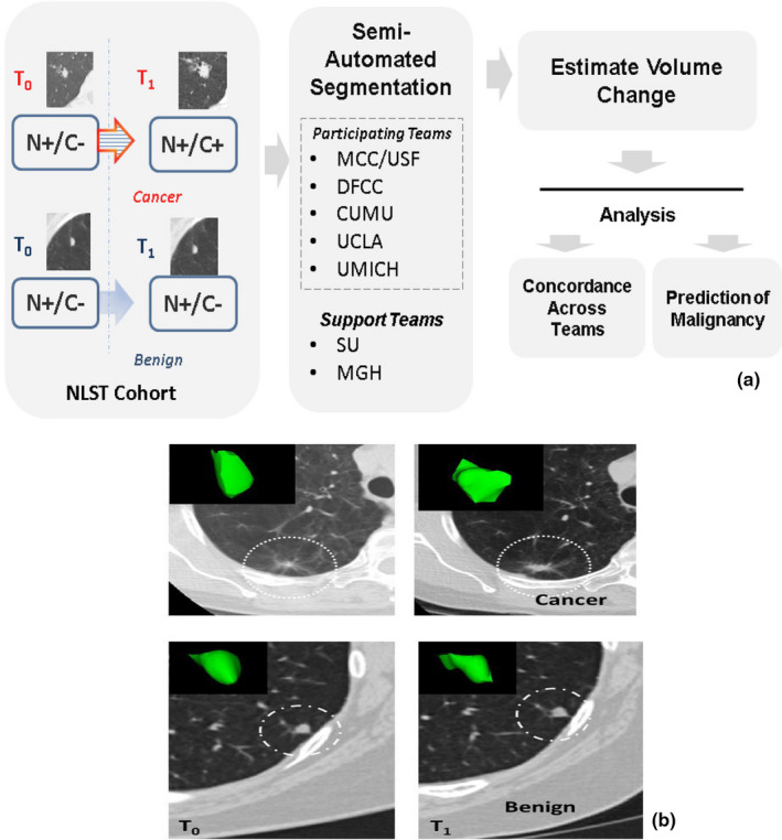
Describes the multi‐institutional study, (a) Process work flow of the study and (b) Representative patient scans (2D, center slice) at different screening intervals for nodules diagnosed to be malignant and benign (non‐cancerous) at follow‐up scan. The teams are: Moffitt Cancer Center/University of South Florida (MCC/USF), Dana Faber Cancer Center (DFCC), Columbia University Medical Center (CUMU), and University of California at Los Angeles Medical Center (UCLA), University of Michigan Medical Center (UMICH), Stanford University (SU), and Massachusetts General Hospital (MGH). [Color figure can be viewed at wileyonlinelibrary.com]

2. Material and methods

2.A. NLST study design and data access

The National Lung Screening Trial was the largest clinical trial in the U.S with an enrollment of 53,439 participants, of which half the population was randomly assigned to LDCT study arm and the other half was randomized to chest radiography. The participants were between 55 to 74 yr of age and were high risk individuals that were either current or former smokers with a 30+ pack‐year smoking history (former smokers had to have quit smoking in the last 15 yr). These participants were enrolled across 33 U.S institutions and were screened at baseline (T0) and annually for two additional years (T1 and T2). For those participants randomized to the CT arm of the study, a low dose lung cancer screening CT was performed according to a specified imaging protocol.¹⁴ The study defined a positive screen as a non‐calcified nodule (NCN) ≥ 4 mm in diameter. The NLST radiologist reported the location, composition (solid, part‐solid, ground‐glass), margin and other observed characteristics for all identified nodules.

The patient records from the NLST were obtained from the CDAS (Cancer Data Access System) and the imaging data through the TCIA (The Cancer Imaging Archive), after starting a study protocol at the Moffitt Cancer Center. All the participants of the study were added to the protocol and the participants of the study executed a data transfer agreement (DTA) at their respective institutions with the National Cancer Institute (NCI). The study was approved by the University of South Florida's Institutional Review Board (IRB) to lead the investigation at Moffitt Cancer Center and each of the participating institutions obtained de‐identified patient records, which waives the need for individual institutional review.

2.2. Interval challenge study cohort

We identified 100 subjects with nodules identified on CT scans at baseline and follow up, making a total of 200 CT image datasets. Each selected case had at least one nodule that met the NLST protocol guidelines (≥ 4 mm).² In our study, we selected equal number of cases that were confirmed to be cancer and those confirmed to be non‐cancerous or nodule‐positive benign (50 cancer subjects and 50 benign subjects). Our resident radiologists verified the NLST provided information for the entire cohort used for the study. The cases included in the study were followed across available screening intervals and were verified the location on the scan. We selected one nodule per patient that had largest measured diameter following the NLST study criteria (≥ 4 mm). For the benign cases, we used the baseline and the follow up scans to identify stable positive nodules in the cohort. The nodule size distribution is shown in Table 1.

Table 1.

Pulmonary nodule characteristics for the patient cohort across the screening time points

Categories (longest diametera)	Total		Cancerb		Benignb
	Baseline (T0)	Follow‐up (T1)	Baseline (T0)	Follow‐up (T1)	Baseline (T0)	Follow‐up (T1)
All Nodules	100	100	50	50	50	50
< 8 mm	50	44	18	9	32	35
≥ 8 mm	50	56	32	41	18	15

^aBased on Team 3A's size estimates.

^bBased on diagnosis at follow‐up time point (T1).

The identified nodule in the study cohort was provided to the participants with an axial slice location (need not be the center) and an identifying box over the nodule. The clinical diagnosis and exact coordinates including nodule centers were not disclosed. This was done to avoid potential bias in the segmentation procedures between participants. The teams were asked to segment the nodules in each of the 100 cases using their preferred segmentation approach. We allowed fully automated or semi‐automated procedures for this effort, where no restriction was placed on the seeding information for the teams respective algorithms. We did not allow complete manual segmentation procedure in this study. Each participating site agreed to submit at least one set of segmentation results without any manual editing of the resulting nodule contours. Sites were provided an option to submit additional results where editing of the nodule boundaries was allowed and these were analyzed separately. Figure 1(b) shows two sample patients with diagnosed cancer and benign nodules at two consecutive time intervals.

2.3. Multi‐institutional collaborative study

All the participants were part of the quantitative imaging network (QIN) funded institutions. Because of the diversity of available tools and approaches, the study group collaboratively reached agreement on several key technical details and procedures to facilitate the study's goals. These included agreeing on image data format (DICOM), case and nodule information provided to participants (as described above), segmentation procedures allowed (as described above), annotation formats allowed (DICOM‐SEG and NIFTI) as well as an analysis study document describing the study analyses to be performed. Although there are number of medical imaging formats being available.¹⁵ As part of these agreed on procedures, the organizing team withheld the diagnostic information and provided approximate location (as described in previous section 2.2) to the participants to avoid undue biases in region delineation. The group maintained a project description document that outlined the study goals, with an analysis plan. This document was hosted on a shared platform at the NCIPHUB (URL below). The teams had regular teleconferences to allow interaction among the participants and to follow up on the group effort. We first conducted a dry run to make sure the input data and output results are compatible across the teams. After successful completion of the trial run, data for the cohort was released with screenshots of the nodules and the description on the data with the time line. The teams challenge (or dry run) was conducted and the results of the effort were reported back to the NCIPHUB project page. The details of the challenge have been made available at the URL: https://nciphub.org/publications/20/versions?v=1,while the original data and the delineations are restricted to the participants who executed the National Cancer Institute's Data Transfer Agreement.

2.4. Nodule segmentation software and size measurement

We allowed the participating teams to decide on the segmentation procedures. Most of the participants had existing research efforts at their respective institutions that involved lung nodule segmentation on CT image data. We describe a brief overview of the approaches used by each of the participants including any known limitations for their approaches.

Team 1: the first team used semi‐automated segmentation procedure customized to institutional need based on a commercial medical imaging suite,¹⁶ the method needs a seed point. The single click segmentation procedure was expanded to ensemble procedure to cover the volume region of the nodule, which was done to cover the heterogeneous region. There are known challenges with the segmentation method, especially when the nodule is attached to pleural wall or the vessel structure. In this study, we did not correct the semi‐automated segmentation output. The procedure has been tested and shown an improved performance compared to conventional method (radiologist delineation and the level‐set method).

Team 2: the second team employed a semi‐automatic segmentation algorithm that was implemented on the Chest Imaging Platform (CIP) on the 3D Slicer, version 4.5.^{17, 18} The segmentation algorithm is based on a level‐set front propagation from a seed point located at the centroid of each nodule. The propagated segmentation was constrained to prevent including non‐nodular tissues, such as chest wall, airway walls, or regions that resembled vessel‐like structures. Recently, it was demonstrated that the CIP segmentation algorithm can potentially reduce physician workload in nodule segmentation by providing reliable preliminary contours as starting point. However, manual adjustment of the CIP segmentation may be needed for small nodules and part‐/non‐solid nodules with poorly defined boundaries. In this study the automatic output was not corrected.

Team 3: the third team used their in‐house segmentation algorithm that has been developed based on active contour method and integrated into an imaging analysis platform built upon an open source Weasis.^{19, 20} The algorithm required the user to specify a region‐of‐interest enclosing the lesion to initiate the segmentation. A marker‐controlled watershed transform was then applied with automatically derived internal and external markers, followed by the geometric active contour with a strengthened potential well and a volume‐preserving mean curvature flow term to evolve the contour to the final location. There was no correction allowed for the computer‐generated segmentation results.

An experienced radiologist reviewed the computer‐generated tumor contours overlapped on the axial planes. Using the editing tools integrated into their Weasis‐based imaging platform, corrected suboptimal contour segments were obtained. The team provided additional manual corrected results along with semi‐automated segmentation boundary.

Team 4: This team used essentially a semi‐automated contouring method. In this approach, the user clicks on a voxel located inside the tumor of interest and then drags a line to the outside of the tumor (to the background). The voxels along that line are sampled and a histogram of intensities (Hounsfield Units) is created. A statistical method is employed to determine the threshold that best separates the two distributions (tumor and background) in that histogram. Once that threshold is determined, the software employs a 3‐D (or if selected a 2‐D) seeded region growing using the initial voxel selected as the point inside the tumor and the threshold determined from the histogram analysis. The workflow is such that each contour is automatically stored in a database linked to the experiment along with metadata such as patient id, contouring individual's id, etc. Each contoured object has a unique id that is linked to the series uid (unique DICOM identifier) to maintain its identity. The software also provides several user editing tools such as adding and erasing voxels from the contour, etc. Therefore, this team provided both the semi‐automated segmentation results with no editing as well as an additional set of results that employed manual editing of the semi‐automated segmentation boundary.

Team 5: The system designed by Team 5 segmented the nodule from its surrounding structured background in a local volume of interest identified by a user‐input box. Image segmentation is then performed automatically with a three‐dimensional (3D) active contour (AC) method. The 3D AC model is based on two‐dimensional AC with the addition of three new energy components to take advantage of 3D information: (a) 3D gradient, which guides the active contour to seek the object surface, (b) 3D curvature, which imposes a smoothness constraint in the z direction, and (c) mask energy, which penalizes contours that grow beyond the pleura or lung field boundary. The lung field segmentation method is designed to be fully automatic; however, if the segmentation is unsuccessful they are manually corrected. Other than the user‐input seeding, actual nodule region identification is fully automatic. In this reporting, the nodule regions were not edited after the run. Details of the methodology are deferred to the team's publication.

We decided to maintain anonymity of the participating teams to its algorithm choices, so as to avoid any unfair inference of this study results to the individual group's activity. The individual teams published references for the segmentation algorithms are collectively provided.^{17, 18, 19, 21, 22, 23, 24, 25, 26, 27} We used the LDCT images along with segmented masks provided by the teams to compute the volume of the nodule (in pixel units and mm³) and change in volume (absolute and percent change). The nodule measurements were carried out by one analysis team, based on the submitted segmentation masks this would avoid any biases in volume computations.

The analysis plan that was developed to accomplish the study goals was the following: (a) The comparison of segmentations among teams was performed by calculating the DICE coefficient ²⁸ between the teams segmentation masks, across the patients; (b) The volume comparisons were determined by computing volume from the segmentation masks submitted by each team across the study population; (c) the change in volume comparisons were carried out by computing volumes difference across the time interval for each patient using the masks submitted by each team across the study population; both absolute change in volume and percent change in volume were evaluated; (d) the predictive analysis was carried out to relate volume change (absolute and percent change) to subject's clinical diagnosis (benign/malignant). For these studies, an ROC analysis was performed using the volume change as the predictor and the performance was measure by computing AUC and confidence limits for the predictor; (e) finally, dependency due to nodule size was evaluated. The cohort was stratified by the nodule's longest diameter (small (< 8) and larger (≥ 8 mm), at baseline) and the analyses related to concordance of volume change estimates and prediction analyses were repeated. Figure 2 shows a representative nodule segmented by different algorithms in two consecutive screening time interval.

Figure 2.

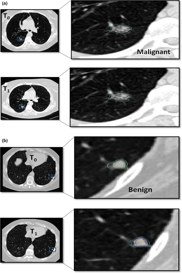
Segmentation boundary obtained by different semi‐automated methods used by the pteams shown for a representative nodule across two screening time points. Examples show (a) malignant nodule and (b) benign nodules. [Color figure can be viewed at wileyonlinelibrary.com]

2.5. Comparison of segmentation methods

In this preliminary effort, we compared different semi‐automated segmentation algorithms, operator expertise used by five research institutions to segment nodules across two consecutive time points. We proposed to compare tumor volume change estimates against single time point size or volume estimates, as the change measures by definition would offset any fixed biases that may exist in the methodologies followed by the teams.

In this effort, two teams (Team 1 and Team 2) used single seed point to initiate the algorithm, while others used a line (Team 4) or a 2D‐box (Team 3, Team 5) to contain the nodule region of interest. Team 1 used a single click and populated multiple seed point across different slices. Two other teams (Team 3 and 5) used active contour as their underlying segmentation approach with different set of customized initialization and region convergence procedures.

Team 2's prior work has shown the CIP segmentations had excellent agreement for large nodules with the expert radiologist drawn segmentation. But the CIP algorithm has not been optimized for smaller nodules and the regions often included normal surrounding tissues. We find Team 2's segmentation shows good concordance with other teams for large nodules (≥ 8 mm) and moderate concordance correlation for smaller nodules (< 8 mm).

Team 3 and Team 4 use manual over read on their semi‐automated segmentation workflow. Comparing un‐corrected segmentations between them showed lower concordance compared to other teams. The concordance between Team 3 and 4 improves using their corrected segmentations.

Inference of these methods poses significant challenges in comparing methodologies as each approach poses competing merits. In our approach, we compared the change in volume estimates against the diagnostic truth, which provides utility in the clinical imaging measurements. Table 2 contrasts different teams’ segmentation algorithms and seeding requirements.

Table 2.

Comparison of segmentation algorithms used by the participating teams with respective initialization requirement and reported comments

#	Institutions	Segmentation inputs	Software	Reported remarks
1	Team 1	Single click seeding. Automatically creates multiple clicks across slices.	Custom routines on Commercial platform 16	May include additional regions when nodules attached to pleura. Need manual over read.
2	Team 2	Single click seeding, automatically finds the centroid in a 3D region.	Open Source, 3D Slicer 17	Known issues with small nodules. Need manual over read
3	Team 3	2D box region	Custom routines based on C/C++.	Manual over read needed in some situations.
4	Team 4	Click and drag to: (a) create a seed point and (b) a line which is used to determine the threshold separating object from background.	Custom routines, based on ITK tools 29	It needs manual over read and editing.
5	Team 5	2D box region	Custom routines based on ITK tools 29	Manual over read in some situations.

3. Results

The size characteristics of the nodules for the selected 100 cases are presented in Table 1. The cohort demonstrates that the cases are not only were evenly distributed by patient diagnosis (cancer, not cancer), but they were evenly distributed between the smaller (< 8 mm diameter) group and the larger (≥ 8 mm diameter) nodule sized group. This table also shows that the smaller nodules tended to be benign, but were not exclusively so.

In terms of the overall agreement of segmentation results, Fig. 3(a) demonstrates that overall we found moderate overlap in the results across all teams with a mean DICE coefficient of 0.48 [Range: 0.12 to 0.97]. Figures 3(b) & 3(c) shows some examples of comparing segmentation results between: (a) two semi‐automated methods and (b) two semi‐automated methods without manual editing. For all the cases and segmentation methods, we computed the tumor volume across time points and compared the absolute and percent change in volumes. The Table 3 shows the concordance correlation coefficients for the study teams across all the nodules, regardless of size. Using absolute volume, we find a concordance correlation across all possible team comparison range between 0.56 and 0.95 with a median value of 0.83. We find the concordance correlation decreased to a range of 0.15–0.89, with a median of 0.55 for percent volume change. When the manually corrected segmentation was removed, the concordance correlation for absolute volume change ranged between 0.56 and 0.89 with a median of 0.80. While the percent volume change ranged from 0.15 to 0.83 with a median value of 0.44.

Figure 3.

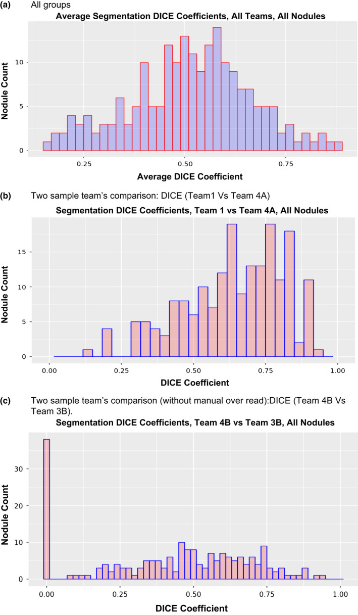
Similarity between segmentations, quantitatively measured by DICE coefficients, (a) All groups, (b) two groups using semi‐automated method, (c) two groups using semi‐automated methods without manual correction. [Color figure can be viewed at wileyonlinelibrary.com]

Table 3.

Concordance in the volume change computation between two consecutive screening time instances measured as absolute volume and percent volume change, compared across the teams. Categorized based on baseline size range and diagnosis at follow‐up: (A) All sizes (B) Below 8 mm, (C) Above 8 mm, (D) malignant nodule and (E) benign nodules. Concordance is measured by concordance correlation coefficient

(A) All size rage
CCC on Absolute volume (all sizes)
		Team 5	Team 4		Team 3		Team 2	Team 1
			None	With correction	None	With correction
Team 1		0.88	0.66	0.95	0.85	0.89	0.74	1
Team 2		0.82	0.56	0.75	0.83	0.77	1	0.74
Team 3	A (With correction)	0.92	0.76	0.92	0.94	1	0.77	0.89
	B (None)	0.89	0.67	0.89	1	0.94	0.83	0.85
Team 4	A (With correction)	0.89	0.71	1	0.89	0.92	0.75	0.95
	B (None)	0.78	1	0.71	0.67	0.76	0.56	0.66
Team 5		1	0.78	0.89	0.89	0.92	0.82	0.88

CCC on percent volume (all sizes)
		Team 5	Team 4		Team 3		Team 2	Team 1
			None	With correction	None	With correction
Team 1		0.83	0.24	0.78	0.55	0.8	0.46	1
Team 2		0.44	0.32	0.47	0.28	0.42	1	0.46
Team 3	A (With correction)	0.89	0.3	0.82	0.89	1	0.42	0.8
	B (None)	0.55	0.15	0.63	1	0.89	0.28	0.55
Team 4	A (With correction)	0.86	0.55	1	0.63	0.82	0.47	0.78
	B (None)	0.59	1	0.55	0.15	0.3	0.32	0.24
Team 5		1	0.59	0.86	0.55	0.89	0.44	0.83

(B) <8 mm
CCC on absolute volume (< 8 mm)
		Team 5	Team 4		Team 3		Team 2	Team 1
			None	With correction	None	With correction
Team 1		0.34	0.15	0.47	0.23	0.3	0.068	1
Team 2		0.037	−0.0038	0.056	0.061	0.038	1	0.068
Team 3	A (With correction)	0.61	0.34	0.5	0.61	1	0.038	0.3
	B (None)	0.64	0.27	0.5	1	0.61	0.061	0.23
Team 4	A (With correction)	0.69	0.24	1	0.5	0.5	0.056	0.47
	B (None)	0.38	1	0.24	0.27	0.34	−0.0038	0.15
Team 5		1	0.38	0.69	0.64	0.61	0.037	0.34

CCC on percent volume (< 8 mm)
		Team 5	Team 4		Team 3		Team 2	Team 1
			None	With correction	None	With correction
Team 1		0.92	0.0018	0.73	0.29	0.83	0.46	1
Team 2		0.24	−0.039	0.22	0.074	0.29	1	0.46
Team 3	A (With Correction)	0.88	−0.004	0.72	0.88	1	0.29	0.83
	B (None)	0.47	−0.015	0.5	1	0.88	0.074	0.29
Team 4	A (With Correction)	0.75	0.032	1	0.5	0.72	0.22	0.73
	B (None)	0.15	1	0.032	−0.015	−0.004	−0.039	0.0018
Team 5		1	0.15	0.75	0.47	0.88	0.24	0.92

(C) Long diameter, ≥ 8 mm
CCC on absolute volume (≥ 8 mm)
		Team 5	Team 4		Team 3		Team 2	Team 1
			None	With correction	None	With correction
Team 1		0.85	0.59	0.93	0.81	0.86	0.74	1
Team 2		0.85	0.54	0.76	0.85	0.79	1	0.74
Team 3	A (With Correction)	0.89	0.7	0.9	0.92	1	0.79	0.86
	B (None)	0.86	0.6	0.85	1	0.92	0.85	0.81
Team 4	A (With Correction)	0.85	0.64	1	0.85	0.9	0.76	0.93
	B (None)	0.73	1	0.64	0.6	0.7	0.54	0.59
Team 5		1	0.73	0.85	0.86	0.89	0.85	0.85

CCC on percent volume (≥ 8 mm)
		Team 5	Team 4		Team 3		Team 2	Team 1
			None	With correction	None	With correction
Team 1		0.75	0.3	0.8	0.61	0.76	0.55	1
Team 2		0.8	0.58	0.77	0.81	0.86	1	0.55
Team 3	A (With correction)	0.88	0.6	0.88	0.89	1	0.86	0.76
	B (None)	0.73	0.46	0.75	1	0.89	0.81	0.61
Team 4	A (With correction)	0.95	0.69	1	0.75	0.88	0.77	0.8
	B (None)	0.67	1	0.69	0.46	0.6	0.58	0.3
Team 5		1	0.67	0.95	0.73	0.88	0.8	0.75

(D) All benign cases
CCC on absolute volume (benign nodules)
		Team 5	Team 4		Team 3		Team 2	Team 1
			None	With correction	None	With correction
Team 1		0.92	0.75	0.94	0.89	0.96	0.63	1
Team 2		0.67	0.48	0.63	0.62	0.62	1	0.63
Team 3	A (With correction)	0.95	0.8	0.95	0.95	1	0.62	0.96
	B (None)	0.89	0.91	0.78	1	0.95	0.62	0.89
Team 4	A (With correction)	0.92	0.71	1	0.91	0.95	0.63	0.94
	B (None)	0.77	1	0.72	0.78	0.8	0.48	0.75
Team 5		1	0.77	0.92	0.89	0.95	0.67	0.92

CCC on percent volume (benign nodules)
		Team 5	Team 4		Team 3		Team 2	Team 1
			None	With correction	None	With correction
Team 1		0.21	0.0034	−0.052	0.037	0.32	0.019	1
Team 2		−0.11	−0.0096	−0.0096	0.15	−0.036	1	0.019
Team 3	A (With correction)	0.16	0.059	0.059	0.21	1	−0.036	0.32
	B (None)	0.22	0.45	0.45	1	0.21	0.15	0.037
Team 4	A (With correction)	0.14	0.018	1	0.45	0.059	−0.0096	−0.052
	B (None)	0.1	1	0.018	−0.0081	0.042	−0.072	0.0034
Team 5		1	0.14	0.14	0.22	0.16	−0.11	0.21

(E) All malignant cases
CCC on absolute volume (malignant nodules)
		Team 5	Team 4		Team 3		Team 2	Team 1
			None	With correction	None	With correction
Team 1		0.86	0.61	0.94	0.83	0.87	0.75	1
Team 2		0.86	0.55	0.78	0.88	0.81	1	0.75
Team 3	A (With correction)	0.9	0.71	0.91	0.93	1	0.81	0.87
	B (None)	0.88	0.62	0.87	1	0.93	0.88	0.83
Team 4	A (With correction)	0.87	0.68	1	0.87	0.91	0.78	0.94
	B (None)	0.76	1	0.68	0.62	0.72	0.55	0.61
Team 5		1	0.76	0.87	0.88	0.9	0.86	0.86

CCC on percent volume (malignant nodules)
		Team 5	Team 4		Team 3		Team 2	Team 1
			None	With correction	None	With correction
Team 1		0.83	0.23	0.75	0.49	0.77	0.51	1
Team 2		0.51	0.66	0.52	0.27	0.48	1	0.51
Team 3	A (With correction)	0.89	0.3	0.8	0.89	1	0.48	0.77
	B (None)	0.51	0.12	0.57	1	0.89	0.27	0.49
Team 4	A (With correction)	0.85	0.59	1	0.57	0.8	0.52	0.75
	B (None)	0.63	1	0.59	0.12	0.3	0.66	0.23
Team 5		1	0.63	0.85	0.51	0.89	0.51	0.83

To evaluate the effects of nodule size on the results, we repeated the analysis to compare volume estimates across time intervals for nodules less than 8 mm in longest diameter and greater than or equal to 8 mm measured at baseline. Table 3(B) shows that we find the concordance correlation for < 8 mm, ranged between −0.0038 and 0.385 for absolute volume with a median of 0.3 and a range of −0.039 to 0.59 with a median of 0.29 for percent volume change. Removing manually corrected cases, the absolute volume ranged between −0.0038 and 0.27 with a median of 0.26. The percent volume ranged between −0.039 and 0.38 with a median of 0.27. For larger nodules (≥8 mm diameter), Table 3(C) shows the concordance improves, with the absolute volume values ranged between 0.54 and 0.85 with a median of 0.85, while the percent volume ranged between 0.3 and 0.78 with a median of 0.75. When the manually corrected cases were removed the concordance for absolute volume ranged 0.54–0.80 with a median of 0.78, while percent volume ranged 0.3–0.67 with a median of 0.61.

We then repeated the analysis by partitioning the cohort with diagnostic labels as shown in Tables 3(D) & 3(E). For benign nodules, the absolute volume change had a concordance ranged between 0.48 and 0.91 with a median of 0.8, while percent volume was between 0.099 and 0.11 with a median of 0.059. After manual correction the concordance, the correlation ranged between 0.4 and 0.82 with a median of 0.76 for absolute volume. The percent volume change ranged between 0.028 and 0.11 with a median of 0.037. While for malignant nodules, the absolute volume estimates concordance range between 0.55 and 0.87 with a median of 0.86. The percent volume measure did not show any improvement, which had a range of 0.12–0.63 with a median of 0.5.

The volumes estimate does not improve after removing manually corrected cases, the absolute volume ranged 0.55–0.81 with a median of 0.797, while the percent volume ranged between 0.12 and 0.51 with a median of 0.5. Figure 4 shows comparison of volume estimates between two selected sites.

Figure 4.

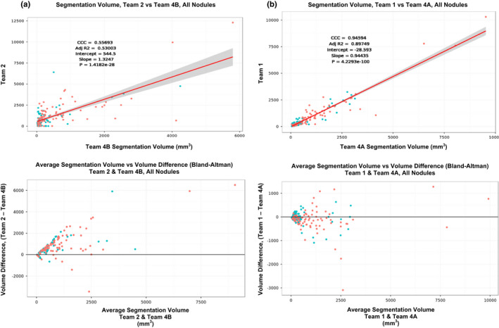
Comparison of volume estimate between the teams using scatter plots and difference plots (Bland‐Altman plot): (a) Between Team 2 and Team 4B, (b) Team 1 Vs Team 4A. [Color figure can be viewed at wileyonlinelibrary.com]

We used change in volume estimates, both absolute change and percent change, for the teams to predict the malignancy status of the nodules. For absolute volume change, the area under the receiver operator curve ranged between 0.65 and 0.89 across methods. For percent change in volume, the prediction scores ranged between 0.64 and 0.86 across methods. For the cohort of nodules < 8 mm, the AUC was between 0.57 and 0.80 for absolute volume and the AUC was in the range between 0.59 and 0.77 for percent volume. While for the larger nodules (longest diameter ≥ 8 mm), the AUC ranged between 0.75 and 0.9 using absolute volume and using percent volume the AUC ranged between 0.74 and 0.89. Detailed prediction results are presented in Table 4. The Fig. 5 shows the AUC using absolute volume and percent volume computed between the screening intervals for the teams.

Table 4.

Prediction performance (Area under the curve, AUC) of malignant nodule characterization using volume estimates (absolute volume change & percent volume change) obtained from segmentations provided by the teams. Results categorized based on (A) All sizes (B) Below 8 mm, (C) Above 8 mm

(A) All size rage
ROC characterization
		Absolute volume		Percent volume
		AUC (95% CI)	#Samples	AUC (95% CI)	#Samples
Team 1		0.82 [0.78, 0.86]	100	0.82 [0.78, 0.86]	100
Team 2		0.78 [0.73, 0.83]	100	0.73 [0.68,0.78]	98
Team 3	A (With correction)	0.89 [0.86,0.92]	100	0.86 [0.82,0.90]	100
	B (None)	0.86 [0.82,0.90]	100	0.82 [0.78,0.86]	100
Team 4	A (With correction)	0.83 [0.79,0.87]	100	0.82 [0.78,0.86]	100
	B (None)	0.65 [0.59,0.71]	80	0.64 [0.58,0.70]	80
Team 5		0.76 [0.73, 0.83]	100	0.76 [0.72,0.81]	100
Longest diameter
Radiologist measured		0.78 [0.73,0.83]		0.81 [0.85, 0.77]

(B) Diameter < 8 mm
ROC characterization
		Absolute volume		Percent volume
		AUC	#Samples	AUC	#Samples
Team 1		0.80	50	0.77	50
Team 2		0.63	49	0.60	49
Team 3	A (With correction)	0.78	50	0.75	50
	B (None)	0.80	50	0.77	50
Team 4	A (With correction)	0.76	50	0.77	50
	B (None)	0.57	39	0.59	39
Team 5		0.79	50	0.76	50

(C) Long diameter ≥ 8 mm
ROC characterization
		Absolute volume		Percent volume
		AUC	#Samples	AUC	#Samples
Team 1		0.83	49	0.81	49
Team 2		0.84	49	0.84	49
Team 3	With correction	0.90	49	0.92	49
	None	0.90	49	0.88	49
Team 4	With correction	0.88	49	0.89	49
	None	0.75	40	0.74	40
Team 5		0.81	49	0.76	49

Figure 5.

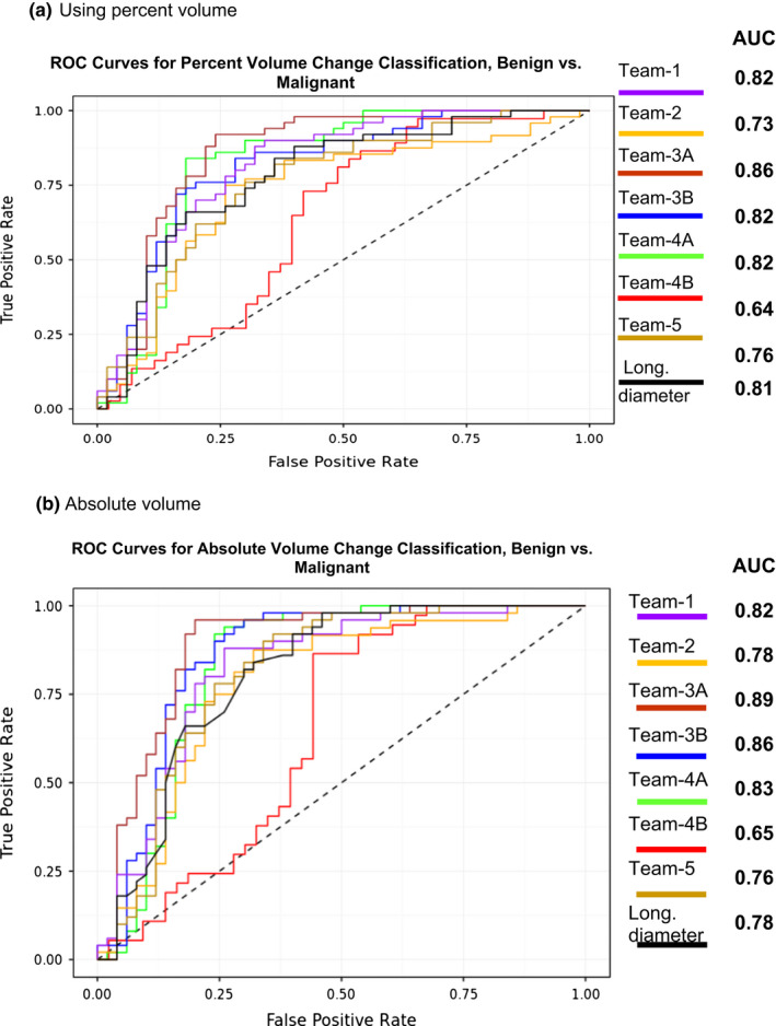
Receiver operator curves (ROC) across teams to predict nodules malignancy using, (a) percent volume change and (b) absolute volume change. [Color figure can be viewed at wileyonlinelibrary.com]

When considering the entire nodule size range, Team 1 and 2 showed statistically comparable AUCs with overlapping confidence range [0.78, 0.86] and [0.73, 0.83]. Team 3A's (corrected) AUC was superior to any other teams with a confidence limits of [0.86, 0.92], while their uncorrected AUC showed slightly lower performance that was comparable with other teams [0.82, 0.90]. Team 4's corrected estimates’ AUC was in the range of [0.79, 0.87], while their uncorrected AUC showed lower average AUC with a confidence range of [0.59, 0.71]. Team 5's average AUC was in the middle compared to others uncorrected estimates, with confidence limits of [0.72, 0.83]. It is interesting to note that, most semi‐automated AUC's showed slightly superior performance compared to radiologist delineated contours, whose average AUC was 0.78 with a confidence range of [0.73, 0.83]. When nodule sizes were restricted to smaller size (< 8 mm), Team 1, 3 and 5's predictor AUC confidence ranges are comparable. Teams 2 and 4 AUC performances were lower compared to other teams.

4. Discussion

In this retrospective study, we compared the segmentation results across five different institutions with varied algorithmic approaches to delineate the pulmonary nodules in screening setting. We evaluated the concordance between the participating teams’ estimates of nodule volume change across two time intervals and used the measure to predict the malignancy status. We then compared prediction results using the individual volume change estimates obtained from the segmentations provided by the institutions. There have been number of studies that showed volume of pulmonary nodules to be a better estimate to assess growth over time and few studies have shown its ability to predict malignancy.^{27, 30, 31}

In our current study, we find the concordance of absolute volume across time points between the teams (median of 0.83) is better than the percent volume change, median concordance of 0.55. While the concordance drops further (0.80 for absolute volume and 0.44 percent volume) after removing manually corrected cases. The segmentation difference across time points is higher in the percent volume change compared to absolute volume change, which we believe is exacerbated by a factor defined by the in‐plane and inter‐slice resolution. As expected the concordance across teams was lower for smaller nodules (< 8 mm), median value between teams was 0.31 and 0.29 for absolute and percent volume change, respectively. This was expected as the delineation of missed or added boundaries is greater for smaller nodules, where a region of about 16 × 16 pixels (about 0.5 × 0.5 mm, in‐plane resolution) is relatively smaller regions, which increases the probability of errors. As expected, the concordance between the teams is higher for larger size nodules of ≥ 8 mm (median between teams was 0.85 and 0.75 for absolute volume and % volume change). We find the concordance between the teams is lower for benign nodules (median between the groups of 0.8), while it improves for malignant nodules (median between the groups of 0.86). It is clear that the malignant nodules are larger in size compared to benign ones (see Table 1).

The Federal Drug Administration (FDA) sponsored studies have created lung phantom with artificial nodules of different shapes for the community to compare size estimates.³² Recently these nodules were given to a clinical radiologist to assess the sizes and volume estimation, a variability of 3.9 to 28% has been reported, they have shown a higher variability for smaller nodules.³³ Interestingly, the authors report a repeatability coefficient in the size estimation to be in the range of 6.2% to 40%.

We further use the volume change estimates from each of the teams to assess the malignancy prediction. We find the prediction AUC was high (median of 0.82) using all the nodules, while the AUC was slightly lower for smaller size (<8 mm) nodules, median AUC of 0.8 compared to large size nodules (≥8 mm), median AUC of 0.84. We find most teams were able to predict malignancy with fairly higher AUC, though the concordance correlation of volume change between the groups shows a wide range.

Estimation the volume of pulmonary nodules across centers with varied imaging expertise, algorithms and software implementation has been a persistent issue in medical imaging. In a recent community driven challenge ³⁴ organized by Quantitative Imaging Biomarker Alliance (QIBA), proposed to use phantoms as their study subjects. The study reports 84% of volume measurement were within 15% of the true volume and the variability ranges from 66% to 93% across algorithms. While the 61% of volume measurements for all tumors ranged from 37% to 84%. QIBA study claims algorithm type did not affect bias substantially and reports algorithm precision was notably better as tumor size increases and worsen when the nodules were irregular. They also report 18.4% overall repeatability coefficient for their study.

Our study effort was motivated by the clinical use of the tumor measurement, especially change in volume across time points which may be relevant for screening exams. There is certainly high clinical benefit to find concordance in measuring change in volume estimate across institutions that use different delineation algorithms. We used real patient images with no true estimate of tumor volume.

The community could also benefit in adopting variability standards in the use of outcome prediction that was reported by comparing different sites, expertise and with the use of imaging algorithms tested on a diverse patient cohorts obtained from the NLST trial. The teams agreed on certain limitations in the group effort. These included allowing multiple independent user inputs to seed segmentation algorithms as well as allowing variability in the location and size of the seeds (length of the bounding box, length of the seed line).

Best Practices for volume measurements and lessons learnt:

• It is important to avoid biases in size and volume measurements. Some common biases include use of any clinical diagnostics and or radiological observational intuition prior to delineate the region of interest. In a clinical setting, most focus is to improve true positive detection. Prior diagnostic information strongly impact true assessment of nodules size or volume measurements.

• Most often clinical radiologists are influenced by the nodules shape characteristics. Recently, some of these shape characteristics have been used to provide clinical risk decision.³⁵ It becomes imperative that region of interest is delineated prior to assessment of shape characteristics.

• Some known variations are attributed to the segmentation algorithms and the imaging suites methodologies, which show differences due to numerical rounding and different ways to deal with boundary voxels.

• Variability due to nodules morphology, density variation (including nodule solidity) affects the segmentation algorithms performance.

• There are few others variability sources caused by scanner parameters and reconstruction methods which influence the image intensity. Where small regional difference could lead to large size/volume changes.

5. Conclusion

In this study, we compared the volume assessment of pulmonary nodules across two screening interval between five institutions. We find a range of concordance between institutions that used varied software and clinical expertise. We find that prediction of malignancy shows acceptable values across institutions. The nodules predictions across the teams are higher for larger nodules compared to smaller nodules. We find variability in volume change is well reproducible across algorithms (median concordance over 0.75).

Conflict of interest

Y.B., A.B., J.K.C., L.H., J.Z., H.Y., S.Y., H.A., D.C., K.C., H.P.C., C.F., A.G., D.G. None to disclose. BZ: no conflicts related to this study. Receives royalties from Varian Medical Systems and Keosys Medical Imaging companies. MMG: no conflicts related to this study. UCLA Department of Radiology has a Master Research Agreement with Siemens Healthineers, Erlangen, Germany. SN: no conflicts related to this study. Consultant in Carestream Inc, Scientific advisor for: EchoPixel Inc, Fovia Inc, Radlogic,Inc. RJG: no conflicts related to this study. Investor in Health myne Inc. Moffitt cancer center has research agreement with Health Myne.

References

- 1. Siegel RL, Miller KD, Jemal A. Cancer statistics. CA Cancer J Clin. 2016;66:7–30. [DOI] [PubMed] [Google Scholar]
- 2. Aberle DR, Berg CD, Black WC, et al. The national lung screening trial: overview and study design. Radiology. 2011;258:243–253. [DOI] [PMC free article] [PubMed] [Google Scholar]
- 3. Baecke E, de Koning HJ, Otto SJ, van Iersel CA, van Klaveren RJ. Limited contamination in the Dutch‐Belgian randomized lung cancer screening trial (NELSON). Lung Cancer. 2010;69:66–70. [DOI] [PubMed] [Google Scholar]
- 4. Aberle DR, Adams AM, Berg CD, et al. Reduced lung‐cancer mortality with low‐dose computed tomographic screening. New Engl J Med. 2011;365:395–409. [DOI] [PMC free article] [PubMed] [Google Scholar]
- 5. Center for medicare and medicaid , Department of Health and Human Services, USA; 2015. Available from: www.cms.gov/medicare-coverage-database/details/nca-decisionmemo.aspx?NCAId=274&NcaName=Screening+for+Lung+Cancer+with+Low+Dose+Computed+Tomography+(LDCT)&TimeFram=7&DocType=All&bc=AQAAIAAAAgAAAA%3d%3d&;
- 6. Radiology ACo . Lung imaging resource; 2014. Available from: https://www.acr.org/Quality-Safety/Resources/Lung-Imaging-Resources
- 7. Patz EF Jr, Pinsky P, Gatsonis C, et al. Overdiagnosis in low‐dose computed tomography screening for lung cancer. JAMA Intern Med. 2014;174:269–274. [DOI] [PMC free article] [PubMed] [Google Scholar]
- 8. Center for medicare and medicaid . Department of Health and Human Services, USA; 2015. Available from: https://www.cms.gov/medicare-coverage-database/details/nca-decisionmemo.aspx?NCAId=274&NcaName=Screening+for+Lung+Cancer+with+Low+Dose+Computed+Tomography+(LDCT)&TimeFram=7&DocType=All&bc=AQAAIAAAAgAAAA%3d%3d&
- 9. Mehta HJ, Ravenel JG, Shaftman SR, et al. The utility of nodule volume in the context of malignancy prediction for small pulmonary nodules. Chest. 2014;145:464–472. [DOI] [PMC free article] [PubMed] [Google Scholar]
- 10. Ko JP, Berman EJ, Kaur M, et al. Pulmonary nodules: growth rate assessment in patients by using serial CT and three‐dimensional volumetry. Radiology. 2012;262:662–671. [DOI] [PMC free article] [PubMed] [Google Scholar]
- 11. Henschke CI, Yankelevitz DF, Yip R, et al. Lung cancers diagnosed at annual CT screening: volume doubling times. Radiology. 2012;263:578–583. [DOI] [PMC free article] [PubMed] [Google Scholar]
- 12. Armato SG 3rd, McLennan G, Bidaut L, et al. The lung image database consortium (LIDC) and image database resource initiative (IDRI): a completed reference database of lung nodules on CT scans. Med Phys. 2011;38:915–931. [DOI] [PMC free article] [PubMed] [Google Scholar]
- 13. Petrick N, Kim HJ, Clunie D, et al. Comparison of 1D, 2D, and 3D nodule sizing methods by radiologists for spherical and complex nodules on thoracic CT phantom images. Acad Radiol. 2014;21:30–40. [DOI] [PubMed] [Google Scholar]
- 14. Cagnon CH, Cody DD, McNitt‐Gray MF, Seibert JA, Judy PF, Aberle DR. Description and implementation of a quality control program in an imaging‐based clinical trial. Acad Radiol. 2006;13:1431–1441. [DOI] [PubMed] [Google Scholar]
- 15. Larobina M, Murino L. Medical image file formats. J Digit Imaging. 2014;27:200–206. [DOI] [PMC free article] [PubMed] [Google Scholar]
- 16. Schonmeyer R, Athelogou M, Sittek H, et al. Cognition Network Technology prototype of a CAD system for mammography to assist radiologists by finding similar cases in a reference database. Int J Comput Assist Radiol Surg. 2011;6:127–134. [DOI] [PubMed] [Google Scholar]
- 17. Fedorov A, Beichel R, Kalpathy‐Cramer J, et al. 3D slicer as an image computing platform for the quantitative imaging network. Magn Reson Imaging. 2012;30:1323–1341. [DOI] [PMC free article] [PubMed] [Google Scholar]
- 18. Raul San Jose E, James CR, Rola H, Jorge O, Alejandro AD, George RW. Chest imaging platform: an open‐source library and workstation for quantitative chest imaging. C66 lung imaging II: new probes and emerging technologies: American Thoracic Society, 2015; p. A4975‐A.
- 19. Tan Y, Schwartz LH, Zhao B. Segmentation of lung lesions on CT scans using watershed, active contours, and Markov random field. Med Phys. 2013;40:043502. [DOI] [PMC free article] [PubMed] [Google Scholar]
- 20. Weasis . Weasis open source tools; 2017. Available from: https://dcm4che.atlassian.net/wiki/display/WEA/Home
- 21. Gu Y, Kumar V, Hall LO, et al. Automated delineation of lung tumors from CT images using a single click ensemble segmentation approach. Pattern Recogn. 2013;46:692–702. [DOI] [PMC free article] [PubMed] [Google Scholar]
- 22. Way TW, Hadjiiski LM, Sahiner B, et al. Computer‐aided diagnosis of pulmonary nodules on CT scans: segmentation and classification using 3D active contours. Med Phys. 2006;33:2323–2337. [DOI] [PMC free article] [PubMed] [Google Scholar]
- 23. Brown MS, McNitt‐Gray MF, Pais R, et al. CAD in clinical trials: current role and architectural requirements. Comput Med Imaging Graph. 2007;31:332–337. [DOI] [PubMed] [Google Scholar]
- 24. Caselles V, Kimmel R, Sapiro G. Geodesic active contours. Int J Comput Vision. 1997;22:61–79. [Google Scholar]
- 25. Krishnan K, Ibanez L, Turner WD, Jomier J, Avila RS. An open‐source toolkit for the volumetric measurement of CT lung lesions. Opt Express. 2010;18:15256–15266. [DOI] [PubMed] [Google Scholar]
- 26. Yip SSF, Parmar C, Blezek D, et al. Application of the 3D slicer chest imaging platform segmentation algorithm for large lung nodule delineation. PLoS ONE. 2017;12:e0178944. [DOI] [PMC free article] [PubMed] [Google Scholar]
- 27. Zhao YR, vanOoijen PM , Dorrius MD, et al. Comparison of three software systems for semi‐automatic volumetry of pulmonary nodules on baseline and follow‐up CT examinations. Acta Radiol. 2014;55:691–698. [DOI] [PubMed] [Google Scholar]
- 28. Dice L. Measures of the amount of ecologic association between species. Ecol Soc Am. 1945;26:297–302. [Google Scholar]
- 29. ITK . Imaging ToolKit; 2017. Available from: https://itk.org/
- 30. Han D, Heuvelmans MA, Oudkerk M. Volume versus diameter assessment of small pulmonary nodules in CT lung cancer screening. Transl Lung Cancer Res. 2017;6:52–61. [DOI] [PMC free article] [PubMed] [Google Scholar]
- 31. Liang M, Yip R, Tang W, et al. Variation in screening CT‐detected nodule volumetry as a function of size. AJR Am J Roentgenol. 2017;209:304–308. [DOI] [PubMed] [Google Scholar]
- 32. Gavrielides MA, Zeng R, Kinnard LM, Myers KJ, Petrick N. Information‐theoretic approach for analyzing bias and variance in lung nodule size estimation with CT: a phantom study. IEEE Trans Med Imaging. 2010;29:1795–1807. [DOI] [PubMed] [Google Scholar]
- 33. Li Q, Gavrielides MA, Sahiner B, Myers KJ, Zeng R, Petrick N. Statistical analysis of lung nodule volume measurements with CT in a large‐scale phantom study. Med Phys. 2015;42:3932–3947. [DOI] [PMC free article] [PubMed] [Google Scholar]
- 34. Athelogou M, Kim HJ, Dima A, et al. Algorithm variability in the estimation of lung nodule volume from phantom CT scans: results of the QIBA 3A public challenge. Acad Radiol. 2016;23:940–952. [DOI] [PMC free article] [PubMed] [Google Scholar]
- 35. McWilliams A, Tammemagi MC, Mayo JR, et al. Probability of cancer in pulmonary nodules detected on first screening CT. New Engl J Med. 2013;369:910–919. [DOI] [PMC free article] [PubMed] [Google Scholar]