Quantifying Publication Bias in Meta-Analysis

Summary

Publication bias is a serious problem in systematic reviews and meta-analyses, which can affect the validity and generalization of conclusions. Currently, approaches to dealing with publication bias can be distinguished into two classes: selection models and funnel-plot-based methods. Selection models use weight functions to adjust the overall effect size estimate and are usually employed as sensitivity analyses to assess the potential impact of publication bias. Funnel-plot-based methods include visual examination of a funnel plot, regression and rank tests, and the nonparametric trim and fill method. Although these approaches have been widely used in applications, measures for quantifying publication bias are seldom studied in the literature. Such measures can be used as a characteristic of a meta-analysis; also, they permit comparisons of publication biases between different meta-analyses. Egger’s regression intercept may be considered as a candidate measure, but it lacks an intuitive interpretation. This article introduces a new measure, the skewness of the standardized deviates, to quantify publication bias. This measure describes the asymmetry of the collected studies’ distribution. In addition, a new test for publication bias is derived based on the skewness. Large sample properties of the new measure are studied, and its performance is illustrated using simulations and three case studies.

1. Introduction

Meta-analysis has become a powerful and widely-used tool to integrate findings from different studies and inform decision making in evidence-based medicine (Sutton and Higgins, 2008). However, the chance of a study being published by a scientific journal is frequently associated with the statistical significance of its results: more significant findings are more likely to be published, causing publication bias in meta-analysis of published studies (Begg and Berlin, 1988; Stern and Simes, 1997; Kicinski et al., 2015). Detecting publication bias is a critical problem because such bias may lead to incorrect conclusions of systematic reviews (Sutton et al., 2000).

One class of approaches to detecting publication bias is based on selection models. These approaches typically use the weighted distribution theory to model the selection (i.e., publication) process and develop estimation procedures that account for the selection process; see, e.g., Dear and Begg (1992), Hedges (1992), and Silliman (1997a,b). Sutton et al. (2000) provide a comprehensive review. The selection models are usually complicated, limiting their applicability. Moreover, they incorporate weight functions in an effort to correct publication bias, but strong and largely untestable assumptions are often made (Sutton et al., 2000). Therefore, the validity of their adjusted results may be doubtful, and these methods are usually employed as sensitivity analyses.

Another class of methods for publication bias is based on a funnel plot, which usually presents effect sizes plotted against their standard errors or precisions (the inverse of standard errors) (Light and Pillemer, 1984; Sterne and Egger, 2001). In the presence of publication bias, the funnel plot is expected to be skewed; see the illustrative example in Figure 1. One may intuitively assess publication bias by examining the asymmetry of the funnel plot; however, the visual examination is usually subjective. Various statistical tests have been proposed for publication bias in the funnel plot, such as Begg’s rank test (Begg and Mazumdar, 1994) and Egger’s regression test (Egger et al., 1997) and its extensions (e.g., Macaskill et al., 2001; Rothstein et al., 2005; Harbord et al., 2006; Peters et al., 2006). The rank test examines the correlation between the effect sizes and their corresponding sampling variances; a strong correlation implies publication bias. Egger’s test regresses the standardized effect sizes on their precisions; in the absence of publication bias, the regression intercept is expected to be zero. Note that this regression is equivalent to a weighted regression of the effect sizes on their standard errors, weighted by the inverse of their variances; the weighted regression’s slope, instead of the intercept, is expected to be zero in the absence of publication bias (Rothstein et al., 2005). The weighted regression version of the test is popular among meta-analysts, probably because it directly links the effect sizes to their standard errors without the standardization process. However, this article considers only the original version of regression as in Egger et al. (1997), since it is closely related to commonly-used meta-analysis models; see Section 2 for details. In addition, another attractive method is the trim and fill method, which not only tests for publication bias but also adjusts the estimated overall effect size (Duval and Tweedie, 2000a,b). Although these publication bias tests have been widely used in meta-analysis applications, they may suffer from inflated type I error rate or poor power in certain simulation settings (Sterne et al., 2000; Terrin et al., 2003; Peters et al., 2006, 2007; Rücker et al., 2008).

Figure 1.

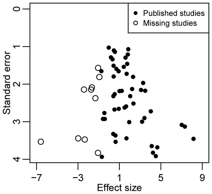
The funnel plot of a simulated meta-analysis containing 60 studies. The 10 studies with the most negative effect sizes were suppressed due to publication bias, and the remaining 50 studies were “published”.

Besides detecting publication bias using selection models and funnel-plot-based methods, it is also important to quantify publication bias using measures that permit comparisons between different meta-analyses. A candidate measure is the intercept of the regression test (Egger et al., 1997). However, as a measure of asymmetry of the collected study results, the regression intercept lacks a clear interpretation; for example, it is difficult to provide a range guideline to determine mild, moderate, or substantial publication bias based on the regression intercept. Due to this limitation, meta-analysts usually report the p-value of Egger’s regression test, but not the magnitude of the intercept. We will show that the regression intercept basically estimates the average of study-specific standardized deviates; it does not account for the shape of the deviates, which is skewed in the presence of publication bias. This may limit the statistical power of Egger’s regression test.

This article introduces an alternative measure to quantify publication bias, the skewness of the standardized deviates. The new measure not only has an intuitive interpretation as the asymmetry of the collected study results but also can serve as a test statistic. The large sample properties of the new measure are studied. We also evaluate its performance using simulations and three actual meta-analyses published in the Cochrane Database of Systematic Reviews.

2. Notation and the regression test

Suppose a meta-analysis collects n studies; each study reports an effect size y_i (e.g., log odds ratio for binary outcomes) and its within-study variance $s_i^2$, due to sampling error (i = 1, …, n). If the collected studies are deemed homogeneous, sharing a common underlying true effect size μ, then the fixed-effect model is customarily used, specified by $y_i~N(\mu ,s_i^2)$. The studies are heterogeneous if they have different underlying effect sizes μ_i; the corresponding random-effects model assumes $y_i~N(\mu ,s_i^2)$ and μ_i ~ N(μ, τ²), where τ² is the between-study variance and μ is interpreted as the overall mean effect size (Borenstein et al., 2010). The random-effects model reduces to the fixed-effect model by setting τ² = 0.

To detect publication bias, Egger et al. (1997) proposed a regression test, regressing the standardized effect sizes (y_i/s_i) on the corresponding precisions (1/s_i); that is,

$$y_i/s_i=\alpha +\mu ·1/s_i+{\epsilon }_i,{\epsilon }_i\stackrel{\text{iid}}{\sim }N(0,{\sigma }^2).$$

Egger’s regression test transforms the original null hypothesis, H₀: no publication bias, to testing $H_0^{\prime }$: the regression intercept is zero. Alternatively, in the presence of noticeable heterogeneity between studies, we may slightly modify Egger’s test by using the marginal standard deviations to produce the regression predictors and responses under the random-effects model. Note that the random-effects model can be written marginally as y_i = μ+δ_i+ξ_i, where ${\delta }_i\stackrel{\text{iid}}{\sim }N(0,{\tau }^2)$ is the random effect and ${\xi }_i~N(0,s_i^2)$ is the sampling error in study i. Dividing by the marginal standard deviation ${(s_i^2+{\tau }^2)}^{1/2}$, we have the following modified regression test:

$$y_i{(s_i^2+{\tau }^2)}^{-1/2}=\alpha +\mu {(s_i^2+{\tau }^2)}^{-1/2}+{\epsilon }_i,{\epsilon }_i\stackrel{\text{iid}}{\sim }N(0,{\sigma }^2).$$ (1)

Like Egger’s test, the intercept α is zero under the true model; in the presence of publication bias, it departs from zero. The overall mean effect size μ becomes the regression slope. Also, σ² allows potential under- or over-dispersion of the errors. In practice, heterogeneity is routinely assessed using the Q or I² statistic (Whitehead and Whitehead, 1991; Higgins and Thompson, 2002; Higgins et al., 2003; Borenstein et al., 2010), and the between-study variance can be estimated as τ̂² using the method of moments or the maximum restricted likelihood method (DerSimonian and Laird, 1986; Normand, 1999). If heterogeneity is not significant, then setting τ² = 0 reduces Equation (1) to Egger’s original test. Since the heterogeneity frequently appears in meta-analyses (Higgins, 2008), this article will introduce publication bias measures based on the modified regression test.

Let the least squares estimates of the regression coefficients in model (1) be α̂ and μ̂. The estimated regression intercept is essential in the regression test; we denote this statistic as

$$T_I=\widehat{\alpha }.$$

Under the null hypothesis, T_I divided by its standard error follows the t-distribution with degrees of freedom n − 2, which gives the p-value of the regression test, denoted as P_I. Since the standardized effect sizes are unit-free, the estimated regression intercept T_I is also unit-free. Therefore, T_I can serve as a measure for quantifying publication bias (Egger et al., 1997). However, the regression intercept T_I lacks an intuitive interpretation for the asymmetry of the collected study results. Meta-analysts usually report only the p-value of the regression test, not the magnitude of T_I, to describe the severity of publication bias.

3. Skewness and skewness-based test

The regression test does not fully describe the asymmetry of the collected study results. By linear regression theory, the estimated intercept can be expressed as $T_I=n^{-1}{\sum }_{i=1}^n{\widehat{d}}_i$, where

$${\widehat{d}}_i=\frac{y_i-\widehat{\mu }}{\sqrt{s_i^2+{\widehat{\tau }}^2}}$$

is an estimate of the study-specific standardized deviate $d_i=(y_i-\mu ){(s_i^2+{\tau }^2)}^{-1/2}$. Therefore, the regression intercept T_I only reflects the average of the standardized deviates. To better test and quantify publication bias, we further consider the shape of the d_i’s.

Note that d_i = α+ε_i, so the standardized deviates d_i are distributed with the same shape as the errors ε_i. To test the original H₀, we may alternatively test $H_0^{″}:\alpha =0$ and ${\epsilon }_i\stackrel{\text{iid}}{\sim }N(0,{\sigma }^2)$vs. $H_1^{″}:\alpha \ne 0$ or ε_i’s are iid from a skewed distribution with mean zero. Clearly, $H_0^{″}$ is stronger than the null hypothesis $H_0^{\prime }$ of Egger’s test, but it is still a necessary condition if the original null hypothesis H₀ holds. Hence, the statistical power should be enhanced by testing $H_0^{″}$ compared to testing $H_0^{\prime }$.

In the statistical literature, skewness has long been used as a descriptive quantity for the asymmetry of a distribution (MacGillivray, 1986), but it is fairly novel in the literature of meta-analysis. To assess publication bias in meta-analysis, we may quantify the asymmetry of ε = (ε₁, …, ε_n)^T by the skewness, calculated as Skew(ε) = m₃/s³, where $s={\{{(n-1)}^{-1}{\sum }_{i=1}^n{({\epsilon }_i-\overline{\epsilon })}^2\}}^{1/2}$ is the sample standard deviation, $m_3=n^{-1}{\sum }_{i=1}^n{({\epsilon }_i-\overline{\epsilon })}^3$ is the sample third central moment, and $\overline{\epsilon }=n^{-1}{\sum }_{i=1}^n{\epsilon }_i$. In practice, we may replace the unknown errors ε with the regression residuals ε̂ = (ε̂₁, …, ε̂_n)^T, where ε̂_i = d̂_i − T_I. Denote the sample skewness of the errors as

$$T_S=\text{Skew}\left(\widehat{\mathit{\epsilon }}\right),$$

which we propose as an alternative measure of publication bias. We will show that T_S is a consistent estimate of the true skewness.

The sample skewness T_S can take any real value. A symmetric distribution (i.e., publication bias is not present) has zero skewness. A noticeably large positive skewness indicates that the right tail of standardized deviates’ distribution is longer than its left tail. Therefore, some studies on the left side in the funnel plot (i.e., those with negative effect sizes) might be missing due to publication bias. In this situation, the regression intercept T_I is also expected to be positive. On the other hand, a large negative skewness implies that some studies may be missing on the right side. A common but rough rule of interpreting skewness is as follows. If the skewness is less than 0.5 in absolute magnitude, the distribution of the standardized deviates is approximately symmetric; the skewness is deemed considerable if it is between 0.5 and 1 in absolute magnitude, and it may be substantial if its absolute value is greater than 1. To interpret the skewness more rigorously, we study its large sample properties.

Denote β_k = E(ε₁ − β)^k as the kth central moment of the errors ε_i, where β = E(ε₁) = 0, and the sample kth central moment is $m_k=n^{-1}{\sum }_{i=1}^n{\left({\epsilon }_i-\overline{\epsilon }\right)}^k$. Then the true skewness of the errors is $\gamma ={\beta }_3/{\beta }_2^{3/2}$. In addition, let ${\widehat{m}}_k=n^{-1}{\sum }_{i=1}^n{\left({\widehat{\epsilon }}_i-\overline{\widehat{\epsilon }}\right)}^k$ be the sample kth central moment after plugging in the known residuals ε̂_i; note that $\overline{\widehat{\epsilon }}=n^{-1}{\sum }_{i=1}^n{\widehat{\epsilon }}_i=0$. Denote $\stackrel{D}{\to }$ as the convergence in distribution. We have the following proposition regarding the asymptotic distribution of the sample skewness T_S.

Proposition 1

Assume that the study-specific errors ε_i have finite sixth central moment (i.e., β₆ < ∞) and the marginal precisions ${(s_i^2+{\tau }^2)}^{-1/2}$ have finite third moment. Then, $\sqrt{n}(T_S-\gamma )/\sqrt{\widehat{v}}\stackrel{D}{\to }N(0,1)$ as n → ∞, where

$$\widehat{v}=9+\frac{35}{4}{\widehat{m}}_2^{-3}{\widehat{m}}_3^2-6{\widehat{m}}_2^{-2}{\widehat{m}}_4+{\widehat{m}}_2^{-3}{\widehat{m}}_6+\frac{9}{4}{\widehat{m}}_2^{-5}{\widehat{m}}_3^2{\widehat{m}}_4-3{\widehat{m}}_2^{-4}{\widehat{m}}_3{\widehat{m}}_5.$$

Proposition 1 provides an approximate 95% confidence interval (CI) of the sample skewness T_S. Consequently, T_S not only quantifies publication bias but also serves as a test statistic. Under $H_0^{″}$, we can simplify the asymptotic distribution of T_S as follows.

Corollary 1

Under the null hypothesis $H_0^{″},\sqrt{n/6}{T}_S\stackrel{D}{\to }N(0,1)$ as n → ∞.

The Supplementary Material provides the proofs. The p-value of the skewness-based test is calculated using Corollary 1:

$$P_S=2\left(1-\mathrm{\Phi }\left(\sqrt{n/6}\mid T_S\mid \right)\right).$$

The regression intercept T_I quantifies the departure of the average standardized deviate from zero; the skewness T_S quantifies the departure of the standardized deviates’ distribution from symmetry. The regression test and the skewness-based test may differ in power in different situations. Therefore, we may combine the test results of T_I and T_S so that the combined test maintains high power across various settings. Under $H_0^{″}$, note that T_I is the least squares estimate of the intercept and T_S depends only on the residuals ε̂_i. Because the least squares estimates of regression coefficients are independent of the residuals if the errors ε_i are normally distributed, we immediately have the following proposition.

Proposition 2

Under the null hypothesis $H_0^{″}$, T_I and T_S are independent.

Due to the independence of T_I and T_S, the adjusted p-value for combining T_I and T_S can be calculated as P_C = 1 − (1 − P_min)², where P_min = min{P_I, P_S} (Wright, 1992). The performance of the skewness-based test and the combined test will be studied using simulations and actual meta-analyses.

In practice, many meta-analyses only collect a small number of studies, and the large sample properties may apply poorly for them. Alternatively, a nonparametric bootstrap can be used to derive the 95% CI of the skewness: take samples of size n with replacement from the original data ${\{(y_i,s_i^2)\}}_{i=1}^n$ for B (say 1000) iterations and calculate 2.5% and 97.5% quantiles of the skewness over the B bootstrap samples. A parametric resampling method can also be used to produce a p-value for the skewness-based test. Specifically, first, estimate the overall mean effect size μ̄ under the null hypothesis that there is no publication bias. Second, draw n samples under the null hypothesis, i.e., $y_i^{★}~N(\overline{\mu },s_i^2+{\widehat{\tau }}^2)$, and repeat this for B iterations. Third, based on the B sets of bootstrap samples, calculate the skewness as $T_S^{(b)}$ for b = 1, …, B. Finally, the p-value of the skewness-based test is $P_S=\left[{\sum }_{b=1}^B𝕀(\mid T_S^{(b)}\mid \ge \mid T_S\mid )+1\right]/(B+1)$, where 𝕀(·) is the indicator function. Similar procedures can also be used for the regression intercept T_I.

The proposed methods can be implemented by the functions in the Supplementary Materials, which will be included in our R (R Core Team, 2016) package “altmeta”, available on the Comprehensive R Archive Network (CRAN).

4. Simulations

We performed simulations to evaluate the type I error rate and power of the modified regression test T_I, the proposed skewness-based test T_S, and the combined test based on the adjusted p-value P_C. The commonly-used Egger’s regression test, Begg’s rank test, and the trim and fill method (T & F) were also considered. In addition, we calculated the p-values of T_I and T_S using both their theoretical null distributions and the resampling methods. As suggested by many other authors (e.g., Macaskill et al., 2001), the nominal significance level was set to 10% for publication bias tests because the tests usually have low power. For each simulated meta-analysis, the true overall effect size was μ = 1, the within-study standard errors were drawn from s_i ~ U(1, 4), and the between-study standard deviation was set to τ = 0 (I² = 0%), 1 (6% ≤ I² ≤ 50%), and 4 (50% ≤ I² ≤ 94%). The study-specific effect sizes were then generated as $y_i~N({\mu }_i,s_i^2)$ and μ_i ~ N(μ, τ²). The number of studies collected in each meta-analysis was set to n = 10, 30, and 50. We considered the following three scenarios to induce publication bias.

1. (Suppressing non-significant findings) We used the above parameters to generate artificial studies, and suppose that they aimed at testing H₀ : μ = 0 vs. H₁ : μ ≠ 0. We assumed that studies with significant findings (i.e., p-value < 0.05 for treatment effect size) were published with probability 1. Also, studies with non-significant findings were published with probability π; the publication rate was set to π = 0, 0.02, 0.05, and 1. Note that π = 1 implies no publication bias. Studies were generated iteratively until we obtained n published studies to form a simulated meta-analysis.

2. (Suppressing small studies with non-significant findings) In many cases, small studies with non-significant findings are more likely to be suppressed than large studies; hence, some authors prefer to treat the funnel-plot-based methods as approaches to checking for “small-study effects” (Harbord et al., 2006). We also simulated meta-analyses following this scenario. Studies with significant findings were published with probability 1. Large studies with non-significant findings and standard errors s_i < 1.5 were also published with probability 1; however, small studies with non-significant findings and standard errors s_i ≥ 1.5 were published with probability π, where π = 0, 0.1, 0.2, and 1. Again, π = 1 implies no publication bias. The studies were generated iteratively until we obtained n published studies to form a simulated meta-analysis.

3. (Suppressing negative effect sizes) Publication bias can be also induced on the basis of study effect size (Duval and Tweedie, 2000a,b; Peters et al., 2006). For each simulated meta-analysis, n + m studies were generated, and the m studies with the most negative effect sizes were suppressed. We set m = 0, ⌊n/3⌋, and ⌊2n/3⌋, where ⌊x⌋ denotes the largest integer not greater than x. Note that m = 0 implies no publication bias.

For each setting, 10,000 meta-analyses were simulated. The Monte Carlo standard errors of all type I error rates and powers reported below were less than 1%.

Table 1 presents the type I error rates and powers for Scenario I. Type I error rates of most tests are controlled well, while that of Egger’s test is a little inflated when the heterogeneity is substantial (τ = 4). For weak or moderate heterogeneity (τ = 0 or 1), Egger’s regression test and the modified regression test T_I have similar power, and Begg’s rank test seems to be more powerful than the regression test. Also, the trim and fill method performs poorly. Note that its power drops as π decreases from 0.05 to 0 when n = 50 and τ = 0 or 1. Indeed, the trim and fill method is based on the assumption in Scenario III; that is, studies are suppressed if they have most negative (or positive) effect sizes, not according to their p-values. In Scenario I, the two-sided hypothesis testing for treatment effects H₀ : μ = 0 vs. H₁ : μ ≠ 0 can produce significant findings with both negative and positive effect sizes, so the simulated meta-analyses can seriously violate the assumption of the trim and fill method.

Table 1.

Type I error rates (π = 1) and powers (π < 1) expressed as percentage, for various tests for publication bias due to suppressing non-significant findings (Scenario I). The nominal significance level is 10%.

Test	τ = 0 (I2 = 0%)				τ = 1 (6% ≤ I2 ≤ 50%)				τ = 4 (50% ≤ I2 ≤ 94%)
	π = 1	π = 0.05	π = 0.02	π = 0	π = 1	π = 0.05	π = 0.02	π = 0	π = 1	π = 0.05	π = 0.02	π = 0
n = 10:
Egger	10	15	23	35	11	14	20	31	13	10	10	11
Begg	7	13	28	57	5	12	23	44	5	4	4	4
T & F	11	8	12	30	11	7	10	21	5	8	9	9
TI	10	17	26	40	10	17	25	39	10	14	15	16
TI*	[9]	[21]	[29]	[41]	[11]	[19]	[27]	[39]	[9]	[15]	[17]	[17]
TS	1	7	20	37	1	8	18	32	1	3	3	4
TS*	[10]	[27]	[48]	[59]	[10]	[29]	[46]	[58]	[10]	[15]	[17]	[19]
Combined	6	14	29	61	6	14	27	52	5	9	10	11
Combined*	[10]	[26]	[50]	[75]	[10]	[27]	[47]	[68]	[8]	[15]	[17]	[18]
n = 30:
Egger	10	17	27	45	10	14	23	35	14	11	12	12
Begg	7	28	64	97	7	24	55	89	5	4	5	6
T & F	12	16	18	17	13	19	20	18	9	21	21	20
TI	10	18	27	42	10	17	25	36	10	15	16	18
TI *	[9]	[22]	[33]	[49]	[11]	[21]	[31]	[43]	[10]	[18]	[20]	[22]
TS	6	50	83	94	6	59	83	92	5	16	20	24
TS*	[10]	[61]	[88]	[96]	[10]	[70]	[88]	[94]	[10]	[26]	[30]	[34]
Combined	8	42	77	93	8	48	76	90	8	16	19	23
Combined*	[10]	[53]	[85]	[96]	[11]	[61]	[84]	[94]	[9]	[23]	[28]	[32]
n = 50:
Egger	9	20	35	58	11	17	28	46	14	12	13	14
Begg	7	38	83	100	7	33	75	98	5	5	7	9
T & F	12	20	17	10	12	23	19	13	9	18	18	18
TI	9	19	31	49	10	18	28	43	10	16	18	20
TI*	[9]	[24]	[38]	[57]	[11]	[23]	[34]	[51]	[10]	[19]	[21]	[24]
TS	7	77	96	99	7	84	96	98	7	30	36	41
TS*	[10]	[82]	[97]	[99]	[10]	[87]	[97]	[99]	[10]	[37]	[44]	[49]
Combined	8	67	94	99	9	75	93	98	8	25	30	35
Combined*	[9]	[74]	[96]	[100]	[11]	[81]	[96]	[99]	[9]	[31]	[36]	[42]

^*The results in square brackets are based on the parametric resampling method.

For small meta-analysis with n = 10, using the asymptotic property in Corollary 1, the skewness-based test T_S is less powerful than the regression test and Begg’s rank test when π = 0.02 or 0.05, and its type I error rate is much smaller than the nominal significance level 10%. This is possibly because T_S’s asymptotic property is a poor approximation for small n. However, using the resampling method, the power of T_S is dramatically higher than the other tests when τ = 0 and 1. Moreover, as the number of studies n increases to 30 and 50, the skewness-based test using either the asymptotic property or the resampling method still outperforms the other tests, and its power remains high as the heterogeneity becomes substantial (τ = 4).

Table 2 shows the results for Scenario II. The regression test and Begg’s rank test are more powerful than T_S when τ = 0 and 1, while they are outperformed by T_S when τ = 4. In this scenario, T_S seems to be less powerful than in Scenario I. For each simulated meta-analysis, because only small studies with non-significant findings were suppressed, large studies are still symmetric in the funnel plot. Consequently, the distribution of the n studies may have two modes: the large studies are centered around the true overall effect size μ, and the small studies have an overestimated mean due to the suppression. Since the interpretation of skewness is obscure for multi-modal distributions, T_S may lose power in this scenario.

Table 2.

Type I error rates (π = 1) and powers (π < 1) expressed as percentage, for various tests for publication bias due to suppressing small studies with non-significant findings (Scenario II). The nominal significance level is 10%.

Test	τ = 0 (I2 = 0%)				τ = 1 (6% ≤ I2 ≤ 50%)				τ = 4 (50% ≤ I2 ≤ 94%)
	π = 1	π = 0.2	π = 0.1	π = 0	π = 1	π = 0.2	π = 0.1	π = 0	π = 1	π = 0.2	π = 0.1	π = 0
n = 10:
Egger	10	14	22	51	11	13	19	43	13	9	10	12
Begg	7	8	13	30	5	7	12	30	5	4	5	7
T & F	11	10	11	15	11	9	10	13	5	4	5	5
TI	10	15	23	56	10	14	23	54	10	13	16	21
TI*	[9]	[19]	[29]	[61]	[11]	[19]	[28]	[59]	[9]	[15]	[18]	[25]
TS	1	1	1	5	1	1	1	5	1	1	1	3
TS*	[10]	[10]	[11]	[19]	[10]	[9]	[11]	[22]	[10]	[9]	[11]	[17]
Combined	6	9	16	48	6	8	15	46	5	7	9	14
Combined*	[10]	[15]	[23]	[58]	[10]	[14]	[22]	[55]	[8]	[10]	[14]	[21]
n = 30:
Egger	10	20	34	69	10	18	30	62	14	10	12	16
Begg	7	16	30	68	7	14	28	66	5	5	7	13
T & F	12	18	23	32	13	15	17	21	9	13	14	13
TI	10	21	36	70	10	20	33	66	10	14	18	25
TI*	[9]	[24]	[40]	[74]	[11]	[23]	[37]	[71]	[10]	[17]	[22]	[32]
TS	6	5	12	54	6	6	14	58	5	6	10	21
TS*	[10]	[10]	[18]	[59]	[10]	[10]	[21]	[64]	[10]	[11]	[17]	[31]
Combined	8	16	30	80	8	14	28	75	8	10	14	24
Combined*	[10]	[20]	[36]	[83]	[11]	[18]	[33]	[81]	[9]	[13]	[20]	[33]
n = 50:
Egger	9	26	46	82	11	24	41	78	14	12	14	20
Begg	7	21	43	85	7	19	41	84	5	5	9	19
T & F	12	17	19	21	12	14	15	13	9	12	12	10
TI	9	26	46	82	10	25	42	79	10	15	19	29
TI*	[9]	[29]	[50]	[85]	[11]	[27]	[46]	[82]	[10]	[19]	[24]	[36]
TS	7	7	20	79	7	9	24	83	7	10	18	36
TS*	[10]	[10]	[25]	[81]	[10]	[11]	[30]	[85]	[10]	[14]	[24]	[43]
Combined	8	20	41	92	9	19	39	89	8	12	18	34
Combined*	[9]	[23]	[46]	[93]	[11]	[22]	[44]	[91]	[9]	[16]	[24]	[41]

^*The results in square brackets are based on the parametric resampling method.

Table 3 presents the type I error rates and powers for Scenario III. Since the trim and fill method’s assumption is perfectly satisfied in this scenario, this method is generally more powerful than the other tests. In the absence of heterogeneity (τ = 0), both the regression test and Begg’s rank test are more powerful than the skewness-based test T_S; as the heterogeneity increases, they are outperformed by T_S, especially when n is large.

Table 3.

Type I error rates (m = 0) and powers (m > 0) expressed as percentage, for various tests for publication bias due to suppressing the m most negative effect sizes out of a total of n + m studies (Scenario III). The nominal significance level is 10%.

Test	τ = 0 (I2 = 0%)			τ = 1 (20% ≤ I2 ≤ 50%)			τ = 3 (70% ≤ I2 ≤ 90%)
	m = 0	⌊n=3⌋	⌊2n=3⌋	m = 0	⌊n=3⌋	⌊2n=3⌋	m = 0	⌊n=3⌋	⌊2n=3⌋
n = 10:
Egger	10	21	31	10	19	25	13	15	14
Begg	6	12	18	6	10	14	4	5	6
T & F	11	27	38	11	25	33	5	13	18
TI	10	21	31	10	18	25	10	11	13
TI*	[9]	[12]	[13]	[11]	[13]	[12]	[9]	[12]	[13]
TS	2	2	4	2	2	3	1	2	3
TS*	[10]	[13]	[17]	[10]	[13]	[16]	[10]	[14]	[16]
Combined	6	14	20	6	12	16	6	7	8
Combined*	[9]	[13]	[15]	[11]	[13]	[15]	[8]	[13]	[16]
n = 30:
Egger	10	57	77	11	44	60	14	18	20
Begg	8	46	67	7	35	54	5	12	17
T & F	13	87	97	13	81	92	9	51	63
TI	10	57	77	10	44	60	10	14	16
TI*	[10]	[38]	[46]	[12]	[33]	[39]	[10]	[13]	[17]
TS	6	25	40	6	25	39	6	26	40
TS*	[10]	[34]	[51]	[11]	[34]	[51]	[10]	[37]	[52]
Combined	8	54	76	8	43	64	8	23	35
Combined*	[10]	[42]	[56]	[12]	[39]	[53]	[9]	[30]	[44]
n = 50:
Egger	10	77	93	11	61	80	14	19	22
Begg	8	69	89	8	56	76	5	18	26
T & F	12	98	100	13	95	99	9	69	75
TI	10	77	93	11	61	80	10	16	20
TI*	[10]	[59]	[74]	[12]	[52]	[61]	[10]	[15]	[19]
TS	8	46	69	7	47	68	7	51	69
TS*	[10]	[53]	[75]	[10]	[54]	[75]	[10]	[58]	[76]
Combined	9	77	95	10	67	87	8	44	62
Combined*	[10]	[65]	[85]	[12]	[62]	[79]	[9]	[49]	[67]

^*The results in square brackets are based on the parametric resampling method.

In summary, the skewness-based test T_S can be much more powerful than the existing tests in some settings, while no test can uniformly outperform the others. Although T_S suffers from low power when the heterogeneity is weak or moderate in Scenarios II and III, the combined test of T_I and T_S maintains high power in most settings by borrowing strengths from each of the separate test.

5. Case studies

We illustrate the performance of the skewness measure and test by three actual meta-analyses published in the Cochrane Database of Systematic Reviews. The first meta-analysis was performed by Stead et al. (2012) to investigate the effect of nicotine gum for smoking cessation; it contains 56 studies and the effect size is the log risk ratio. The second meta-analysis, performed by Hróbjartsson and Gøtzsche (2010), investigates the effect of placebo interventions for all clinical conditions regarding patient-reported outcomes; it contains 109 studies and the effect size is standardized mean difference. The third meta-analysis reported in Liu and Latham (2009) compares the effect of the progressive resistance strength training exercise versus control; it contains 33 studies and the effect size is also standardized mean difference. Figure 2 presents their contour-enhanced funnel plots; the shaded regions represent different significance levels (Peters et al., 2008).

Figure 2.

Contour-enhanced funnel plots of the three actual meta-analyses. The vertical and diagonal dashed lines represent the overall estimated effect size and its 95% confidence limits, respectively, based on the fixed-effect model. The shaded regions represent different significance levels for the effect size.

The proposed methods and the commonly-used tests were applied to the three meta-analyses, and both the theoretical null distributions and the resampling methods were used to calculate the 95% CIs and p-values for T_I and T_S. We also calculated the p-values for the combined test. Table 4 presents the results. Since the size of each example n is large (for meta-analyses), the 95% CIs and p-values based on the theoretical null distributions are similar to those based on the resampling methods.

Table 4.

Results for the three actual meta-analyses.

Meta-analysis	No. of studies	I2 (%)	p-value			Intercept TI			Skewness TS			p-value of the combined test
			Egger	Begg	T & F	Measure	95% CI	p-value	Measure	95% CI	p-value
Stead et al. (2012)	56	39	0.173	0.136	0.500	0.47	(−0.47, 1.41)	0.323	0.91	(0.14, 1.68)	0.005	0.011
							[−0.43, 1.42]	[0.317]		[0.06, 1.50]	[0.005]	[0.010]
Hróbjartsson and Gøtzsche (2010)	109	42	0.049	0.009	<0.001	−0.81	(−1.54, −0.09)	0.028	−0.74	(−1.23, −0.24)	0.002	0.003
							[−1.56, −0.10]	[0.030]		[−1.17, −0.25]	[0.002]	[0.004]
Liu and Latham (2009)	33	11	0.905	0.469	0.500	0.06	(−0.91, 1.02)	0.905	0.01	(−0.63, 0.64)	0.989	0.991
							[−1.09, 1.25]	[0.894]		[−0.73, 0.68]	[0.987]	[0.989]

The results in square brackets are based on the resampling method.

For the meta-analysis in Stead et al. (2012), the three commonly-used tests yield p-values greater than 0.10, indicating non-significant publication bias; the p-value of the modified regression test T_I is also large. However, the proposed skewness T_S is 0.91 with 95% CI (0.14, 1.68) and p-value 0.005 using the resampling methods; it implies substantial publication bias. Since T_S is significantly greater than zero, some studies with negative effect sizes may be missing. Indeed, the funnel plot in Figure 2(a) shows that most studies are massed on the right side, tending to have significant positive results; some studies are potentially missing on the left side. Moreover, benefiting from the high power of the skewness-based test, the combined test also indicates significant publication bias.

For the meta-analysis in Hróbjartsson and Gøtzsche (2010), all tests imply significant publication bias; the p-values of Begg’s rank test, the trim and fill method, and the skewness-based test are fairly small (< 0.01). Both the regression intercept T_I and the skewness T_S are significantly negative, indicating that some studies are missing on the right side in the funnel plot; Figure 2(b) confirms this. For the meta-analyses in Liu and Latham (2009), Figure 2(c) shows that its funnel plot is approximately symmetric, so there appears to be no publication bias. Indeed, all tests yield p-values much greater than 0.1, and the publication bias measures T_I and T_S are close to zero.

6. Discussion

This article proposed a new measure, the skewness of the standardized deviates, for quantifying potential publication bias in meta-analysis. The intuitive interpretation of the asymmetry of the collected study results makes this measure appealing; its performance was illustrated by three actual meta-analyses. Also, the skewness can serve as a test statistic and its large sample properties have been studied. The simulations showed that the skewness-based test has high power in many cases. The large-sample properties of the skewness did not perform well for small n, but this can be remedied by using resampling methods. In addition, we proposed a combined test that depends on the p-values of both the regression and skewness-based tests; it is shown to be powerful in most simulation settings.

The proposed skewness has some limitations. First, for small meta-analyses, the variation of the sample skewness can be large. Researchers should always use skewness along with its 95% confidence interval. Second, although a symmetric distribution has zero skewness, zero skewness does not necessarily imply a symmetric distribution; for example, an asymmetric distribution may have zero skewness if it has a long but thin tail on one side and a short but fat tail on the other side. Also, the skewness generally describes publication bias well when the effect sizes are unimodal, but its interpretation for multi-modal distributions is obscure. Therefore, the regression intercept is preferred when the studies appear to have multiple modes, which may be identified by visual examining the funnel plot. Third, like many other approaches to assessing publication bias, the skewness is based on checking the funnel plot’s asymmetry. However, such asymmetry can be caused by sources other than publication bias (Sterne et al., 2001), such as reference bias (Gøtzsche, 1987; Jannot et al., 2013), studies with poor quality in design (Chalmers et al., 1983; Altman, 2002), the existence of multiple subgroups (Sterne et al., 2011), etc. When applying the methods in this article to detect or quantify the asymmetry of study results, researchers may need to examine carefully whether the asymmetry is caused by publication bias or other sources of bias. In addition, in the simulations and actual meta-analyses, different methods for publication bias can lead to fairly different conclusions. Therefore, we are allowed to use a wealth of methods to detect any potential publication bias.

Like the routinely-used I² statistic for assessing heterogeneity, the skewness may be a good characteristic of meta-analysis for quantifying publication bias. In the statistical literature, the skewness is a conventional descriptive quantity for asymmetry, but it may not be optimal to serve as a test statistic; more sophisticated tests for a continuous distribution have been extensively discussed (e.g., Hill and Rao, 1977; Antille et al., 1982; McWilliams, 1990). Exploring more powerful tests based on the standardized deviates warrants future study.

References

- Altman DG. Poor-quality medical research: what can journals do? JAMA. 2002;287:2765–2767. doi: 10.1001/jama.287.21.2765. [DOI] [PubMed] [Google Scholar]
- Antille A, Kersting G, Zucchini W. Testing symmetry. Journal of the American Statistical Association. 1982;77:639–646. [Google Scholar]
- Begg CB, Berlin JA. Publication bias: a problem in interpreting medical data. Journal of the Royal Statistical Society. Series A (Statistics in Society) 1988;151:419–463. [Google Scholar]
- Begg CB, Mazumdar M. Operating characteristics of a rank correlation test for publication bias. Biometrics. 1994;50:1088–1101. [PubMed] [Google Scholar]
- Borenstein M, Hedges LV, Higgins JPT, Rothstein HR. A basic introduction to fixed-effect and random-effects models for meta-analysis. Research Synthesis Methods. 2010;1:97–111. doi: 10.1002/jrsm.12. [DOI] [PubMed] [Google Scholar]
- Chalmers TC, Celano P, Sacks HS, Smith H. Bias in treatment assignment in controlled clinical trials. New England Journal of Medicine. 1983;309:1358–1361. doi: 10.1056/NEJM198312013092204. [DOI] [PubMed] [Google Scholar]
- Dear KBG, Begg CB. An approach for assessing publication bias prior to performing a meta-analysis. Statistical Science. 1992;7:237–245. [Google Scholar]
- DerSimonian R, Laird N. Meta-analysis in clinical trials. Controlled Clinical Trials. 1986;7:177–188. doi: 10.1016/0197-2456(86)90046-2. [DOI] [PubMed] [Google Scholar]
- Duval S, Tweedie R. A nonparametric “trim and fill” method of accounting for publication bias in meta-analysis. Journal of the American Statistical Association. 2000a;95:89–98. [Google Scholar]
- Duval S, Tweedie R. Trim and fill: a simple funnel-plot–based method of testing and adjusting for publication bias in meta-analysis. Biometrics. 2000b;56:455–463. doi: 10.1111/j.0006-341x.2000.00455.x. [DOI] [PubMed] [Google Scholar]
- Egger M, Davey Smith G, Schneider M, Minder C. Bias in meta-analysis detected by a simple, graphical test. BMJ. 1997;315:629–634. doi: 10.1136/bmj.315.7109.629. [DOI] [PMC free article] [PubMed] [Google Scholar]
- Gøtzsche PC. Reference bias in reports of drug trials. BMJ. 1987;295:654–656. [PMC free article] [PubMed] [Google Scholar]
- Harbord RM, Egger M, Sterne JAC. A modified test for small-study effects in meta-analyses of controlled trials with binary endpoints. Statistics in Medicine. 2006;25:3443–3457. doi: 10.1002/sim.2380. [DOI] [PubMed] [Google Scholar]
- Hedges LV. Modeling publication selection effects in meta-analysis. Statistical Science. 1992;7:246–255. [Google Scholar]
- Higgins JPT. Commentary: Heterogeneity in meta-analysis should be expected and appropriately quantified. International Journal of Epidemiology. 2008;37:1158–1160. doi: 10.1093/ije/dyn204. [DOI] [PubMed] [Google Scholar]
- Higgins JPT, Thompson SG. Quantifying heterogeneity in a meta-analysis. Statistics in Medicine. 2002;21:1539–1558. doi: 10.1002/sim.1186. [DOI] [PubMed] [Google Scholar]
- Higgins JPT, Thompson SG, Deeks JJ, Altman DG. Measuring inconsistency in meta-analyses. BMJ. 2003;327:557–560. doi: 10.1136/bmj.327.7414.557. [DOI] [PMC free article] [PubMed] [Google Scholar]
- Hill DL, Rao PV. Tests of symmetry based on Cramér–von Mises statistics. Biometrika. 1977;64:489–494. [Google Scholar]
- Hróbjartsson A, Gøtzsche PC. Placebo interventions for all clinical conditions. Cochrane Database of Systematic Reviews. 2010;1 doi: 10.1002/14651858.CD003974.pub3. Art. No.: CD003974. [DOI] [PMC free article] [PubMed] [Google Scholar]
- Jannot AS, Agoritsas T, Gayet-Ageron A, Perneger TV. Citation bias favoring statistically significant studies was present in medical research. Journal of Clinical Epidemiology. 2013;66:296–301. doi: 10.1016/j.jclinepi.2012.09.015. [DOI] [PubMed] [Google Scholar]
- Kicinski M, Springate DA, Kontopantelis E. Publication bias in meta-analyses from the Cochrane Database of Systematic Reviews. Statistics in Medicine. 2015;34:2781–2793. doi: 10.1002/sim.6525. [DOI] [PubMed] [Google Scholar]
- Light RJ, Pillemer DB. Summing Up: The Science of Reviewing Research. Harvard University Press; Cambridge, MA: 1984. [Google Scholar]
- Liu CJ, Latham NK. Progressive resistance strength training for improving physical function in older adults. Cochrane Database of Systematic Reviews. 2009;3 doi: 10.1002/14651858.CD002759.pub2. Art. No.: CD002759. [DOI] [PMC free article] [PubMed] [Google Scholar]
- Macaskill P, Walter SD, Irwig L. A comparison of methods to detect publication bias in meta-analysis. Statistics in Medicine. 2001;20:641–654. doi: 10.1002/sim.698. [DOI] [PubMed] [Google Scholar]
- MacGillivray HL. Skewness and asymmetry: measures and orderings. The Annals of Statistics. 1986;14:994–1011. [Google Scholar]
- McWilliams TP. A distribution-free test for symmetry based on a runs statistic. Journal of the American Statistical Association. 1990;85:1130–1133. [Google Scholar]
- Normand SLT. Meta-analysis: formulating, evaluating, combining, and reporting. Statistics in Medicine. 1999;18:321–359. doi: 10.1002/(sici)1097-0258(19990215)18:3<321::aid-sim28>3.0.co;2-p. [DOI] [PubMed] [Google Scholar]
- Peters JL, Sutton AJ, Jones DR, Abrams KR, Rushton L. Comparison of two methods to detect publication bias in meta-analysis. JAMA. 2006;295:676–680. doi: 10.1001/jama.295.6.676. [DOI] [PubMed] [Google Scholar]
- Peters JL, Sutton AJ, Jones DR, Abrams KR, Rushton L. Performance of the trim and fill method in the presence of publication bias and between-study heterogeneity. Statistics in Medicine. 2007;26:4544–4562. doi: 10.1002/sim.2889. [DOI] [PubMed] [Google Scholar]
- Peters JL, Sutton AJ, Jones DR, Abrams KR, Rushton L. Contour-enhanced meta-analysis funnel plots help distinguish publication bias from other causes of asymmetry. Journal of Clinical Epidemiology. 2008;61:991–996. doi: 10.1016/j.jclinepi.2007.11.010. [DOI] [PubMed] [Google Scholar]
- R Core Team. R: A Language and Environment for Statistical Computing. R Foundation for Statistical Computing; Vienna, Austria: 2016. [Google Scholar]
- Rothstein HR, Sutton AJ, Borenstein M. Publication Bias in Meta-Analysis: Prevention, Assessment and Adjustments. John Wiley & Sons; Chichester, UK: 2005. [Google Scholar]
- Rücker G, Schwarzer G, Carpenter J. Arcsine test for publication bias in meta-analyses with binary outcomes. Statistics in Medicine. 2008;27:746–763. doi: 10.1002/sim.2971. [DOI] [PubMed] [Google Scholar]
- Silliman NP. Hierarchical selection models with applications in meta-analysis. Journal of the American Statistical Association. 1997a;92:926–936. [Google Scholar]
- Silliman NP. Nonparametric classes of weight functions to model publication bias. Biometrika. 1997b;84:909–918. [Google Scholar]
- Stead LF, Perera R, Bullen C, Mant D, Hartmann-Boyce J, Cahill K, Lancaster T. Nicotine replacement therapy for smoking cessation. Cochrane Database of Systematic Reviews. 2012;11 doi: 10.1002/14651858.CD000146.pub4. Art. No.: CD000146. [DOI] [PubMed] [Google Scholar]
- Stern JM, Simes RJ. Publication bias: evidence of delayed publication in a cohort study of clinical research projects. BMJ. 1997;315:640–645. doi: 10.1136/bmj.315.7109.640. [DOI] [PMC free article] [PubMed] [Google Scholar]
- Sterne JAC, Egger M. Funnel plots for detecting bias in meta-analysis: guidelines on choice of axis. Journal of Clinical Epidemiology. 2001;54:1046–1055. doi: 10.1016/s0895-4356(01)00377-8. [DOI] [PubMed] [Google Scholar]
- Sterne JAC, Egger M, Davey Smith G. Investigating and dealing with publication and other biases in meta-analysis. BMJ. 2001;323:101–105. doi: 10.1136/bmj.323.7304.101. [DOI] [PMC free article] [PubMed] [Google Scholar]
- Sterne JAC, Gavaghan D, Egger M. Publication and related bias in meta-analysis: power of statistical tests and prevalence in the literature. Journal of Clinical Epidemiology. 2000;53:1119–1129. doi: 10.1016/s0895-4356(00)00242-0. [DOI] [PubMed] [Google Scholar]
- Sterne JAC, Sutton AJ, Ioannidis JPA, Terrin N, Jones DR, Lau J, Carpenter J, Rücker G, Harbord RM, Schmid CH, Tetzlaff J, Deeks JJ, Peters J, Macaskill P, Schwarzer G, Duval S, Altman DG, Moher D, Higgins JPT. Recommendations for examining and interpreting funnel plot asymmetry in meta-analyses of randomised controlled trials. BMJ. 2011;343:d4002. doi: 10.1136/bmj.d4002. [DOI] [PubMed] [Google Scholar]
- Sutton AJ, Duval SJ, Tweedie RL, Abrams KR, Jones DR. Empirical assessment of effect of publication bias on meta-analyses. BMJ. 2000;320:1574–1577. doi: 10.1136/bmj.320.7249.1574. [DOI] [PMC free article] [PubMed] [Google Scholar]
- Sutton AJ, Higgins JPT. Recent developments in meta-analysis. Statistics in Medicine. 2008;27:625–650. doi: 10.1002/sim.2934. [DOI] [PubMed] [Google Scholar]
- Sutton AJ, Song F, Gilbody SM, Abrams KR. Modelling publication bias in meta-analysis: a review. Statistical Methods in Medical Research. 2000;9:421–445. doi: 10.1177/096228020000900503. [DOI] [PubMed] [Google Scholar]
- Terrin N, Schmid CH, Lau J, Olkin I. Adjusting for publication bias in the presence of heterogeneity. Statistics in Medicine. 2003;22:2113–2126. doi: 10.1002/sim.1461. [DOI] [PubMed] [Google Scholar]
- Whitehead A, Whitehead J. A general parametric approach to the meta-analysis of randomized clinical trials. Statistics in Medicine. 1991;10:1665–1677. doi: 10.1002/sim.4780101105. [DOI] [PubMed] [Google Scholar]
- Wright SP. Adjusted p-values for simultaneous inference. Biometrics. 1992;48:1005–1013. [Google Scholar]
Associated Data
This section collects any data citations, data availability statements, or supplementary materials included in this article.