Towards Traceable Transient Pressure Metrology

Abstract

We describe our progress in developing the infrastructure for traceable transient measurements of pressure. Towards that end, we have built and characterized a dual diaphragm shock tube that allows us to achieve shock amplitude reproducibility of approximately 2.3 % for shocks with Mach speeds ranging from 1.26 to 1.5. In this proof-of-concept study we use our shock tube to characterize the dynamic response of photonic sensors embedded in polydimethylsiloxane (PDMS), a material of choice for soft tissue phantoms. Our results indicate that the PDMS-embedded photonic sensors response to shock evolves over tens to hundreds of microseconds time scale making it a useful system for studying transient pressures in soft tissue.

1.1 Introduction

Dynamic measurements of pressure are ubiquitous in industry and research. Prominent applications include improving the efficiency of internal combustion engines, real-time process control, determining if airbags should be deployed in a crash, and characterizing the concussion-induced blast waves encountered on a battlefield that may result in traumatic brain injury (TBI).[1–6] A few critical applications are shown in Figure 1, which require accurate rapid pressure measurements over seven orders of magnitude with time scales on the order of microseconds to several milliseconds.[3–7] While a traceability chain for static pressure is well-established [8–11], traceable calibration services for the dynamic measurement of pressure are lacking and therefore, the uncertainty for the dynamic sensors used in this field is not accurately known.[12–15] The quantification of uncertainty in dynamic sensors remains an active area of research at various National Metrology Institutes (NMI). Currently no NMI has a listing of a Calibration Measurement Capability (CMC) for time-varying pressure measurements in the Key Comparison Database.[3, 12–17] It is our goal to develop a traceable calibration to a nationally (or internationally) recognized standard.

Figure 1.

Critical industrial time scales and pressure ranges. Dynamic events occurring over time ranges of few microseconds to seconds can span pressure amplitudes of a few pascal to nearly a billion pascal

Piezoelectric transducers are one of the most commonly commercially available types of sensors for detecting transient pressures for the range of pressures and time scales shown in Figure 1. These state-of-the-art transducers generate an electric charge, scaling linearly with applied strain. [18] However, piezoelectric sensors present significant measurement challenges that include: sensitivity to vibrations, acceleration and temperature, a frequency-dependent response and spatial averaging due to their large size. [18–20] The latter two are the most significant challenges. Shock waves are typically <1 μm thick [20], while the sensor dimension can vary from 0.1 mm to 10 mm leading to uncertainty in the time resolved pressure amplitude. Furthermore, a shock wave has a broad frequency input whose exact spectral content can vary between individual shocks depending on initial conditions and the mechanism of generation. [20]

At the present, transient pressure sensors are often calibrated through a single-point calibration where the resonant frequency of the sensor is identified and an assumption of a flat response from DC up to some fraction of resonance frequency.[21] These assumptions can potentially make inordinately large contributions to the measurement uncertainty. As reported by Berridge and Schneider, measurements performed with piezoelectric sensors at similar conditions in multiple wind tunnels show wave amplitudes that differ by up to two orders of magnitude.[19] These results highlight the need for establishing a traceability chain that would go a long way in facilitating comparison between different facilities. We note that Berridge et al results confirm previous determinations that at the weak shock limit the theoretical predictions and experimental results show a significant disagreement; Duff et al.[2] have suggested that in the weak shock limit the 1D shock theory is inadequate. Thus, the value of using 1D shock theory for calibrating dynamic sensor in the low shock regime is likely problematic. Lastly, from a metrology perspective the resonant behavior of piezo sensors can present significant challenges as it can lead to high-frequency oscillations and amplification of the pressure response due to overshoot. NMIs interested in transient pressure measurements have had to take these challenges into account when developing their research directions. The goal of EURAMET EMRP IND09 is to achieve traceable measurement of transient pressure using quantitative modeling of shock tube dynamics.[16, 22]In contrast, we are pursuing an independent molecular spectroscopy based approach to dynamic measurement of pressure where the pressure itself is ascertained by measuring time-resolved pressure broadened spectra of trace CO molecules [13]; the shock tube, for our application, is only used to produce a step change in pressure, i.e. act as a transient pressure source. We will report on our progress in developing the spectroscopic approach in a forthcoming manuscript. In this manuscript, we provide a detailed characterization of our transient pressure source and then use that source to evaluate our PDMS-embedded Fiber Bragg Grating (FBG)^a sensor.

The scope of any research program on transient pressure measurement will be constrained by the transient pressure source’s characteristics. The shock tube is a well-known and well-established transient pressure source and is currently implemented by several NMIs and industry, though competing approaches for generating the shock are being explored.[3, 14, 17] The shock tube is a useful source for calibration because it generates step change in pressure with a rise time on the order of nanoseconds, encompassing a wide range of frequencies. In addition, the step change in pressure can, to first order, be described by existing 1-D theory[6, 7, 20], facilitating a more in-depth analysis of the experimental data. In this semi-empirical approach, time of arrival sensors are used to measure the propagation speed of the shockwave. When the shock is generated by an “ideal” bursting diaphragm, the shock velocity combined with initial temperature, pressure, and gas composition are used to calculate the expected pressure rise downstream from the diaphragm. (See Figure 2 which illustrates the shock tube assembly) The ratio of incident shock pressure (P₂) to initial pressure in the driven section (P₁) is given by eq. 1.

$$\frac{P_2}{P_1}=1+\frac{2\gamma }{\gamma +1}(M_s^2-1)$$ (1)

Where γ is the heat capacity ratio (C_p/C_v ≈ 1.404 for N₂) and M_s is the Mach speed of the incident shock and is given by eq. 2.

$$M_s=\raisebox{1ex}{$u$}\!\left/ \!\raisebox{-1ex}{$a$}\right.$$ (2)

where u is the measured propagation speed of the shock wave and a is the speed of sound in undisturbed, non-moving gas in the driven tube ( $a=\sqrt{\frac{\gamma RT}{M}}$; T is the temperature and R is the Molar gas constant, and M is the Molar mass of the gas). The velocity of the incident shockwave (M_s) can be solved for using eq. 3 when there is precise knowledge of the initial pressures and temperatures in the driven (P₁) and driver (P₄) sections for a given shock event.

$$\frac{P_4}{P_1}=\frac{1}{\alpha }\left(\frac{2\gamma M_s^2}{\gamma -1}-1\right){\left(1-\frac{(1/\alpha )\left(\frac{a_1}{a_4}\right)(M_s^2-1)}{M_s}\right)}^{\frac{-2\gamma }{(\gamma -1)}}$$ (3)

Where P₄ is the initial driver pressure, α= (γ+1)/(γ−1), a₁ and a₄ is the speed of sound in the driven and driver section. Lastly the reflected shockwave pressure (P₅) is related to the incident shock and the reflected Mach speed (M_R) by eq. 4.

$$\frac{P_5}{P_2}=1+\frac{2\gamma }{\gamma +1}(M_{\mathrm{R}}^2-1)$$ (4)

For detailed discussion of 1D shock tube theory see reference 16 and references therein. In this work, we characterize our shock tube using commercially available piezoelectric sensors. We detail our protocol that allows us achieve shock to shock reproducibility of approximately 2 %. As noted in detail below, the measurement accuracy of the shock is limited by the uncertainty in the time of arrival. Use of smaller, faster sensors may further improve our shock-to-shock uncertainty performance. Finally, the shock tube is used to characterize the response time of photonic sensors—namely FBG sensors embedded in 10:1 ratio polydimethylsiloxane (PDMS).

Figure 2.

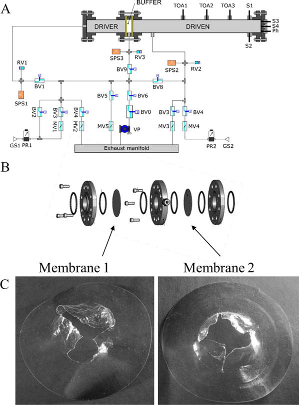
A) Schematic layout of the Shock tube with the following components: S: Transient pressure sensor, TOA: Time of arrival sensor, Ph: Photonics sensor, BV: Bellow sealed valve, GS: Gas supply, MV: Metering valve, RV: Relief valve, SPS: Static pressure sensor, VP: Vacuum pump, PR: Pressure regulator. B) exploded diagram of the dual diaphragm of the buffer region C) Burst diaphragm show uneven burst for the first stage (left panel) and a four-petal burst pattern (right panel)

A FBG is a narrow band optical filter fabricated photochemically by modifying the local structure of the silica to create a periodic variation in the local refractive index that acts like a Bragg grating. The Bragg resonance wavelength is given by

$${\lambda }_B=2n_e\Lambda$$ (5)

where λ_B is the Bragg wavelength, n_e is the effective refractive index, and Λ is the grating period. Changes in the physical strain and surrounding temperature on the FBG influence the Bragg wavelength by causing linear expansion of the material and/or changing the fiber’s refractive index. Existing literature indicates that FBG shows a temperature dependent wavelength shift of 10 pm/°C. Temperature dependence is given by equation 6.

$$\frac{\delta \lambda }{\delta t}=2\mathrm{\Lambda }\left(\frac{\delta n_e}{\delta t}\right)+2n_e\left(\frac{\delta \mathrm{\Lambda }}{\delta t}\right)$$ (6)

Since the thermo-optic coefficient is 10 times greater than thermal expansion, the wavelength shift due to temperature could be approximated as arising solely due to thermo-optic effect. The total length of FBG sensor (L = N*Λ, where N is the number of periods) along with refractive index contrast and mode confinement factor determines the grating strength (reflectivity). Nominally, the manufacturer quoted the FBG sensor as being approximately 5 mm long. The strain response for silica optical fiber is widely reported to be 1.35 nm/N which describes the wavelength shift per unit force.[23–25]

2.1 Methods: Shock tube

To characterize sensors for dynamic measurement of pressure, we developed a dual diaphragm shock tube based on the design of Stotz et. al. [26] Our shock tube is fabricated from 316 stainless steel and has an inner diameter of 5 cm. The driver section is 63.5 cm long and the driven section is 185.4 cm long. The buffer region is 2.16 cm long. The shock tube is illustrated in Figure 2A with an exploded diagram of the dual diaphragm system shown in Figure 2B. In contrast to the conventional shock tube design with a single diaphragm the dual diaphragm setup improves reproducibility and overall control of the initial conditions, which are critical to shock wave modeling and characterization. The buffer section located between the two diaphragms is initially set to a pressure midway between the driver (high pressure) and driven (low pressure) sections. The buffer section is then vented over the course of a few seconds, causing the driver/buffer diaphragm to burst. From the burst, a shockwave is generated that will burst the second diaphragm in a more predictable manner. As shown in Figure 2C, the first diaphragm shows an uneven burst pattern while the second diaphragm shows a classic four-petal pattern—which is desirable for reproducible shocks. A Uniform pressure profile of the shock was confirmed by measuring the pressure rise of four sensors on the driven-section end flange (data not shown). The diaphragm material was Lexan®^a sheet of 25 μm and 50 μm (1 mil and 2 mil) thickness. While the use of a single brass diaphragm in our shock tube allowed us to reach higher initial pressures then possible with 50 μm Lexan sheet, it often resulted in non-ideal shock conditions and hence was not pursued further.

Three high speed pressure sensors (PCB Model 113B26) are mounted equidistant (20 cm) from each other on the sidewall of the driven section and used as Time-Of-Arrival (TOA) sensors to calculate the shock wave speed. The distance from the buffer section to TOA1 is 117 cm. It is expected that the speed of the shock wave will attenuate as it propagates due to the viscous effect [27]. However, we see negligible attenuation of the speed at the pressure conditions utilized in this paper. An accurate measurement of M_S, M_R and temperature rise in the gas is key for accurate prediction of the peak pressures from the 1-D model. [20]

As shown in Figure 2A two pressure sensors (S1 and S2), opposite to each other on the circumference, are mounted on the sidewall 4.4 cm away from the end wall (unless noted otherwise, side wall sensors were piezo sensors procured from PCB and Kistler). These two sensors are used to measure the pressure levels of both the incident shock wave and reflected wave. Lastly, three sensors are mounted on the end flange, one in the geometric center (S4) and the other, a photonic sensor and a commercial piezo sensor (S3), ±2 cm away from the central sensor. These sensors are used to estimate the spatial averaging effect and enable measurement of the sum of the incident and reflected shock wave pressures.

The entire system is controlled via PC using a LabVIEW™ interface. The pressures of the driver, buffer, and driven sections are continuously recorded directly from their respective static pressure sensors, Mensor 6100 on the driver, OmegaDyne Inc PX309-KG5V on the buffer, and second identical Mensor 6100 on the driven. For every experimental trial, the shock tube is cleared of any debris and loaded with two diaphragms. Using the PC interface, the buffer and driver sections are simultaneously pressurized to slightly lower than the buffer’s desired pressure. The driver is then pressurized independently to its desired pressure. As the driver is pressurized, the diaphragm separating the driver and buffer sections will slowly deflect, causing the buffer’s pressure to increase during this process. The entire filling process takes 10 minutes to 15 minutes. Once the system stabilizes, isolation valves are closed and the data are acquired at two mega-samples-per-second with sixteen-bit vertical resolution on eight channels using a National Instruments NI-6366 digitizer). The buffer section is then vented, the diaphragms rupture and give rise to a shock wave. A typical pressure trace from the static pressure sensors is shown in Figure 3. Data for all eight sensors is processed simultaneously using a MATLAB program. In the present series of experiments the initial pressures of nitrogen gas in the driver range from 350 kPa to 800 kPa, while the driven remained at 100 kPa. Temperature of the surrounding air is measured using a calibrated platinum resistance thermometer (PRT) (Isotech Milli K).

Figure 3.

Static pressure sensors on each section of the shock tube illustrate gas filling methodology (panel on the left). The buffer and driver are filled simultaneously for the first 100 seconds. The driver is then filled to the desired pressure. The buffer is vented at about 412 seconds resulting in dual diaphragm rupture a few seconds later. The pressure values immediately before the rupture are used to determine the initial conditions. On the right the photograph illustrates the deflection of the Lexan membrane under pressure.

2.2 Methods: Photonic Sensor

We characterized the temporal response of fiber Bragg grating (FBG) sensors embedded in polydimethylsiloxane (PDMS) using the shock tube. FBG sensors (center wavelength ≈1550 nm) were embedded in 10:1 (wt:wt) PDMS via thermal curing. The fiber-PDMS composite was polymerized inside a metal sleeve that matches the dimensions of piezo sensors. This design enables the photonic sensors to be easily interchanged with commercial sensors. Figure 4 illustrates the photonic sensor design and the experimental interrogation setup similar to our previous work. [23, 28]

Figure 4.

Schematic of the FBG photonic pressure sensor (black) embedded in PDMS. The metal sleeve is about 2.5 cm long. Half the laser power is directed at a wavelength meter for feedback and the other half is transmitted to a circulator and FBG sensor. A detector on the output of the circulator measures the light reflected from the FBG sensor. The wavelength meter is used to stabilize the laser wavelength with typical precision of 1 MHz.

The optical sensors were installed in place of piezo sensors (at sensor 2 and center sensor locations) to enable comparison between the photonic sensors and piezo sensors. The response of the photonic sensors was measured by monitoring the reflected light intensity. For these measurements, the laser frequency was stabilized at either the side of the resonance fringe, on top of the resonance, or off-resonance. Pressure waves lead to longitudinal compression of the FBG sensors resulting in a blue shift of the resonance wavelength. The resonance’s shift towards shorter wavelength causes significant changes in reflected light intensity.

3.1 Results: Shock tube Characterization

The responses of the commercial sensors to shock waves are shown in Figure 5. All experiments were performed in nitrogen. The driven and driver sections were initially purged with nitrogen before each shock event. This step is needed to clean out any debris left in the shock tube from the ruptured membranes. In panel A of Figure 5, the driver pressure was set to 400 kPa, the driven pressure was 100 kPa, the diaphragm thickness was 25 μm. As expected the shockwave moving down the tube results in step changes in the piezo sensors voltage output (Figure 5A). For sensors S1 and S2 illustrated in panel A of Figure 5, a step change in signal is observed with a rather short initial flat voltage region due to the significantly smaller distance (8.8 cm) the shockwave must transverse to return as the reflected shockwave. Although the TOA is similar for both S1 and S2 the voltage amplitude significantly differs between them, which can likely be attributed to different calibration factors as these sensors were acquired from two different vendors. The sensors on the end wall (S3 and S4) exhibit a single large step from the simultaneous impact of the incident and reflected shock. Changing the initial pressure differential across the diaphragm results in progressively stronger shocks as evident by the increasingly shorter time interval between the TOA sensors (Figure 5B). The time of arrival sensors show large sudden steps in voltage located at equal time intervals; the initial step in voltage, signifying the arrival of the shockwave, is followed by a long flat voltage signal that eventually decays as the pressure starts to drop. The pressure drop is interrupted by the arrival of the reflected wave (Figure 5B) which results in another large voltage step. Our shock tube design and protocol allows us to achieve excellent reproducibility in setting the initial conditions for the shock which limits the variations in TOA to ≈ 0.1 % (see Figure 5C; TOA 1). Table 1 lists pressures measurements and Mach speeds for each of the 12 measurements performed. Our results indicate that in the range of initial conditions studied here, the theoretical predictions of Mach speed are well-correlated with measurements (Figure 6). This result supports the use of 1D theory to calculate shock pressure as presented in the discussion below.

Figure 5.

A) Response of different sensors to a shock shows uniform, flat response. Non-ideal behavior in the reflected behavior is observed at long time scales (t > 3500 μs). B) Sensors show higher Mach speed as the pre-shock pressure differential across the diaphragm is increased. The pressures of the driver section are listed. The driven section remained at approximately 100 kPa for all measurements. C) Three consecutive runs at 400 kPa differential pressure (Traces are from TOA 3) shows excellent reproducibility in the time of arrival and amplitude response as evidenced by the nearly flat, featureless difference spectra. D) The difference between each trial highlights the high level of reproducibility.

Table 1.

Initial Pressure Conditions and Measured Mach Speeds

Driver (kPa)a	Buffer (kPa)b	Driven (kPa)a	Mach Speed	Unc.c
346.37	123	99.63	1.268	0.009
347.77	127	99.64	1.276	0.006
348.14	131	99.81	1.276	0.006
394.91	171	100.02	1.302	0.003
395.3	171	100.14	1.303	0.006
397.39	177	100.11	1.312	0.005
690.15	240	100.29	1.439	0.002
693.15	231	100.55	1.445	0.002
694.55	234	99.61	1.460	0.004
795.23	298	99.34	1.492	0.007
796.46	286	99.3	1.487	0.002
797.84	401	99.33	1.489	0.001

^aUncertainty from device Manufacturer 0.01 % Full scale (Full scale is 10 MPa)

^bUncertainty from device Manufacturer 0.25 %

^cUncertainty is k = 1 determined from three independent simultaneous Mach speed measurements per shock event

Figure 6.

The top panel illustrates the correlation between experimentally measured incident Mach speed and calculated incident Mach speed based on initial conditions and gas composition using equation 2 and 3. The data (black x) represent each of the 12 measurements recorded. The fit line (red) has a slope and intercept of 0.9 and 0.1 respectively with a coefficient of determination or R squared of 0.99. The lower panel illustrates the percent difference between theory and experiment.

We estimate that for calculated P₂ of 1550.8 kPa the uncertainty is limited to 7.5 kPa or ≈ 0.5 % (due to the uncertainty in TOA). We observe significantly greater variations in the dynamic sensor’s amplitude (2.3 % std. dev. between 3 consecutive runs). The reflection wave at higher pressures shows signs of non-ideal behavior as evidenced by a rising pressure signal observed ≈2000 μs following the reflected shock’s arrival (Figure 5).

In order to evaluate the 1-D shock model [20] in for our system we examine the correlation between experimentally measured Mach speed and the predicted Mach speed -calculated using equation 3 with accurate knowledge the initial pressures and temperatures of the shock tube. The correlation is shown in Figure 6. The values of the initial pressures are measured on the Mensor pressure sensors just before membrane rupture (see Figure 3) and temperature is measured using a calibrated PRT.

Overall we find there is excellent agreement between the experiment and theory, the few percent differences are likely due to inadequate measurement of the initial conditions, error associated with the spatial averaging effects on the measurement, non-idealities of the system, and/or limitations of the theory. It is also expected that with the addition of the buffer section the standard 1-D model may not be adequate. Future work on using multiple types of membranes, extending the range of Mach speeds, and using spectroscopy to directly probe the resulting pressure and temperatures should aide in developing a more adequate model for the dual membrane shock tube.

Our results indicate that the incident shock wave presents the best opportunity for measuring transient shocks without interference from non-ideal flow conditions. The data illustrated in Figure 7 consists of the four different pressure ratios (see Table 1) and is the average of the three trials at each pressure. Overall, we find that peak amplitude is well correlated with incident (Figure 7a) and reflected shock wave pressure (Figure 7b). Our results suggest that incident and reflected shock waves if sufficiently separated in time could be used to examine the pressure response of dynamic sensors at two different pressure levels in a single shot.

Figure 7.

These plots show the high degree of linearity between raw output voltage and square of the Mach speed for both incident (panel A) and reflected (panel B) shocks. Each point represents an average of the three trials at each pressure. Error bars are k = 1.

3.2 Results: Photonic Sensor Characterization

We have used our shock tube to characterize the temporal response of FBG sensors embedded in PDMS. PDMS has long been a focus of the biomedical metrology community since PDMS’s mechanical properties can be tuned to match those of soft tissue. [29] In recent years, PDMS based phantoms have found use in characterization of dynamic response of soft tissue under blast conditions encountered in the battlefield. [30] The extensive literature on PDMS indicates the dynamic response is rate independent (see ref 16, 17 and refs cited within). High speed photography of PDMS membranes undergoing shock tube enabled inflation indicate the out-of-plane displacement is observed around ≈170 μs after the shock’s arrival while in-plane displacement can take up to ≈ 400 μs to manifest itself. [30]

Here we explore the temporal response of PDMS-FBG composite to evaluate the utility of such embedded sensors for use in future blood pressure phantoms. We measured the response time of FBG-PDMS composite by stabilizing the laser frequency to the blue side of the FBG fringe. The sensor was impacted head-on by a shock wave created by a 694 kPa/100 kPa differential (P₂ = 1.5508 MPa). As shown in Figure 8B, we observe an immediate increase in reflection intensity which corresponds to a blue shift in the Bragg resonance. We do not observe any evidence of a redshift (Bragg resonance redshift with temperature increase), indicating that the sensor embedded in thermally insulating PDMS is not sensitive to temperature changes.

Figure 8.

A) FBG sensors inserted in the end flange at steady atmospheric conditions B) end-mounted sensors. The response of PDMS embedded FBG shows an 11 μs delay relative to the co-located piezo sensors (initial driver and driven pressures were 400 kPa and 100 kPa, respectively). C) spectra for FBG sensor inserted in place of S2 shows a slight shift when steady state pressure in the driven section is increase from 100 kPa to 250 kPa. D) for the side mounted sensor the laser was tuned 1 nm to the blue of the Bragg resonance. The PDMS embedded sensor took an additional ≈250 μs relative to the co-located piezo sensor to reach peak amplitude.

The intensity changes in FBG-PDMS composite are time delayed relative to a co-located piezo sensor by ≈ 11 μs (Figure 8B). Similar results are observed for a photonic sensor located at the side of the shock tube. As shown in Figure 8C the Bragg resonance at 100 kPa is located at 1549.68 nm and is observed to blue shift to 1549.64 nm at 256 kPa of static pressure. We locked the frequency of the laser 1 nm away from the resonance and observed the intensity changes as the shock moves past the sensor. As shown in Figure 8D, the incident shock wave results in a strong change in reflection intensity as the Bragg resonance comes in to resonance with laser frequency with deformation taking ≈250 μs to manifest (relative to the arrival of the shock measured on a co-located piezo sensor). The observed timescale for PDMS based soft tissue phantom is in general agreement with published results[30]. We note that the observed times scales for PDMS-FBG composite are ≈60× slower than those observed by Rodriguez et. al.[31] for poly(methyl methacrylate)-FBG (PMMA-FBG) complex indicating the response of our composite is dominated by PDMS.

Our measurement indicates that PDMS FBG composite’s dynamic response, though slower than piezo sensors, is on the order of sub-millisecond suggesting photonic sensors embedded in PDMS phantom have sufficiently fast response times to enable measurement of biologically relevant pressure transients such as those arising due to blood flow or trauma. Additionally, the use of stiffer polymers such as PMMA may enable the use of photonic sensors as time of arrival sensors in transient measurements. A dual-comb-based interrogation scheme would allow for broad bandwidth interrogation of the sensors response on a microsecond time scale. [32] The photonic sensor size may be reduced to approximately 200 μm which coupled with faster rise time could drastically reduce the measurement uncertainty in the TOA and determination of Mach speed.

4.1 Conclusion

We have presented our recent progress in developing the infrastructure for traceable dynamic measurements of pressure. We have built and characterized a dual diaphragm shock tube that allows us to achieve shock amplitude reproducibility of 2.3 %. The uncertainty performance in the measurement scheme appears to be limited by time of arrival measurements which are limited by sensor size and data acquisition rate. Our preliminary experiments with photonic sensors suggest that fiber optic based sensors could be utilized to overcome such limitations in the future. Furthermore, we have used our shock tube to characterize the dynamic response of FBG-PDMS composite, a material of choice for soft tissue phantoms. Our results indicate that the PDMS embedded photonic sensors response to shock evolves over tens to hundreds of microsecond time scale, making it a useful system for studying transient pressures in soft tissue. We are currently working on a FBG-PDMS based blood pressure phantom and will report on its progress in a forthcoming manuscript.

References

- 1.Chen Y, Constantini S. Caveats for using shock tube in blast-induced traumatic brain injury research. Front Neurol. 2013;4:117. doi: 10.3389/fneur.2013.00117. [DOI] [PMC free article] [PubMed] [Google Scholar]
- 2.Duff RE. Shock-Tube Performance at Low Initial Pressure. Physics of Fluids. 1959;2:207. [Google Scholar]
- 3.Downes S, Knott A, Robinson I. Towards a shock tube method for the dynamic calibration of pressure sensors. Philos Trans A Math Phys Eng Sci. 2014;372:20130299. doi: 10.1098/rsta.2013.0299. [DOI] [PMC free article] [PubMed] [Google Scholar]
- 4.Petersen EL, Hanson RK. Nonideal effects behind reflected shock waves in a high-pressure shock tube. Shock Waves. 2001;10:405–420. [Google Scholar]
- 5.Syrimis M, Assanis DN. Knocking Cylinder Pressure Data Characteristics in a Spark-Ignition Engine. Journal of Engineering for Gas Turbines and Power. 2003;125:494–499. [Google Scholar]
- 6.Rosasco GJ, Bean VE, Hurst WS. A Proposed Dynamic Pressure and Temperature Primary Standard. Journal of Research of the National Institute of Standards and Technology. 1990;95:33–47. doi: 10.6028/jres.095.005. [DOI] [PMC free article] [PubMed] [Google Scholar]
- 7.Bean VE. Dynamic Pressure Metrology. Metrologia. 1994;30:737. [Google Scholar]
- 8.Hendricks JH, Olson DA. 1-15000 Pa Absolute mode comparisons between the NIST ultrasonic interferometer manometers and non-rotating force-balanced piston gauges. Measurement. 2010;43:664–674. [Google Scholar]
- 9.Egan PF, Stone JA, Hendricks JH, Ricker JE, Scace GE, Strouse GF. Performance of a dual Fabry-Perot cavity refractometer. Optics Letters. 2015;40:3945–3948. doi: 10.1364/OL.40.003945. [DOI] [PubMed] [Google Scholar]
- 10.Hendricks JH, Ricker JR, Chow JH, Olson DA. Effect of dissolved Nitrogen gas on the density of di-2-ethylhexyl sebacate: Working fluid of the NIST oil UIM pressure standard. NCSLI Measure J Meas Sci. 2009;4:52–59. [Google Scholar]
- 11.Miller AP, Tilford CR, Hendricks JH. A low differential-pressure primary standard for the range 1 Pa to 13 kPa. Metrologia. 2005;42:S187–S192. [Google Scholar]
- 12.Ahmed Z, Olson DA, Douglass K. Precision Spectroscopy to Enable Traceable Dynamic Measurements of Pressure. 2016 doi: 10.1364/CLEO_AT.2016.ATu1J.1. ATu1J.1.2016. [DOI] [PMC free article] [PubMed] [Google Scholar]
- 13.Douglass K, Olson DA. Towards a standard for the dynamic measurement of pressure based on laser absorption spectroscopy. Metrologia. 2016;53:S96–S106. doi: 10.1088/0026-1394/53/3/S96. [DOI] [PMC free article] [PubMed] [Google Scholar]
- 14.Zelan M, Arrhén F, Jarlemark P, Mollmyr O, Johansson H. Characterization of a fiber-optic pressure sensor in a shock tube system for dynamic calibrations. Metrologia. 2015;52:48–53. [Google Scholar]
- 15.Diniz A, Oliveira A, Vianna J, Neves F. Dynamic calibration methods for pressure sensors and development of standard devices for dynamic pressure. XVIII Imeko World Congress Metrology Rio de Janeiro, Brazil. 2006:17–22. [Google Scholar]
- 16.Matthews C, Pennecchi F, Eichstädt S, Malengo A, Esward T, Smith I, Elster C, Knott A, Arrhén F, Lakka A. Mathematical modelling to support traceable dynamic calibration of pressure sensors. Metrologia. 2014;51:326–338. [Google Scholar]
- 17.Sonderegger K, Dür M, Buthig J, Pantazis S, Jousten K. Very fast-opening UHV gate valve. Journal of Vacuum Science & Technology A: Vacuum, Surfaces, and Films. 2013;31:060601. [Google Scholar]
- 18.Sirohi J, Chopra I. Fundamental Understanding of Piezoelectric Strain Sensors. Journal of Intelligent Material Systems and Structures. 2000;11:246–257. [Google Scholar]
- 19.Berridge DC, Schneider SP. Calibration of PCB-132 Sensors in a Shock Tube. :1–14. RTO-MP-AVT-200. [Google Scholar]
- 20.Glass II, Sislian JP. Nonstationary Flows and Shock Waves. Clarendon Press; 1994. [Google Scholar]
- 21.Williams MD, Griffin BA, Reagan TN, Underbrink JR, Sheplak M. An AlN MEMS Piezoelectric Microphone for Aeroacoustic Applications. Journal of Microelectromechanical Systems. 2012;21:270–283. [Google Scholar]
- 22.Hjelmgren J. Dynamic meaurement of pressure-a literature survey. SP Swedish National Testing and Research Institute; 2002. [Google Scholar]
- 23.Ahmed Z, Filla J, Guthrie W, Quintavall J. Fiber Bragg Gratings Based Thermometry. NCSLI Measure. 2015;10:24–27. doi: 10.1080/19315775.2015.11721744. [DOI] [PMC free article] [PubMed] [Google Scholar]
- 24.Kronenberg P, Rastogi PK, Giaccari P, Limberger HG. Relative humidity sensor with optical fiber Bragg gratings. Optics Letters. 2002;27:1385–1387. doi: 10.1364/ol.27.001385. [DOI] [PubMed] [Google Scholar]
- 25.Mihailov SJ. Fiber Bragg Grating Sensors for Harsh Environments. Sensors. 2012;12:1898–1918. doi: 10.3390/s120201898. [DOI] [PMC free article] [PubMed] [Google Scholar]
- 26.Stotz I, Lamanna G, Hettrich H, Weigand B, Steelant J. Design of a double diaphragm shock tube for fluid disintegration studies. Rev Sci Instrum. 2008;79:125106. doi: 10.1063/1.3058609. [DOI] [PubMed] [Google Scholar]
- 27.Petersen Eric L, Hanson RK. Nonideal effects behind reflected shock waves.pdf. Shock Waves. 2001;10:405–420. [Google Scholar]
- 28.Liacouras PC, Grant G, Choudhry K, Strouse GF, Ahmed Z. Fiber Bragg Gratings Embedded in 3D-printed Scaffolds. NCSLI Measure J Meas Sci. 2015;10:50–52. [Google Scholar]
- 29.Nie X, Prabhu R, Chen WW, Caruthers JM, Weerasooriya T. A Kolsky Torsion Bar Technique for Characterization of Dynamic Shear Response of Soft Materials. Experimental Mechanics. 2011;51:1527–1534. [Google Scholar]
- 30.Bentil SA, Ramesh KT, Nguyen TD. A Dynamic Inflation Test for Soft Materials. Experimental Mechanics. 2016;56:759–769. [Google Scholar]
- 31.Rodriguez G, Sandberg RL, Lalone BM, Marshall BR, Grover M, Stevens G, Udd E. SPIE Sensing Technology + Applications. SPIE; 2014. High pressure sensing and dynamics using high speed fiber Bragg grating interrogation systems; p. 9. [Google Scholar]
- 32.Giorgetta FR, Coddington I, Baumann E, Swann WC, Newbury NR. Fast high-resolution spectroscopy of dynamic continuous-wave laser sources. Nature Photonics. 2010;4:853–857. [Google Scholar]