

Summary
Embryonic cell fates are defined by transcription factors that are rapidly deployed, yet attempts to visualize these factors in vivo often fail due to slow fluorescent protein maturation. Here we pioneer a protein tag, LlamaTag, which circumvents this maturation limit by binding mature fluorescent proteins, making it possible to visualize transcription factor concentration dynamics in live embryos. Implementing this approach in the fruit fly Drosophila melanogaster, we discovered stochastic bursts in the concentration of transcription factors that are correlated with bursts in transcription. We further used LlamaTags to show that the concentration of protein in a given nucleus depends heavily on transcription of that gene in neighboring nuclei; we speculate that this inter-nuclear signaling is an important mechanism for coordinating gene expression to delineate straight and sharp boundaries of gene expression. Thus, LlamaTags now make it possible to visualize the flow of information along the central dogma in live embryos.
In brief
A fluorescent protein tagging strategy reveals a role for inter-nuclear signaling and coordination of protein levels between neighboring nuclei in Drosophila embryogenesis.
INTRODUCTION
The cells of a developing embryo often make rapid decisions about their fate. For example, body segments of the zebrafish embryo are specified in <25 min, and a mature stripe of the segmentation gene even-skipped (eve) in the fruit fly Drosophila melanogaster is defined in <15 min (Bothma et al., 2014; Schroter et al., 2008). These cell-fate decisions are driven by the concentration dynamics of transcription factors. For example, the frequency of oscillation of her1 and her7 determines vertebrae number (Schroter et al., 2008), and the precise temporal progression of the expression of transcription factors in neural progenitors in flies and vertebrates dictates neural fates (Kohwi and Doe, 2013).
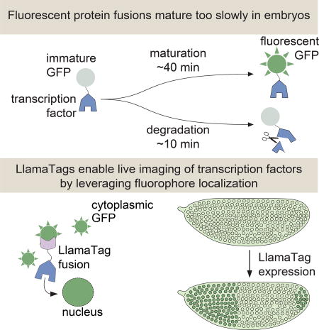
Our knowledge of how these crucial dynamics specify fate has been hampered by available technology. The widespread use of fluorescent protein fusions to transcription factors has been limited by the slow maturation step that must occur before these fusions become fluorescent. Although engineered fluorescent proteins have chromophore maturation half-times as low as 4 min in vitro or in cultured cells (Balleza et al., 2018), these half-times increase to >30 min in the embryos of model organisms such as frogs, zebrafish, worms, and flies (Dickinson et al., 2017; Hazelrigg et al., 1998; Little et al., 2011; Wacker et al., 2007). This time scale is much slower than many key processes in development. For example, the fly transcription factor Fushi Tarazu (Ftz) has a half-life of ~8 min (Edgar et al., 1987), and the Her proteins in vertebrates have half-lives of 3–20 min (Ay et al., 2013; Hirata et al., 2004). This rapid protein turnover makes visualizing the expression of these transcription factors in real time nearly impossible; the fusion protein of interest has already degraded by the time the reporter begins to fluoresce (Fig. 1A). As a result, attempts to measure transcription factor patterns in live embryos with fluorescent protein fusions have yielded undetectable or significantly delayed patterns (Drocco et al., 2011; Little et al., 2011; Ludwig et al., 2011). Thus, fluorescent protein maturation kinetics remains a major hindrance to the live imaging of cell-fate decisions during embryonic development (Fig. 1B and STAR Methods).
Figure 1. Genetically encoded LlamaTags overcome slow fluorescent protein maturation.

(A) In many model organisms such as the fly, fluorescent protein fusions are degraded much faster than the rate at which they mature and begin to fluoresce. (B) Fluorescent protein maturation masks protein concentration dynamics qualitatively and quantitatively. Total fusion protein includes molecules with both mature and non-mature GFP; the number of mature, visible fluorescent fusion proteins due to a pulse of protein production is plotted over time. Maturation and degradation rates are as in (A); see STAR Methods for model assumptions and parameters. (C, D) In the LlamaTag approach, the fluorescent protein is maternally produced, ensuring that all proteins are fluorescent and uniformly distributed throughout the embryo. Upon translation of a LlamaTagged transcription factor, the fluorescent protein binds the nanobody. Here, eGFP is translocated to the nucleus as a result of the transcription factor’s nuclear localization signal, resulting in the enrichment of nuclear fluorescence. See also Figure S1.
Here we present a novel genetically encoded tagging technique for visualizing transcription factor spatiotemporal dynamics in development by overcoming the slow kinetics of fluorescent-protein maturation. This tag is based on nanobodies, small single-domain antibodies derived from llamas (Hamers-Casterman et al., 1993), which we name LlamaTags. Our strategy employs the spatial localization of already mature fluorescent proteins as a reporter of protein concentration dynamics (Aymoz et al., 2016) rather than relying on the production of transcription factor-fluorescent protein fusions. Nanobodies are extremely versatile and present significant advantages over previous technologies for quantifying transcription factor dynamics in live embryos (see Discussion for further details). Their small size of ~15 kDa is ideal for limiting perturbations of the tagged protein’s endogenous function, and the binding of a nanobody and its target is fast (~106 M−1s−1) and of high affinity (pM-nM) (Fridy et al., 2014; Kirchhofer et al., 2010). Nanobodies have been used for a broad range of applications from stabilizing protein structure to targeting proteins to a particular subcellular location (for a thorough review of these applications, see Bieli et al. (2016) and references therein).
We established the simplicity of tagging and the wide array of measurements enabled by LlamaTags by using the development of the fruit fly as a case study. Further, by combining LlamaTags with the MS2 aptamer system for in vivo tagging of nascent mRNA (Larson et al., 2009), we simultaneously visualized transcription factor concentration and transcription. Thus, LlamaTags are a versatile tool to quantify how developmental programs are deployed in real time, at the single-cell level, in live embryos.
RESULTS
LlamaTags capture the endogenous concentration dynamics of transcription factors in development
In order to visualize the endogenous concentration dynamics of a transcription factor of interest, we fuse the transcription factor to a nanobody raised against enhanced green fluorescent protein (eGFP), and express it under the transcription factor’s endogenous regulatory sequence in conjunction with maternally deposited eGFP – ensuring ample time for eGFP maturation before the gene is expressed. When the transcription factor-nanobody fusion is translated, it binds cytoplasmic eGFP on the time scale of seconds and increases the fluorescence of bound eGFP by 1.5 fold (Fig. 1C, see below, STAR Methods, and Kirchhofer et al. (2010)). As the LlamaTagged transcription factor is imported into the nucleus to perform its regulatory function, the eGFP is imported too (Figs. 1C and 1D). Expression of the LlamaTagged protein leads to an increase in nuclear fluorescence that constitutes a direct readout of the instantaneous transcription factor concentration in each nucleus.
To ensure that mature eGFP was present in the early fly embryo before the gene of interest is expressed, we employed a transgene that expresses eGFP in developing oocytes; female flies containing this construct deposit eGFP mRNA in their eggs and, upon fertilization, this mRNA is translated into protein (Gregor et al., 2008). The eGFP rapidly diffuses, matures, and yields uniform fluorescence throughout the embryo by nuclear cycle 14 (nc14). Although LlamaTags cannot differentiate between mature and immature eGFP, this system ensures that all eGFP is mature when the genes that define the adult body plan are expressed (Jaeger et al., 2004) (Figs. 2A and S1A). eGFP does not contain a nuclear localization signal and, in the absence of a LlamaTag, shows only weak nuclear enrichment (Figs. 2A and S1B), thus providing an ideal framework for imaging nuclearly localized LlamaTagged transcription factors.
Figure 2. LlamaTags capture endogenous protein dynamics in the early embryo.

(A) In the absence of a LlamaTagged transcription factor, eGFP is uniformly distributed throughout the embryo. (B) CRISPR-mediated fusion of hb to a LlamaTag. (C,D) Hb-LlamaTag expression patterns recapitulate previous measurements obtained using fluorescent antibody staining: the early step-like Hb pattern (8 min into nc14) later forms two stripes of high protein concentration at 43 min into nc14, one in the middle of the embryo and one in its posterior. (E) Hb-LlamaTag eGFP signal per nucleus scales linearly with Hb fluorescence obtained by immunostaining. Data are normalized by their means. Error bars represent standard error over pixels within each nucleus. Inset, images of a fixed embryo in the GFP and anti-Hb channels that were used in generating the graph. See STAR Methods for further details. (F) Simultaneous visualization of Hb and Twi in an embryo initiating gastrulation using LlamaTags specific to eGFP and mCherry, respectively. Sharp edges on anterior and posterior of embryo are due to the embryo being larger than the field of view. All embryos are oriented with anterior to the left and ventral on the bottom. All scale bars are 50 µm. D, images taken from FlyEx database, see Pisarev et al. (2009). See also Figure S1–S4 and Movie S1.
To test the ability of LlamaTags to report on transcription factor dynamics, we tagged the Hunchback (Hb) protein at its endogenous locus in the Drosophila genome using CRISPR-mediated homologous recombination (Fig. 2B, see Table S1 for primer sequences) (Gratz et al., 2015). Hb is expressed in the anterior half of the early embryo, where it plays a critical role in specifying the fly body plan (Margolis et al., 1995; Perry et al., 2012). Imaging live embryos that contained both eGFP and the LlamaTagged hb locus using laser-scanning confocal microscopy revealed a pattern of bright fluorescent nuclei (Fig. 2C and Movie S1) that appeared virtually identical to the endogenous Hb pattern previously visualized in fixed embryos at different stages of development using immunohistochemistry (Fig. 2D, images taken from FlyEx database, see Pisarev et al. (2009)). The Hb-LlamaTag pattern was initially restricted to the anterior half of the embryo, and then later developed a strong stripe of expression midway along the body axis, as well as a posterior stripe characteristic of the endogenous Hb pattern. Quantification of Hb levels revealed that Hb protein concentration increases by >5× during nc14 (Fig. S4A). The Hb-LlamaTag fusion was functionally equivalent to the endogenous protein: flies homozygous for the hb-LlamaTag chromosome rescued to adulthood, even in the presence of maternally provided eGFP.
To determine whether LlamaTags accurately report protein concentration dynamics, we fixed embryos homozygous for the LlamaTagged hb locus and maternally provided fluorescent eGFP. After fixation, we fluorescently labeled Hb in these embryos in a separate channel using immunohistochemistry. Formaldehyde fixation rapidly halts any binding and unbinding of eGFP to the LlamaTag such that the fixed embryo represents an instantaneous snapshot of Hb-LlamaTag dynamics. We quantified both the nuclear intensity of eGFP and the Hb concentration as reported by immunofluorescence. The eGFP signal reporting the LlamaTag concentration was linearly related to the anti-Hb signal (Fig. 2E), providing concrete evidence that the nuclear eGFP intensity in live embryos is a direct and quantitative readout of the amount of tagged protein present at any given moment.
The linearity between the eGFP and anti-Hb signals (Fig. 2E) also suggests that the rapid binding kinetics of nanobodies in vitro is preserved in our in vivo LlamaTag system. In the STAR Methods, we show that if the binding between eGFP and the LlamaTag were slow relative to the dynamics of the Hb protein pattern, then a non-linear relation would appear in Figure 2E. The linear fit in Figure 2E also reveals an offset in the LlamaTag signal with respect to immunostaining (non-zero y-intercept). We associate this offset with excess, unbound eGFP molecules in the nucleus. In STAR Methods, we discuss a strategy for determining this offset, which we subtract from all data shown below. Taken together, these measurements demonstrate the ability of LlamaTags to faithfully report on endogenous transcription factor dynamics in development.
Next, we sought to expand the color palette to enable multicolor imaging for the simultaneous quantification of multiple transcription factors. We designed an mCherryLlamaTag using a nanobody that binds the mCherry fluorescent protein with high affinity and specificity (Fridy et al., 2014). Specifically, we fused the mCherryLlamaTag to the endogenous Twist (Twi) protein using CRISPR-mediated homologous recombination. We simultaneously imaged the endogenous Twist and Hunchback patterns by examining embryos containing maternally supplied eGFP and mCherry in addition to the Hb-eGFPLlamaTag and Twi-mCherryLlamaTag loci (Fig. 2F). The patterns of each transcription factor in their corresponding channels were consistent with previous observations (Ip et al., 1992), suggesting that both LlamaTags are completely orthogonal and do not cross-react (Fig. S4). Nuclei expressing Hb in regions of the embryo where no Twi expression is expected had no nuclear enrichment of mCherry. Similarly, nuclei in the Twi expression domain, but outside the Hb domain, displayed no nuclear enrichment of eGFP. These results demonstrate the versatility of the LlamaTag system to visualize multiple proteins simultaneously.
We sought to determine whether this approach is suitable for imaging transcription factors at later development stages, once cellularization has occurred and cells move below the embryo surface. In addition to Hb’s role in setting up the body axis of the embryo, this protein also patterns the nervous system by specifying the fate of neural progenitor cells (neuroblasts) as well as the neurons and glia that these progenitors give rise to (Kohwi and Doe, 2013).
Figure 3A shows the ventrolateral surface of a stage 9 embryo that contains maternal eGFP, LlamaTagged Hb, and has its histones marked with red fluorescent protein (RFP). Beneath this outer layer of cells, we observed cells that were morphologically distinct from those above (Fig. 3B). From their enlarged nuclear morphology and grid-like arrangement (Doe, 1992), we identified them as neuroblasts. As expected (Kohwi and Doe, 2013), Hb was expressed in a subset of these neuroblasts (high levels of nuclear eGFP, Fig. 3B). We followed the rapid changes in Hb expression in the developing nervous system over several hours (Movie S2).
Figure 3. Visualizing rapid transcription factor dynamics in the specification of neural progenitor cells.

(A) Surface of the ventolateral region of a living stage 9 embryo, homozygous for Hb-LlamaTag and containing maternally deposited eGFP and His-RFP. Anterior is to the top of the image. (B) Interior of an embryo staged as in (A), z-section 15–17 µm below the surface. The large cells are neuroblasts; a subset shows high levels of nuclear eGFP due to Hb-LlamaTag expression. Mesoderm cells that lack Hb appear in the middle of the image. (C,D) Time course of neuroblast formation from a proneural cluster of ectoderm cells. Four of the cells in the cluster have been annotated. Hb protein levels rapidly change in each cell during specification. (E) Quantification of eGFP fluorescence in the proneural cluster in C and D. (F) Z-sections of the proneural cluster after the neuroblast has descended and the ectodermal cells associated with it have started to divide. Error bars are standard deviation of quantified eGFP fluorescence from 3 quantification trials for a single proneural cluster (STAR Methods). A, B, scale bars are 15 µm; C, D, and F, snapshots are 28 µm by 28 µm. See also Figure S5 and Movie S2.
In contrast to the well-understood process of neuroblast formation, the specification of the cells each neuroblast gives rise to is still an active area of research in many model organisms (Kohwi and Doe, 2013). This identity is dictated by the sequential expression of a series of transcription factors, including Hb, in the neuroblast (Kohwi and Doe, 2013). Using LlamaTags, we determined that cells in the proneural cluster outlined in Figure 3A all initially expressed Hb at low levels (Fig 3C–F). Over 10 min, the cells upregulated Hb to varying degrees, with one cell expressing high levels of Hb while the others in the proneural cluster downregulated Hb. This “winner” changed its morphology and dived into the embryo interior to become a neuroblast (Fig 3F). Minutes later, the neuroblast underwent its first asymmetric division to generate a ganglion mother cell (Fig. S5A–B and Kohwi and Doe (2013)). We also measured LlamaTagged Hb in the nuclei of a subset of terminally differentiated neurons in the deepest layers of the nerve cord 13 h after fertilization (Fig. S5C–D). Thus, LlamaTags make it possible to observe tight temporal coupling between transcription factor dynamics and fate specification in cells within deep tissues over long time scales.
Revealing protein production and degradation dynamics at the single-cell level
After confirming that LlamaTags accurately report the concentration dynamics of transcription factor patterns in live Drosophila embryos, we turned our attention to Ftz, a transcription factor that is key to body plan segmentation (Edgar et al., 1987). Earlier work in fixed samples showed that Ftz expression is highly dynamic—the protein initially occurs in a broad pattern throughout the embryo that refines to seven sharply delineated stripes in <20 min (FlyEx database, see Pisarev et al. (2009)). Ftz mRNA and protein both have short half-lives of ~8 min, which is believed to underpin the transient nature of this pattern (Edgar et al., 1987; Edgar et al., 1986).
We fused our LlamaTag to the C-terminus of a ftz mini-gene that recapitulates endogenous Ftz expression in the early embryo (Hiromi et al., 1985). Imaging of embryos containing this transgene and maternal eGFP revealed the first real-time analysis of Ftz concentration changing in space and time in a live embryo (Fig. 4A, Movie S3). At the beginning of nc14, Ftz was present uniformly throughout the embryo. As development progressed, this pattern refined into the characteristic seven well-defined stripes (Fig. 4A). Extraction of the Ftz concentration dynamics in single nuclei revealed that, in the regions of the embryo that will ultimately contain Ftz stripes, the rate of protein synthesis exceeds that of degradation, leading to a sustained increase in Ftz levels (Fig. 4B). However, in nuclei outside the stripes, Ftz production ceased and rapid degradation led to undetectable amounts of protein (Fig. 4C). This interplay between synthesis and degradation of transcription factors has been speculated to shape the gene-expression patterns that drive the developmental regulatory network in the early fly embryo (Jaeger et al., 2004).
Figure 4. Capturing fast protein production and degradation dynamics using LlamaTags.

(A) Single-embryo, real-time protein expression dynamics of Ftz-LlamaTag. Time is measured with respect to the start of nc14. The field of view is smaller than the embryo, leading to cropping of the images. The embryo is oriented with anterior to the left and ventral on the bottom. The scale bar is 25 µm. (B) Ftz concentration in a nucleus inside a stripe as a function of time suggests the presence of protein bursts. (C) Ftz concentration in a nucleus outside a stripe as a function of time reveals Ftz degradation. Inset, exponential decay fit to Ftz degradation. Averaging fitting results for 58 nuclei yield a half-life of 7.9± 0.9 min. Error bars are standard error of the intensity values within a nucleus. See STAR Methods for further details. See also Movie S3.
We used our nuclear concentration data to extract the in vivo degradation rate of LlamaTagged Ftz; our analyses of signal decay in nuclei outside the stripes were consistent with Ftz degradation as a single exponential with a decay constant of 7.9 ± 0.9 min (Fig. 4C, inset). This measurement is comparable to reported values obtained in bulk from fixed embryos (Edgar et al., 1987), showing that LlamaTags can be used to extract in vivo transcription factor degradation rates in real time at the single-cell level in embryos.
Close examination of Ftz concentration dynamics in individual nuclei revealed that the concentration of nuclear protein does not change monotonically (Figs. 4B and 4C). Instead, the Ftz signal is punctuated by rapid, burst-like fluctuations in concentration. We hypothesized that these “protein bursts” stem primarily from stochastic bursts in transcriptional activity, which were previously reported in the context of development (Bothma et al., 2014; Fukaya et al., 2016). We therefore sought to simultaneously image Ftz protein concentration and ftz transcription in order to relate these periods of intermittent protein accumulation with transcriptional bursts. We introduced MS2 loops (Bothma et al., 2014) into the intron of our LlamaTagged ftz mini-gene (Fig. 5A). As shown in Figure 2F, the nanobody in this LlamaTag does not bind mCherry (Fridy et al., 2014; Kirchhofer et al., 2010), enabling the simultaneous visualization of ftz transcription with an mCherry-MCP fusion (Garcia et al., 2013) and LlamaTagged Ftz with eGFP. The mCherry-MCP transgene is under the control of a maternal promoter that ensures ubiquitous, fully fluorescent mCherry-MCP in the embryo by the time MCP is captured by the MS2 loops in ftz. As expected, transcription of ftz preceded the appearance of the protein pattern (Fig. 5B and Movie S4), with bursts of ftz transcription in individual nuclei immediately before transient protein bursts (Fig. 5C). In addition to correlating stochastic bursts in mRNA production with transient protein bursts, these data also constitute the first direct visualization of the transcription and protein production of a single gene in a live embryo. In contrast to Ftz, no protein bursts were observed for Hb. We attribute this lack of protein bursts to the fact that hb does not display transcriptional bursts (Bothma et al., 2014; Garcia et al., 2013).
Figure 5. Revealing the correlations among transcriptional bursts, protein bursts, and inter-nuclear coupling.

(A) Transcription of ftz and Ftz protein production are monitored by labeling the nascent mRNA using MS2 loops and the protein using a LlamaTag, and imaged using laser-scanning confocal microscopy. (B) Representative frames from a movie of ftz transcription (red) and Ftz protein concentration (green). The embryo is oriented with anterior to the left and ventral on the bottom. Time stamps indicate the time since the beginning of nc14. Scale bars are 25 µm. (C) MS2 and LlamaTag data for a nucleus within a stripe reveal the relation between transcriptional bursts and protein bursts. (D) False-colored representation of the MCP-mCherry channel for a subset of nuclei. The central nucleus does not transcribe ftz (false-colored in purple, quantification in (E)) but is surrounded by nuclei that actively transcribe the ftz transgene (false-colored in pink, quantification in (E)). The scale bar is 5 µm. (E) The center nucleus in (D) presents no detectable ftz transcription (purple line), but does show an increase and decrease in the amount of nuclear protein present (green line). The appearance of Ftz protein in the nucleus that is not transcribing ftz is related to the fact that its neighboring nuclei are actively transcribing ftz (protein levels of neighboring nuclei are shown in Fig. S6). The red line shows the sum of the traces of transcriptional activity of all of the surrounding nuclei. (F) Proposed mechanism for the sharing of mRNA and protein between nuclei through diffusion in the Drosophila syncytium. Error bars for transcriptional activity are estimated from the uncertainty in quantifying the fluorescence background. Error bars for protein concentration are standard error of the intensity values within a nucleus. See Methods for further details. See also Movie S4 and Figure S6.
Surprisingly, in a small subset of nuclei (5 out of 553), we also observed Ftz protein in the absence of transcription (Figs. 5D and 5E). Although these nuclei did not exhibit ftz transcription, their neighboring nuclei did (Fig. 5D). The combined transcriptional activity of these neighboring nuclei was consistent with the increase in protein concentration in this non-transcriptionally active nucleus (Fig. 5E). This coupling between transcription and protein concentration in neighboring nuclei provides evidence of inter-nuclear communication in the fly syncytium, where protein in one nucleus can originate from mRNA transcribed in adjacent nuclei (Fig. 5F).
Coupling between neighboring nuclei dictates protein expression patterns
The coupling measured between nuclei in Ftz is presumably mediated by the diffusion of mRNA, protein, or both through the syncytium of the early embryo. In this scenario, a transcription factor transcribed in a nucleus could dictate transcription in nearby nuclei, providing a rapid inter-nuclear signaling mechanism and shaping gene expression patterns over long length scales.
To determine whether nuclear coupling contributes to the establishment of cellular fates, we turned our attention to the transcription factor Snail (Sna). Sna (Slug/Sna2 in vertebrates) is a major determinant of epithelial-mesenchyme transitions in animal development and is stably expressed in a large and well-defined domain in the most ventral part of the embryo (Ip et al., 1992). We engineered a sna transgene containing an intron with MS2 stem loops and a fusion to the LlamaTag (Fig. 6A), allowing the observation of transcription and protein production (Fig. 6B).
Figure 6. Consequences of inter-nuclear coupling for pattern formation of Sna.

(A) Schematic of the mini-gene engineered to visualize transcription of sna with MS2 and Sna protein with the LlamaTag. (B) Visualization of sna transcription dynamics and protein production shows the progressive refinement of the Sna protein pattern. (C) Dynamics of sna transcription and protein production in nuclei 1 and 2 as indicated in B. (D) Nucleus-to-nucleus coupling strength as a function of time defined as the ratio between protein levels in transcriptionally inactive nuclei and neighboring active nuclei. (E) Schematic of the “kick start” model whereby a cell that does not transcribe sna initially can have transcription auto-activated through the diffusion of Sna from multiple neighbors. (F) mRNA and protein trace of a border nucleus in (B) that has initiated transcription as a result of Sna protein provided by neighbors. (G) False-colored nuclei showing the location and temporal change in the sna transcription boundary. B, G, scale bars are 10 µm. See also Movie S5 and Figure S7.
Live imaging of sna expression dynamics identified a subset of nuclei that did not show signs of sna transcription, but contained Sna protein due to their location next to actively transcribing nuclei (Fig. 6C). For example, protein levels in the non-transcribing nucleus 2 increased despite this nucleus being transcriptionally inactive for sna. The increase in protein presumably stems from molecules diffusing from the vicinity of transcriptionally active nuclei such as nucleus 1. Toward the end of nc14, the Sna concentration in nucleus 2 decayed while protein concentration in nucleus 1 continued to increase (Fig. 6C). We speculate that this protein decay is due to a reduction in the diffusive coupling between nuclei 1 and 2 caused by cellularization of the embryo syncytium combined with the degradation of protein in nucleus 2.
In order to measure the degree of inter-nuclear coupling in this system, we identified nuclei that showed no transcription, but that were next to nuclei that expressed sna (Fig. 6D). These measurements revealed a strong degree of coupling between neighboring nuclei early in the nuclear cycle, with the Sna concentration in a non-transcribing nucleus being roughly half the average concentration of neighbors that actively express sna (Fig. 6D). Our results suggest that approximately half of the protein in a given nucleus originates from transcripts produced by its nearest neighbors, while the remaining protein comes from its own transcription.
Sna expression is initially activated by the broad gradients of the transcription factors Dorsal and Twi (Ip et al., 1992) but, toward the second half of nc14, Sna activates its own expression (Lagha et al., 2013). Given this autoactivation, we hypothesized that strong inter-nuclear coupling contributes to shaping the Sna expression domain: Sna protein diffusing from neighboring nuclei could “kick start” transcriptionally inactive nuclei by engaging the sna positive-feedback loop (Fig. 6E). As cellularization progresses, inter-nuclear coupling ceases (Fig. 6D), effectively locking each cell into its final fate.
Our hypothesis is supported by data from nuclei that formed the final border of the Sna domain (Fig. 6F). Here, we show a representative example of a nucleus that displays no snail transcription initially, but that is surrounded by two or more nuclei that do transcribe. As the Sna concentration increases due to transcripts produced in transcriptionally active neighbors, sna transcription is “kick started” and maintained for the rest of nc14 (Fig. 6F). Uncovering this nuclear coupling and its consequences for sna activation could only have been revealed through the simultaneous live imaging of protein concentration and transcriptional activity afforded by our LlamaTag and MS2 system.
The inter-nuclear coupling revealed by our LlamaTags might have significant consequences in shaping sharp gene expression boundaries. Initially, the sna transcription boundary is ragged, with nuclei showing transcription over a range of three to four nuclear widths (Fig. 6G). However, over 30 minutes, transcriptionally inactive nuclei receive Sna protein from their active neighbors, kick starting their own transcription, and causing the boundary to transform into an almost perfectly straight line of sna expression (Fig. 6G). This new straight boundary of expression, which is essential to one of Sna’s roles in defining the architecture of the future nerve cord (Skeath and Thor, 2003), becomes stable as the coupling strength between nuclei decreases (Fig. 6D). We speculate that the “kick start” effect revealed by our live imaging may be a general mechanism for delineating straight boundaries of gene expression from initially ragged transcriptional boundaries in the fly embryo (Discussion).
Simultaneous visualization of input transcription-factor concentration and output transcription reveals the action of transcription factors at the single-cell level
To demonstrate the ability of LlamaTags to reveal the link between input transcription factor concentration and the transcription of target genes, we quantified the repression of the stripe 2 enhancer of eve by Krüppel (Kr) (Bothma et al., 2014). Eve stripe 2 is activated by Bicoid and Hb, and repressed on the posterior side of the embryo by Kr (Frasch and Levine, 1987; Small et al., 1992). We created transgenic flies containing a Kr-LlamaTag mini-gene, which contains all of the enhancers that drive Kr transcription in the early embryo (Perry et al., 2011), and monitored the output transcription of an eve stripe 2 reporter using MS2 (Bothma et al., 2014) (Fig. 7A).
Figure 7. Uncovering the dynamics of transcription-factor input and transcriptional output at the single-cell level.

(A) Strategy for LlamaTagging the Kr repressor and monitoring its regulation of eve stripe 2 transcription using MS2. (B) As time progresses, the increase in concentration of Kr-LlamaTag repressor (green) sharpens the posterior boundary of the stripe 2 of eve transcription (red). Scale bars are 25 µm. The embryo is oriented with anterior to the left and ventral on the bottom. (C,D) Input Kr concentration and output eve transcription for nuclei (C) within the stripe and (D) in the Kr repression domain reveal continuous transcriptional bursts at low Kr concentration, as well as less transcriptional bursting at high Kr concentrations. The scale bars in insets correspond to 10 µm. Error bars for transcriptional activity are estimated from the uncertainty in quantifying the fluorescence background. Error bars for protein concentration are standard error of the intensity values within a nucleus. See STAR Methods for further details. See also Movie S6.
Each nucleus in the movie of the development of an embryo (Fig. 7B and Movie S6) affords an opportunity to quantify how the changing concentration of the Kr input repressor dictates the output transcriptional activity of eve stripe 2. Nuclei within the stripe presented low but detectable Kr levels and eve transcriptional bursts throughout the nuclear cycle (Fig. 7C). In contrast, nuclei located within Kr’s domain to the posterior of the stripe underwent different transcriptional dynamics: their eve transcriptional bursts shut down completely as development progressed and the Kr concentration increased (Fig. 7D). Thus, LlamaTags make it possible to determine how the changing concentrations of input transcription factors in individual nuclei dictate output transcriptional dynamics.
DISCUSSION
By combining this fluorescent protein capture strategy with techniques to visualize transcription, we “lit up” the central dogma in development and uncovered bursts of nuclear protein concentration that are correlated with transcriptional bursts (Figs. 4, 5 and 6). The ability to correlate transcription and protein concentration dynamics over multiple nuclei made it possible to show that, in the early embryo, gene expression in neighboring nuclei is tightly coupled: transcription of a gene in one nucleus can strongly influence the concentration of protein in a neighboring nucleus, effectively providing a rapid inter-nuclear signaling mechanism.
It is well established that the diffusion of maternally deposited morphogens in the early embryo helps to define the broad spatial gradients that provide positional information for the later activation of zygotic transcription (Gregor et al., 2007b). However, until now, it has been unknown to what extent diffusion of zygotic gene products between nuclei occurs in the embryo, and how much this influences patterning. Modeling approaches have suggested that there is negligible diffusion of such zygotic gene products (Jaeger et al., 2004), while significant diffusive coupling has been invoked to explain the decrease in variability observed when comparing transcriptional activity to accumulated levels of mRNA and protein (Gregor et al., 2007a; Little et al., 2013). However, until this study, the impossibility of visualizing zygotic gene products in real time has limited our ability to determine whether coupling occurs, and how significant it is.
In addition to providing a means for passively averaging out fluctuations in transcriptional activity across cells, this strong coupling endows the early embryo with a rapid inter-nuclear signaling mechanism. When combined with regulatory motifs that include positive feedback, inter-nuclear signaling can effectively coordinate gene expression among cells that are many cell diameters away from one another and potentially specify emergent features such as the sharp and straight gene expression boundary we observed for sna. Positive feedback loops can, on their own, result in the switch-like adoption of expression levels (Davidson, 2006), but cell-cell coupling provides a mechanism for spatially coordinating expression patterns. Interestingly, like sna, eve and ftz are also initially activated in broad domains by a combination of maternal and zygotic factors, but their patterns sharpen as their positive feedback loops are activated (Jiang et al., 1991; Lagha et al., 2013; Schier and Gehring, 1992). Thus, we speculate that this “kick start” mechanism may be a general strategy for delineating straight and sharp boundaries of gene expression from initially ragged transcriptional boundaries.
Finally, using LlamaTags, we quantified the correspondence between input transcription-factor concentration and output transcriptional dynamics at the single-cell level for Kr acting on stripe 2 of eve (Fig. 7). To uncover the mechanisms at play as activators and repressors regulate transcription, it will be necessary to analyze data such as those shown in Figures 7C and 7D with yet-to-be-developed computational methods that correlate output transcriptional dynamics with the concentration dynamics of input transcription factors.
Future applications of LlamaTags
The ability to visualize the concentration dynamics of input transcription factors and to correlate this signal with output transcriptional dynamics gives us a unique opportunity to map the topology of endogenous developmental networks by monitoring their dynamics (Lipinski-Kruszka et al., 2015). For example, gene networks in bacteria were carefully mapped by imaging protein fluctuations propagating through the network (Dunlop et al., 2007). This kind of mapping reveals more than which gene is connected to which other gene: it assigns a precise mathematical meaning to each connection that is rich with mechanistic insight, can expose the precise molecular mechanisms that regulate gene expression (Munsky et al., 2012), and is a necessary first step toward building a predictive understanding of how regulatory programs define cell fates (Garcia et al., 2016).
Comparison to other tagging approaches for the visualization of transcription factors
Recently, a plethora of tagging techniques have been developed to fluorescently label proteins. For example, SunTags and Spaghetti Monster fluorescent proteins rely on the binding of stabilized antibody fragments fused to fluorescent proteins or bound to organic dyes (Tanenbaum et al., 2014; Viswanathan et al., 2015). Proteins can also be visualized through fusion to a HaloTag, which covalently binds an organic dye (Los et al., 2008).
Despite the widespread use of these approaches for studies in cell culture, the adoption of these techniques to uncover the regulatory mechanisms of embryonic development has been limited. SunTag arrays and Spaghetti Monster fluorescent proteins are large (~1,400 kDa and ~1,700 kDa, respectively), potentially altering the physical properties of the protein of interest (Tanenbaum et al., 2014; Viswanathan et al., 2015). In contrast, the LlamaTag-GFP complex adds <45 kDa to the tagged protein, and does not affect endogenous protein function (Fig. 2).
In embryos, HaloTags and some implementations of Spaghetti Monster fluorescent proteins require the introduction of organic dye through injection. Such injections into individual embryos are time consuming, can affect embryo variability and experimental reproducibility, and require a specialized injection apparatus tightly integrated with the imaging pipeline. Further, the injected dye is not uniformly distributed throughout the embryo (Crocker et al., 2017), posing a challenge to the interpretation of experimental results. On the other hand, LlamaTags are fully encoded genetically, circumventing the need for injections.
Finally, these previous approaches to fluorescently tag proteins are limited in terms of their multiplexing capabilities. SunTags utilize a specially designed single-chain variable fragment such that only one type of fluorescent protein can be employed at a time (Tanenbaum et al., 2014). HaloTags tags and Spaghetti Monster fluorescent proteins are limited by the orthogonal chemistries available for dye binding to no more than two colors (Los et al., 2008; Viswanathan et al., 2015). In contrast, as discussed below, LlamaTags can be easily extended to simultaneously visualize multiple transcription factors. Thus, while it is possible to implement previous tagging technologies to study transcription factor patterns in development, LlamaTags are a superior alternative.
Multiplex fluorescence imaging of transcription factor concentration and signaling state using LlamaTags
Most regulatory decisions in development result from the simultaneous action of multiple transcription factors. As a result, it is critical to expand the LlamaTag palette to achieve multiplexing. Importantly, nanobodies raised against a fluorescent protein do not cross-react with fluorescent proteins originating from other species (Fridy et al., 2014). We have already developed a LlamaTag specific to mCherry that, combined with the anti-GFP LlamaTag introduced in this work, allows the simultaneous visualization of two protein channels (Fig. 2F). This palette of LlamaTags can be further expanded by raising nanobodies against fluorescent proteins from different species such as yellow fluorescent protein from Phialidium (Fridy et al., 2014). Finally, this approach could be complemented by the creation of new nanobodies that recognize a specific transcription factor. This nanobody could then be fused to a fluorescent protein and expressed uniformly throughout the embryo. After translation, a transcription factor binds the nanobody-fluorescent protein fusion and transports it into the nucleus, yielding the same enrichment of nuclear fluorescence that we reported here (Fig. 1). However, since the nanobody binds a transcription factor instead of a fluorescent protein, there is complete spectral freedom for labeling. This approach can also be utilized to distinguish between phosphorylated and non-phosphorylated species of the same transcription factor, a regulatory feature that is pervasive in developmental programs (Jimenez et al., 2000).
To conclude, LlamaTags overcome a crucial limitation that has prohibited developmental biologists from following the processes of the central dogma with high spatiotemporal resolution. We envision that LlamaTags can be readily applied to a broad range of model organisms amenable to transgenic control and live imaging. The combination of these tags with techniques to label nascent mRNAs will open the door to quantifying the flow of information along regulatory networks in development writ large.
STAR Methods text
CONTACT FOR REAGENT AND RESOURCE SHARING
Further information and requests for resources and reagents should be directed to and fulfilled by the Lead Contact, Hernan Garcia (hggarcia@berkeley.edu).
EXPERIMENTAL MODEL AND SUBJECT DETAILS
The experimental model used in this study is Drosophila melanogaster. All individuals used in this study were embryos that were imaged as detailed below during the first 15 hours of development. Embryos were allowed to develop at room temperature and conditions unless otherwise stated. Embryo sex is not reported as it is not believed to influence any of the measurements reported here.
Fly Strains/Genotypes
The unpublished fly lines that were used in this study were generated by incorporating engineered transgenes into the genome of the yw fly strain, or by altering endogenous loci of the yw strain using CRISPR-Cas9 mediated homologous recombination. The Cloning and Transgenesis section details how each transgene was generated and genomically integrated, as well as how specific loci in the genome were edited using CRISPR-Cas9 mediated homologous recombination.
Hunchback and Twist
To image the expression of Hb protein in the early embryo we performed fly crosses to combine the integrated transgene that encodes maternal eGFP (Bcd>eGFP-STOP) with the modified chromosome that contained the LlamaTaged Hb locus (Hb-LlamaTag). Both the male and female parents of the embryos that were imaged had the following genotype, yw; Bcd>eGFP-STOP; Hb-LlamaTag. This ensured that the embryos that were imaged were homozygous for the Hb-LlamaTag gene and also contained maternally derived eGFP. In order to image both Hb protein and Twi protein simultaneously we performed fly crosses to arrive at a maternal fly line that contained transgenes that drove maternal eGFP (Bcd>eGFP-STOP), maternal mCherry (Bcd>mCherry-STOP) and also the Hb-LlamaTag (here we will refer to it as Hb-eGFPLlamaTag to differentiate it from the mCherryLlamaTag). The full genotype of these mothers was yw; Bcd>eGFP-STOP/Bcd>mCherry-STOP; Hb-eGFPLlamaTag. These were then crossed with male flies that were homozygous for the Twist locus that had been tagged with the mCherry LlamaTag (yw;Twi-mCherryLlamaTag;+). This ensured that the embryos that were imaged contained maternally deposited eGFP, mCherry and had one copy of both the tagged Hb and Twi loci.
In order to image Hb protein at later stages of development we used fly crosses to incorporate a published histone RFP transgene (yw; His2av-RFP; +, (Garcia et al., 2013)) into the line we imaged. Female flies were made that had the following genotype, yw; His2av-RFP/Bcd>eGFP-STOP; Hb-LlamaTag, and crossed to males that were of the following genotype, yw; +; Hb-LlamaTag, in order to generate embryos that contained ubiquitously expressed eGFP, histones marked with RFP and the tagged Hb locus.
Fushi tarazu, Snail and Kruppel
To image the ftz transgene that was tagged with the LlamaTag we took females of the genotype yw;+;Bcd>eGFP-STOP, and crossed them to males that were homozygous for the modified ftz transgene, yw; +; Ftz-LlamaTag. In order to visualize both transcription and protein we generated a recombinant chromosome that contained both ubiquitous eGFP and also mCherry-MCP and used fly crosses to generate a stable line of the following genotype: yw; +; Bcd>eGFP-STOP, nanos>NLS-mCherry-MCP. Females of this line were then crossed with males that were of the following genotypes, yw; +; Ftz-MS2-LlamaTag, and yw; +; Sna-MS2-LlamaTag to simultaneously image transcription and protein production for the ftz and sna transgenes, respectively.
To image Kr protein and eve transcription simultaneously the previously published line yw; +; eve2-MS2-yellow (Bothma et al., 2014) was crossed with yw; +; Kr-LlamaTag to produce yw; +; eve2-MS2-yellow, Kr-LlamaTag. Males of this genotype were then crossed with females of the following genotype, yw; +; Bcd>eGFP-STOP, nanos>NLS-mCherry-MCP, and the progeny from this cross were imaged.
METHOD DETAILS
Cloning and Transgenesis
Transgenes expressing eGFP, mCherry and MCP
All primers sequences used in this study can be found in Table S1. To provide mature fluorophores for LlamaTag imaging a construct driven by the maternal Bicoid (Bcd) promoter was used: the pCASPER-eGFP-STOP-Bcd and pCASPER-mCherry-STOP-Bcd constructs we created were modeled off an earlier eGFP-Bcd fusion (Gregor et al., 2008). A premature stop codon was introduced between the fluorophore and Bcd to provide maternally deposited eGFP or mCherry mRNA for the imaging of all Llama-Tagged fusion proteins. eGFP levels expressed by this fly line are characterized in Figure S1. Cloning of these P-element construct was performed using Gibson Assembly. Constructs were injected into yw embryos by BestGene.
To simultaneously image protein using LlamaTags and transcription using MS2, we created a fly line that maternally expressed a fusion protein with a nuclear localization signal (NLS-mCherry-MCP); without the NLS, MCP-mCherry was actively exported from the nuclei of early Drosophila embryos (Fukaya et al., 2016). pCASPER4-pNOS-NLS-mCherry-MCP-αTubulin 3’UTR was created through the modification of pCASPER4-pNOS-tdMCP-GFP-αTubulin 3’UTR (kindly provided by Michael Stadler), tdMCP-GFP was excised from the plasmid using NheI and SacII, replaced with SV40-mCherry-MCP through Gibson Assembly, and the resulting construct was injected into yw embryos by BestGene.
Transgenes with LlamaTags andMS2 repeats
Drosophila codon-optimized nanobodies against eGFP (Enhancer clone from Kirchhofer et al. (2010)) and mCherry (LaM-2 clone from Fridy et al. (2014)) were ordered from IDT as gBlocks and used as templates. Sequences with the appropriate overhangs for cloning were generated via PCR. Details of the creation of the Kruppel (Kr), Fushi Tarazu (Ftz), and Snail (Sna) eGFPLlamaTag fusions appear with the sequence data. Briefly, the 3’ fusions of Ftz, Sna, and Kr utilizing poly-glycine linkers were based on previously published mini-genes (Hiromi et al., 1985; Perry et al., 2011) and inserted into a pBPhi backbone (Bothma et al., 2014) using Gibson Assembly. To create the Ftz minigene with both MS2 and the eGFPLlamaTag a unique AgeI cut site was introduced to the ftz intron of the Ftz-LlamaTag mini gene and stable MS2 loops (Bothma et al., 2014) were added through blunt end ligation. Since sna lacks an intron, MS2 loops were placed at the 5’ end of the sna gene through Gibson Assembly and were flanked by hb intron sequence to prevent any possible interference in translational efficiency. MS2 loops were digested from pCR4-24xMS2sl (Addgene plasmid #31865) with BamHI + BglII. Kr, Ftz, and Sna constructs were integrated on chromosome 3 using Bloomington strain 9750 and injections were performed by Rainbow Transgenic Flies.
Creation ofLlamaTaged loci using CRISPR-Cas9
Both constructs for CRISPR-Cas9 mediated homologous recombination to produce Hb-eGFPLlamaTag and Twi-mCherryLlamaTag were constructed similarly to the Kr and Ftz mini-genes using Gibson Assembly and the gRNAs were selected using the FlyCRISPR website; see sequence repository for further details (Gratz et al., 2015). Transformants harboring the Hb-LlamaTag construct were identified by crossing injected males with females expressing ubiquitous eGFP; embryos were fluorescently screened for the Hb pattern and then raised to establish Hb-LlamaTag lines. Injections were performed by BestGene into strain 54591. A 3×P3 driven dsRed cassette was added to the 3’ end of the Twi construct for visual screening of CRISPR transformants (Gratz et al., 2015).
Embryo preparation for live imaging
Embryos were dechorinated using bleach, mounted between a semipermeable membrane (Biofolie, In Vitro Systems & Services) and a coverslip (1.5, 18 mm × 18 mm), and embedded in Halocarbon 27 oil (Sigma). Flattening of the embryos makes it possible to image a larger number of nuclei in the same focal plane without significantly impacting early development processes (Garcia et al., 2013). In order to image the developing nervous system, embryos were dechorinated and then immersed in Halocarbon oil to enable staging by eye. Based on their morphology, embryos were selected such that they had just undergone the rapid phase of germband elongation, and were then mounted with their ventral surface facing the coverslip as described above. These embryos were then imaged through developmental stages 9 to 11. To image the ventral nerve cord in late embryos overnight collections of embryos towards the end of stage 15 were staged by morphology, and then mounted ventrally as described above.
Immunohistochemical staining
Immunostaining was performed as reported in Lagha et al. (2013). Briefly, nuclei were stained using DAPI and Hb was labelled using a rabbit anti-Hb primary antibody in conjunction with an Alexa 555 donkey anti-rabbit secondary. The Hunchback antibody was a gift from Nipam Patel.
Laser scanning confocal microscopy
Embryos for all figures with the exception of Figure S1 were imaged using a Zeiss LSM 780 confocal microscope. Confocal imaging on the Zeiss was performed using a Plan-Apochromat 40×/1.4NA oil immersion objective. GFP and MCP-mCherry were excited with a laser wavelength of 488 nm (35 µW laser power) and 561 nm (20 µW laser power), respectively. Fluorescence was detected using the Zeiss QUASAR detection unit. For low magnification movies, sequential Z-stacks were acquired consisting of 12 planes separated by 1 µm with the detector gain set to 714.26 V, pixel size 0.692 µm, pinhole size 114.54 µm with a 14.2 µs pixel dwell time (no line or frame averaging was used). For high magnification movies, sequential Z-stacks were acquired consisting of 13 to 23 planes (number of z planes were increased during the progression of nc14 in order to accommodate the lengthening of nuclei) separated by 0.5 µm with the detector gain set to 777.92 V, pixel size 0.208 µm, pinhole size 107.12 µm with a 6.3 µs pixel dwell time (no line or frame averaging was used).
Data for Figure S1 was obtained using a Leica SP8 laser scanning confocal with a White Light Laser, a HC PL APO CS2 63×/1.40 OIL objective, and a pinhole size of 2 AU at 488 nm. Pixel size was 0.426 µm, excitation frequencies were 488 nm (5 µW laser power) and 589 nm. Z-stacks consisting of 9 planes separated by 1 µm were acquired using the microscope’s HyD in photon counting mode.
Model relating fluorescence to protein level
To determine how the fluorescence reported by a regular fluorescent protein fusion is related to the total protein concentration, we model fluorescent protein production, maturation, and degradation using rate equations. Protein maturation and degradation occur according to first-order kinetics such that the dynamics of the production of proteins that are fluorescent, [ProteinFluo], and those that have not yet matured, [ProteinDark], are given by
| (1) |
| (2) |
| (3) |
Here, r(t) is the protein production rate, which may be time dependent, λ is the protein degradation rate, and γ is the rate at which the fluorescent protein matures. If we assume that, initially, no protein is present such that [Protein](t = 0) = 0, these rate equations can be solved in the frequency domain by taking their Laplace transforms. Taking the Laplace transform of Equation and 1 and 2 and re-arranging yields
| (4) |
| (5) |
| (6) |
Here, s is the complex Laplace variable and X(s), Y(s), and R(s) are the Laplace transforms of ProteinDark(t), ProteinFluo(t) and r(t), respectively. The following two identities related to inverting Laplace transforms allows us to readily convert Equations 4 to 6 back into the time domain:
| (7) |
| (8) |
Here, ℒ−1{}, denotes the inverse Laplace transform, and, F(s) and G(s) are the Laplace transforms of the time domain functions f(t) and g(t), respectively. Using Equations 7 and 8, we can transform Equation 6 to the time domain,
| (9) |
| (10) |
| (11) |
We can similarly transform Equation 5 to the time domain to obtain,
| (12) |
| (13) |
All of the variables in the integrand of Equation 13 are strictly positive, which implies that the second term in this equation is always negative. Thus, the actual amount of fluorescence observed is always less than what would be observed if all the fluorescent proteins had matured. These equations can be solved numerically for various forms of r(t); Figure 1 in the main text contains a particular realization of the solution where we assume a Gaussian pulse of protein production ( , where A = 20, σ = 1.5 min, τp = 5 min, protein half-life is 10 min (λ = 0.069 min−1), and the maturation half-life is 40 min (γ = 0.017 min−1). These half-lives are typical for the early fly embryo (Edgar et al., 1987; Little et al., 2011). As shown Figure 1 in the main text, the small fraction of mature fluorescent proteins leads to significantly less signal than would be observed were all proteins to mature instantaneously.
Consequence of fluorescent protein maturation delay
To gain further intuition about this system, we derive closed form expressions for the delay between the fluorescent signal and the actual protein concentration, and for the reduction in the observed signal shown in Figure 1. To obtain these solutions we solve for Equation 13 and Equation 11 assuming that there is a sharp pulse of protein synthesis at a time τp, i.e. r(t) = δ(t − τp) where δ(t) is a Dirac delta function. Thus,
| (12) |
| (13) |
Figure S2 contains plots for Equations 12 and 13 that depict how the total amount of protein and fluorescence signal changes for different values of maturation half-time in time when there is a pulse of protein production at t = 0. By taking the derivative of Equation 13 and solving for when it is zero, we can determine the time at which the peak in fluorescence signal occurs, tPF, given by
| (14) |
In this case, the amount of protein peaks at time τp, and since all the variables in Equation 14 are strictly positive, tPF is always greater than τp. As a result, there is a delay between the peak in the amount of protein and the peak fluorescence. When the protein half-life is much smaller than the fluorophore maturation half-life (λ ≫ γ), this expression can be further simplified and approximated by
| (15) |
which shows that, to first order, the time for maximum fluorescence signal scales inversely with the protein degradation rate. The full expression for the time at which fluorescence peaks, shown in Equation 14, can be substituted into Equation 13 in order to calculate the maximum fluorescence value. The peak in the total protein is obtained by evaluating Equation 12 at t = τp. The ratio of these two values is taken to determine a correction factor, CorFluo, that, when applied to the measured peak fluorescence, yields the actual amount of protein present
| (14) |
| (15) |
This expression alone is not particularly illuminating, but by substituting in different values for γ and λ, obtain a clear idea for how significant the difference is between the measured fluorescence and the actual amount of protein is in various kinetic regimes. For example, when the rate of fluorescence maturation is equal to the protein half-life, γ = λ, the correction factor that needs to be applied to the measured florescence is significant (CorFluo = 4). In the fly embryo the proteins have half-lives on the order of 10 minutes and maturation half-lives on the order of 40 minutes. Substituting the corresponding rates into Equation 15 yields a correction factor of more than an order of magnitude at CorFluo = 12.
Interpretation of the LlamaTag fluorescence signal
In the previous section, we showed that protein concentration is not accurately captured by fluorescent protein fusions due to slow fluorophore maturation. The rapid association kinetics between LlamaTags and mature fluorescent proteins make it possible to overcome this limitation. When a LlamaTagged transcription factor is localized to a nucleus, this binding causes a rapid increase in nuclear fluorescence with respect to the nuclear eGFP level in the absence of LlamaTag (Fig. S1). The absolute nuclear fluorescence, FluoN, is the sum of two terms: the concentration of free GFP, [GFP], and the concentration of transcription factor that is complexed to GFP, [Protein ◦ GFP],
| (16) |
In order to relate the measured fluorescence to the number of LlamaTagged transcription factors present in the nucleus, we need to account for the presence of unbound GFP. In the following subsection we show that, indeed, nuclear fluorescence in our LlamaTag construct can be easily related to the protein concentration when the nanobody-GFP interaction kinetics are faster than the time scales of protein production and degradation.
Rapid binding results in a linear relationship between fluorescence and protein concentration
By exploring the behavior of the rate equations that describe the binding of GFP to the LlamaTagged protein, we can determine how the total amount of protein is related to the measured nuclear fluorescence. The rate equations that describe the kinetics of the key molecular species, in a particular nucleus, are given by
| (17) |
| (18) |
| (19) |
Here, [Protein] is the nuclear concentration of protein that has been LlamaTagged, [GFP] is the concentration of the unbound GFP, and [Protein ◦ GFP] is the concentration of transcription factor that is bound to GFP through the LlamaTag. r(t) is the rate at which protein is produced, λ is rate of protein degradation, ka is the association rate between GFP and the LlamaTag, and kd is the rate at which GFP and the LlamaTag dissociate. [GFP0] is the concentration of GFP in the nucleus in the absence of any LlamaTagged protein, Ve is the embryo volume, and Vn is the volume of a nucleus. Note that these equations do not account for the diffusion of GFP between nuclei. Since GFP diffuses rapidly within the early fly embryo (D = 24 µm2/s) (Abu-Arish et al., 2010), we expect GFP to quickly move between neighboring nuclei, which have a typical separation of 6 µm.(Gregor et al., 2007b) As a result, we assume that there is fast mixing of GFP throughout the embryo and that there is a negligible spatial modulation of the concentration of free GFP.
Equation 19 states that there is a constant amount of GFP present in the embryo. Vn[Protein ◦ GFP] is the total amount of protein-bound GFP present in the nucleus, while Ve[GFP] is the total amount of unbound GFP throughout the whole embryo. The sum of these two quantities is equal to Ve[GFP0], the absolute amount of GFP delivered by the fly mother. By rearranging the equation, we obtain
| (20) |
which makes it possible to relate the bound and unbound GFP concentrations. Note that a Drosophila egg is Ve ≈ 10−2mm3, (Markow et al., 2009) while single nucleus is Vn ≈ 10−8mm3. Thus, such that [GFP] ≈ [GFP0], the concentration of unbound GFP is largely unaffected by the bound fraction.
These rate equations can be solved numerically, using estimates for the different parameters from the literature. Using previous measurements of the nuclear concentration of GFP expressed off of the bicoid promoter (Gregor et al., 2008) and an absolute calibration of GFP fluorescence in the embryo (Abu-Arish et al., 2010; Gregor et al., 2007a; Xu et al., 2015) yield values of [GFP0] ≈ 100 nM. In vitro measurements of binding kinetics result in ka ≈ 106 M−1s−1 and kd ≈ 10−3 s−1 (Fridy et al., 2014).
Figure S3A shows how the nuclear fluorescence and protein concentration compare to one another for the parameters stated above. As shown in the figure, the nuclear fluorescence is offset from the actual protein concentration due to the unbound GFP, but closely tracks the protein concentration. Indeed, Figure S3B predicts that nuclear fluorescence and nuclear protein concentration are linearly related. This prediction is in agreement with our experimental observations presented for the Hb profile in Figure 2D, lending support to the claim that the nuclear fluorescence signal from the LlamaTag is a faithful reporter of protein concentration. Experimentally, the offset in the fluorescence signal is obtained by measuring the fluorescence of nuclei lacking the protein. This offset fluorescence value is then subtracted from our nucleus of interest in order to obtain a signal that is proportional to the nuclear LlamaTag concentration.
The results shown in Figure S3 stem from assuming that the measured in vitro values for the GFP-nanobody interaction apply to the in vivo setting. In Figure S4 we explore how the measured fluorescence is related to the protein concentration if the association kinetics was orders of magnitude slower than the values reported in vitro. As shown in Figure S4A, even though the nuclear fluorescence qualitatively captures the protein concentration dynamics, Figure S4B now shows that the simple linear relationship between the two magnitudes breaks down. As a result, if our experimental system was in this parameter regime, the results shown in Figure 2D would dramatically deviate from a line.
Extended model to allow ~ for nuclear enrichment of GFP
We begin by considering a simplified case where a transcription factor fused to nanobody is only present in the nucleus. We will assume that all binding reactions equilibrate on a time scale much faster than any nuclear import and export rate for both the GFP and transcription factors. The equations describing the concentration equilibrium of the different species are
| (1) |
and
| (2) |
where GFPC and GFPN are the cytoplasmic and nuclear concentrations of free GFP, respectively, and KG = GFPC/GFPN the corresponding dissociation constant for equilibrium between the cytoplasmic and nuclear populations. The nuclear concentration of free transcription factor-nanobody fusion is TFN, while GFP − TFN is the concentration of the transcription factor-nanobody-GFP complex in the nucleus.
In the absence of transcription factor, the cytoplasmic (FluoC) and nuclear (FluoN) fluorescence levels, are equal to GFPC and GFPN, respectively. As a result, the dissociation constant KG can be calculated by measuring the quantity
| (3) |
In the presence of nanobody-tagged transcription factor, the nuclear fluorescence will be given by
| (4) |
We can use Equation 3 to rewrite Equation 4 as
| (5) |
Since, in this simplified model, the transcription factor can only be found in the nucleus, we know that FluoC = GFPC. As a result, the amount of transcription factor bound to GFP is given by
| (6) |
and thus can be obtained by subtracting the rescaled cytoplasmic fluorescence from the nuclear fluorescence signal.
Ultimately, we are interested in the total concentration of nuclear transcription factor, TFtot,N and not just the concentration of the transcription factor-GFP complex. These quantities are related through the dissociation constant, Kd, defined by Equation 2 such that
| (7) |
This equation can be rewritten as
| (8) |
which, using TFtot,N = TFN + GFP − TFN, leads to
| (9) |
As a result, we see that, if Kd ≪ GFPN, then all transcription factors will be bound by GFP, resulting in TFtot = GFP − TFN. Thus, assuming that GFPtot,N ~ GFPN which we discuss further below, Kd ≪ GFPN such that the nuclear transcription factor concentration can be measured from
| (10) |
Modeling cytoplasmic transcription factor
The previous model did not explicitly take into account cytoplasmic transcription factor. Here, we extend the previous model to account for the cytoplasmic concentration of transcription factor-nanobody fusion, TFC, and of the complex with GFP, GFP − TFC. Building on Equations 1 and 2, this system is described by
| (11) |
| (12) |
| (13) |
| (14) |
and
| (15) |
Here, we have assumed that the equilibrium between the cytoplasmic and nuclear fraction of both complexed and non-complexed transcription factor is given by KTF.
Once again, the nuclear fluorescence is given by
| (16) |
In addition, we now need to account for the cytoplasmic fluorescence
| (17) |
We now invoke the definitions of the dissociation constants for free GFP and TF complex transport, and , respectively in order to rewrite the cytoplasmic fluorescence as
| (18) |
We rewrite this equation as
| (17) |
which can be plugged into Equation 16 to express the nuclear fluorescence as
| (18) |
We then arrive at the expression describing the concentration of transcription factor-GFP complex in terms of the nuclear and cytoplasmic fluorescence values given by
| (19) |
Finally, under the condition GFPtot,N ≫ TFtot,N such that GFPtot,N ≈ GFPN, we get
| (19) |
This equation tells us that the only difference between the simple model in the previous, and this more complex model accounting for the presence of transcription factor in the cytoplasm is the factor . If the transcription factor import and export remain unchanged during development, then KTF remains constant such that FluoN − KGFluoC is proportional to the total transcription factor concentration in the nucleus, TFtot,N.
QUANTIFICATION AND STATISTICAL ANALYSIS
The statistical details of experiments can be found in the related figure legends and Results section, and are elaborated on in more detail in the sections below.
Quantifying transcriptional activity
Transcriptional activity was quantified largely in accordance with the protocol described in Garcia et al. (2013), with differences detailed below. In order to detect nuclei, NLS-mCherry-MCP slices were maximum projected at each time point. Nuclei were segmented using an object-detection approach based on the Laplacian of Gaussian filter kernel. Nuclei were tracked during nuclear cycles. Transcription spots were detected in three-dimensions and assigned to their closest nucleus. Following Garcia et al. (2013), we use Z-sections that are small and oversample in z, and set our imaging range to go both above and below the nuclei such that transcription foci are always maintained in focus. When multiple spots were detected in the vicinity of a nucleus, only the brightest one was kept.
To determine spot intensity, an estimate of the local fluorescent background was produced for each particle: a 2D Gaussian fit to the peak plane of each spot was used to determine the offset, which was used as background estimator. Background as a function of time was fitted to a smooth spline. The spot intensity is calculated by integrating the particle fluorescence over a circle with a radius of 6 pixels, and then subtracting the background estimated from the background spline at each time point. The standard deviation of the offset of the data around this spline is used to estimate the imaging error associated with each particle.
Quantifying live protein concentration early
The intensity in the protein channel was calculated by finding the average pixel intensity in the GFP channel of all the pixels within the nuclear mask. This was done for three z-layers (each separated by 0.5 microns), where the central layer had the highest mean fluorescence and the uncertainty was calculated as the standard error in the mean value. For each dataset the eGFP offset was determined (as described in detail in the “Interpretation of the LlamaTag fluorescence signal” subsection of Methods Details) and subtracted to yield the final protein intensity.
Quantifying Hb levels in fixed embryos
To determine whether LlamaTags accurately report protein concentration dynamics (See Figure 2E), we fixed embryos homozygous for the LlamaTagged hb locus and maternally provided fluorescent eGFP. After fixation, we fluorescently labeled Hb in these embryos by using a rabbit anti-Hb primary antibody in conjunction with an Alexa 555 donkey anti-rabbit secondary, and identified nuclei using DAPI. We quantified both the total nuclear intensity of eGFP and the Hb concentration as reported by immunofluorescence using the same approach we used for live imaging as described in the previous paragraph, with the difference being that the signal in the DAPI channel was used to define the nuclear mask.
The embryo shown Figure 2E was used to generate the corresponding plot of nuclear intensity of eGFP and the Hb concentration. For this plot the nuclear intensity of eGFP and the Hb concentration was quantified for 889 nuclei. This data fit well to a straight line with an offset (coefficient of variation of 0.9675), as determined by linear regression using a least squares approach. This same approach was conducted for 3 other embryos with 899, 850 and 876 nuclei which yielded coefficient of variation values again close to one of 0.9540, 0.9748 and 0.9669.
Ftz protein dynamics
To determine the half-life of the Ftz protein, concentration profiles of 58 nuclei, drawn from 3 different embryos were used. These specific 58 concentration profiles were chosen because they contained long periods where the Ftz protein concentration was monotonically decreasing, which allowed us to accurately determine the protein’s half-life. Non-linear regression using a least squares approach to a single decaying exponential was used to determine the protein half-life for individual profiles and then these values were averaged to yield a mean half-life value of 7.9 ± 0.9 min, where the uncertainty was calculated as the standard error in the mean.
Measuring Hb levels late
To calculate the GFP intensity in the ectodermal cells of the nervous system, a different approach had to be adopted because there are many morphologically complex cells over a range of depths. In order to measure nuclear GFP intensity in these cells, a manual approach was adopted whereby at every time point the cell of interest was identified by eye and the z layer where the nucleus was largest was chosen to perform quantification on. The GFP intensity inside the nucleus was estimated by summing over a manually chosen circular region of radius 5 pixels and then averaging the GFP signal in this region. This process was performed for every cell of interest for all time points, and repeated 3 times per cell to get an average value for the GFP signal. The standard deviation of these measurements was used to estimate the error.
Calculating Coupling Strength
In order to calculate the degree of coupling across the Snail boundary the following analysis was performed. By examining the time traces of all the nuclei, it was possible to determine which subset of nuclei showed no signs of transcription, but had neighbors that did transcribe. For every nucleus in the set, we then calculated the average amount of protein in each neighbor that showed protein levels above background. We then took the ratio of the protein amount in the cell that did not show signs of transcription and the average amount of snail protein in neighbors that did show active transcription. This process was repeated for the 11, 9 and 13 border nuclei of 3 different embryos, the mean in this value calculated, and the standard error was used to estimate the error in the mean.
DATA AND SOFTWARE AVAILABILITY
All plasmid sequences from this study can be downloaded from https://benchling.com/garcialab/f_/I4DUzneS-llamatagvectors-public.
Supplementary Material
(A) In the absence of LlamaTagged proteins, the cytoplasmic eGFP levels are uniform throughout the embryo. This fluorescence does not change during nc14. Error bars are the standard deviation across pixels. (B) Cytoplasmic-to-nuclear eGFP fluorescence ratio in the absence of LlamaTag obtained throughout the embryo over nuclear cycles 12 to 14. The mean ratio is . Error bar is standard deviation over pixels.
Live embryos homozygous for Hb-LlamaTag, containing maternally deposited eGFP, and expressing a His-RFP transgene. (A) Dynamics of ganglion mother cell specification by neuroblasts. Here, we focus on two neuroblasts that have just delaminated: NB1 expresses Hb, while NB2 does not (0 min). Shortly after delaminating, NB1 and NB2 enter mitosis and divide (5 min). This division leads to a new neuroblast, and to ganglion mother cells GMC1 and GMC2 (13 min). These cells position themselves below their mother neuroblasts. Note that only NB1, which expressed Hb, produces the Hb-positive ganglion mother cell GMC1. (B) Downregulation of Hb expression in neuroblasts as they divide to give rise to ganglion mother cells. NB1 has just delaminated, whereas NB2 has undergone a division and produced a GMC. Hb is downregulated in NB2 with respect to the levels in NB1, which is consistent with the progression of the neuroblast in the temporal specification series (Grosskortenhaus et al., 2005). NB3 does not express Hb and is included as a reference for basal eGFP level. (C) Confocal stack of the ventral nerve cord of a stage 15 Drosophila embryo. The stack starts at the ectoderm of the embryo, and moves deeper to show the nerve cord. In the most dorsal parts of the nerve cord (the deepest part) we see segmentally repeated patterns of neurons that have an enrichment of eGFP in their nuclei. In addition, the characteristic “ladder” structure where the axon bundles are found is visible. (D) Zoomed-in view of a single segment of the nerve cord showing that a specific subset of neurons presents Hb expression in their nuclei, consistent with previous results (Grosskortenhaus et al., 2005). All scale bars are 10 µm.
Ftz protein production during nc 14 for 7 neighboring nuclei are monitored by labeling protein using a LlamaTag, and imaged using laser-scanning confocal microscopy. The scale bar is 5 µm.
False-colored nuclei showing the sna transcription boundary and also which nuclei did not show any sign of transcription during the observation period. The scale bar is 10 µm.
Spatiotemporal evolution of the Hb protein expression pattern during the course of nc14. The sharp edges seen in the image are the result of the embryo being larger than the field of view. Movie is 340 µm × 161 µm.
Ventrolateral region of a living stage 9 embryo, homozygous for Hb-LlamaTag, and containing maternally deposited eGFP and His-RFP. The different panels show different depths of the embryo in order to be able to see the cell movements and changes in Hb expression levels as the cells change fate and divide. Each panel is 143 µm × 91 µm.
Spatiotemporal evolution of the Ftz protein expression pattern during the course of the second half of nc14. The sharp edges seen in the image are the result of the embryo being larger than the field of view. Movie is 510 µm × 267 µm.
Spatiotemporal evolution of ftz transcription (red puncta) and Ftz protein (green) expression patterns during the course of nc14. The sharp edges seen in the image are the result of part of the embryo being out of the field of view. Movie is 531 µm × 233 µm.
Embryo with ventral side down and a LlamaTagged Snail gene. Notice the refinement of the boundary of the Snail pattern and then subsequent invagination of the cells that express snail. Movie is 353 µm × 162 µm.
Spatiotemporal evolution of the Kr protein expression pattern (green) and eve stripe 2 mRNA expression pattern (red puncta) during the course of nc14. Movie is 151 µm × 151 µm.
This table contains the sequences of all the primers that were used during the course of this study.
Simulation results for a protein production temporal profile described by a Gaussian pulse given by (A = 100, σ = 3 min and τp = 5 min, protein half-life is ln(2)/λ=10 min, ka = 2×10⁶ M−1s−1 and kd = 10−3 s−1). (A) The nuclear fluorescence signal presents an offset with respect the actual protein concentration due to the unbound GFP, but otherwise tracks actual protein concentration dynamics. (B) Nuclear fluorescence as a function of protein concentration for the simulation in (A) clearly shows a linear relationship between the two magnitudes.
Simulation results for a protein production temporal profile described by a Gaussian as in Figure S2 (A = 100, σ = 3 min and τp = 5 min, protein half-life is ln(2)/λ=10 min, ka = 2×10⁴ M−1s−1 and kd = 10−3 s−1). (A) When the association rate is slowed by several orders of magnitude relative to the one used in Figure S2, the nuclear fluorescence no longer tracks the protein concentration. (B) The relationship between the amount of GFP-bound protein and total protein is distorted because of hysteresis: younger protein molecules are less likely to have GFP bound than older ones.
(A) Hb-LlamaTag fluorescence as a function of anterior-posterior position along the embryo and time into nc14. eGFP fluorescence in nuclei along the dorsal side of the embryo were quantified and the background signal (shown in plot) subtracted away. The error bars represent the standard deviation in the mean fluorescence calculated over multiple nuclei per anterior-posterior position. (B) Simultaneous visualization of Hb and Twi in embryo starting to undergo gastrulation using LlamaTags specific to eGFP and mCherry, respectively. Sharp edges on anterior and posterior of embryo are due to the embryo being larger than the field of view. The eGFP and mCherry channels have been separated to clearly reveal the lack of cross talk between the two LlamaTags: in nuclei that are dorsal and anterior, where there are high levels of Hb, but no Twi, no nuclear enrichment of mCherry was detected. Similarly, in nuclei that are ventral and posterior, where there are high levels of Twi, but no Hb, no nuclear enrichment of eGFP was measured.
A novel protein tagging strategy for imaging transcription factor dynamics in live embryos
Discovery of dynamic bursts in the concentration of transcription factors
Observation of strong inter-nuclear coupling of gene expression in fly embryos
Coupling provides a rapid signaling mechanism that can shape gene expression patterns
Acknowledgments
We thank Rob Phillips for extensive discussions and advice throughout this work, and for help in writing this manuscript, and Nipam Patel for his invaluable discussion regarding the neuroblast work. We also thank Nathan Belliveau, Paul Blainey, Xavier Darzacq, Yang Joon Kim, Nicholas Lammers, Sean Medin, David Savage, Allyson Sgro and members of the Garcia lab for useful discussions on the manuscript, and Michael Stadler for sharing unpublished reagents. This work was supported by the Burroughs Wellcome Fund Career Award at the Scientific Interface, the Sloan Research Foundation, the Human Frontiers Science Program, the Searle Scholars Program, the Shurl & Kay Curci Foundation, the NIH Director’s New Innovator Award (DP2 OD024541-01), and an NSF CAREER Award (1652236) to H.G.G.
Footnotes
Publisher's Disclaimer: This is a PDF file of an unedited manuscript that has been accepted for publication. As a service to our customers we are providing this early version of the manuscript. The manuscript will undergo copyediting, typesetting, and review of the resulting proof before it is published in its final citable form. Please note that during the production process errors may be discovered which could affect the content, and all legal disclaimers that apply to the journal pertain.
Author Contributions
Conceptualization, J.P.B. and H.G.G.; Methodology J.P.B., M.R.N. and H.G.G.; Investigation J.P.B. and M.R.N.; Writing, J.P.B, M.R.N and H.G.G; Funding Acquisition, H.G.G.; Resources, S.A.; Supervision, J.P.B and H.G.G.
Declaration of Interests
The authors declare no competing interests.
References
- Abu-Arish A, Porcher A, Czerwonka A, Dostatni N, Fradin C. High mobility of bicoid captured by fluorescence correlation spectroscopy: implication for the rapid establishment of its gradient. Biophys J. 2010;99:L33–35. doi: 10.1016/j.bpj.2010.05.031. [DOI] [PMC free article] [PubMed] [Google Scholar]
- Ay A, Knierer S, Sperlea A, Holland J, Ozbudak EM. Short-lived Her proteins drive robust synchronized oscillations in the zebrafish segmentation clock. Development. 2013;140:3244–3253. doi: 10.1242/dev.093278. [DOI] [PubMed] [Google Scholar]
- Aymoz D, Wosika V, Durandau E, Pelet S. Real-time quantification of protein expression at the single-cell level via dynamic protein synthesis translocation reporters. Nature communications. 2016;7:11304. doi: 10.1038/ncomms11304. [DOI] [PMC free article] [PubMed] [Google Scholar]
- Balleza E, Kim JM, Cluzel P. Systematic characterization of maturation time of fluorescent proteins in living cells. Nat Methods. 2018;15:47–51. doi: 10.1038/nmeth.4509. [DOI] [PMC free article] [PubMed] [Google Scholar]
- Bieli D, Alborelli I, Harmansa S, Matsuda S, Caussinus E, Affolter M. Development and Application of Functionalized Protein Binders in Multicellular Organisms. Int Rev Cell Mol Biol. 2016;325:181–213. doi: 10.1016/bs.ircmb.2016.02.006. [DOI] [PubMed] [Google Scholar]
- Bothma JP, Garcia HG, Esposito E, Schlissel G, Gregor T, Levine M. Dynamic regulation of eve stripe 2 expression reveals transcriptional bursts in living Drosophila embryos. Proc Natl Acad Sci U S A. 2014;111:10598–10603. doi: 10.1073/pnas.1410022111. [DOI] [PMC free article] [PubMed] [Google Scholar]
- Crocker J, Tsai A, Muthusamy AK, Lavis LD, Singer RH, Stern DL. Nuclear Microenvironments Modulate Transcription From Low-Affinity Enhancers. bioRxiv. 2017 doi: 10.7554/eLife.28975. [DOI] [PMC free article] [PubMed] [Google Scholar]
- Davidson EH. The regulatory genome : gene regulatory networks in development and evolution. Burlington, MA; San Diego: Academic; 2006. [Google Scholar]
- Dickinson DJ, Schwager F, Pintard L, Gotta M, Goldstein B. A Single-Cell Biochemistry Approach Reveals PAR Complex Dynamics during Cell Polarization. Developmental cell. 2017;42:416–434. e411. doi: 10.1016/j.devcel.2017.07.024. [DOI] [PMC free article] [PubMed] [Google Scholar]
- Doe CQ. Molecular markers for identified neuroblasts and ganglion mother cells in the Drosophila central nervous system. Development. 1992;116:855–863. doi: 10.1242/dev.116.4.855. [DOI] [PubMed] [Google Scholar]
- Drocco JA, Grimm O, Tank DW, Wieschaus E. Measurement and perturbation of morphogen lifetime: effects on gradient shape. Biophys J. 2011;101:1807–1815. doi: 10.1016/j.bpj.2011.07.025. [DOI] [PMC free article] [PubMed] [Google Scholar]
- Dunlop MJ, Cox RS, III, Levine JH, Murray RM, Elowitz MB. Regulatory activity revealed by dynamic correlations in gene expression noise. Nature Genetics. 2007;40:1493–1498. doi: 10.1038/ng.281. [DOI] [PMC free article] [PubMed] [Google Scholar]
- Edgar BA, Odell GM, Schubiger G. Cytoarchitecture and the patterning of fushi tarazu expression in the Drosophila blastoderm. Genes Dev. 1987;1:1226–1237. doi: 10.1101/gad.1.10.1226. [DOI] [PubMed] [Google Scholar]
- Edgar BA, Weir MP, Schubiger G, Kornberg T. Repression and turnover pattern fushi tarazu RNA in the early Drosophila embryo. Cell. 1986;47:747–754. doi: 10.1016/0092-8674(86)90517-9. [DOI] [PubMed] [Google Scholar]
- Frasch M, Levine M. Complementary patterns of even-skipped and fushi tarazu expression involve their differential regulation by a common set of segmentation genes in Drosophila. Genes Dev. 1987;1:981–995. doi: 10.1101/gad.1.9.981. [DOI] [PubMed] [Google Scholar]
- Fridy PC, Li Y, Keegan S, Thompson MK, Nudelman I, Scheid JF, Oeffinger M, Nussenzweig MC, Fenyo D, Chait BT, et al. A robust pipeline for rapid production of versatile nanobody repertoires. Nat Methods. 2014;11:1253–1260. doi: 10.1038/nmeth.3170. [DOI] [PMC free article] [PubMed] [Google Scholar]
- Fukaya T, Lim B, Levine M. Enhancer Control of Transcriptional Bursting. Cell. 2016 doi: 10.1016/j.cell.2016.05.025. [DOI] [PMC free article] [PubMed] [Google Scholar]
- Garcia HG, Brewster RC, Phillips R. Using synthetic biology to make cells tomorrow's test tubes. Integr Biol (Camb) 2016;8:431–450. doi: 10.1039/c6ib00006a. [DOI] [PMC free article] [PubMed] [Google Scholar]
- Garcia HG, Tikhonov M, Lin A, Gregor T. Quantitative imaging of transcription in living Drosophila embryos links polymerase activity to patterning. Curr Biol. 2013;23:2140–2145. doi: 10.1016/j.cub.2013.08.054. [DOI] [PMC free article] [PubMed] [Google Scholar]
- Gratz SJ, Rubinstein CD, Harrison MM, Wildonger J, O'Connor-Giles KM. CRISPR-Cas9 Genome Editing in Drosophila. Curr Protoc Mol Biol. 2015;111:31, 32, 31–20. doi: 10.1002/0471142727.mb3102s111. [DOI] [PMC free article] [PubMed] [Google Scholar]
- Gregor T, McGregor AP, Wieschaus EF. Shape and function of the Bicoid morphogen gradient in dipteran species with different sized embryos. Dev Biol. 2008;316:350–358. doi: 10.1016/j.ydbio.2008.01.039. [DOI] [PMC free article] [PubMed] [Google Scholar]
- Gregor T, Tank DW, Wieschaus EF, Bialek W. Probing the limits to positional information. Cell. 2007a;130:153–164. doi: 10.1016/j.cell.2007.05.025. [DOI] [PMC free article] [PubMed] [Google Scholar]
- Gregor T, Wieschaus EF, McGregor AP, Bialek W, Tank DW. Stability and nuclear dynamics of the bicoid morphogen gradient. Cell. 2007b;130:141–152. doi: 10.1016/j.cell.2007.05.026. [DOI] [PMC free article] [PubMed] [Google Scholar]
- Grosskortenhaus R, Pearson BJ, Marusich A, Doe CQ. Regulation of temporal identity transitions in Drosophila neuroblasts. Developmental cell. 2005;8:193–202. doi: 10.1016/j.devcel.2004.11.019. [DOI] [PubMed] [Google Scholar]
- Hamers-Casterman C, Atarhouch T, Muyldermans S, Robinson G, Hamers C, Songa EB, Bendahman N, Hamers R. Naturally occurring antibodies devoid of light chains. Nature. 1993;363:446–448. doi: 10.1038/363446a0. [DOI] [PubMed] [Google Scholar]
- Hazelrigg T, Liu N, Hong Y, Wang S. GFP expression in Drosophila tissues: time requirements for formation of a fluorescent product. Dev Biol. 1998;199:245–249. doi: 10.1006/dbio.1998.8922. [DOI] [PubMed] [Google Scholar]
- Hirata H, Bessho Y, Kokubu H, Masamizu Y, Yamada S, Lewis J, Kageyama R. Instability of Hes7 protein is crucial for the somite segmentation clock. Nat Genet. 2004;36:750–754. doi: 10.1038/ng1372. [DOI] [PubMed] [Google Scholar]
- Hiromi Y, Kuroiwa A, Gehring WJ. Control elements of the Drosophila segmentation gene fushi tarazu. Cell. 1985;43:603–613. doi: 10.1016/0092-8674(85)90232-6. [DOI] [PubMed] [Google Scholar]
- Ip YT, Park RE, Kosman D, Yazdanbakhsh K, Levine M. dorsal-twist interactions establish snail expression in the presumptive mesoderm of the Drosophila embryo. Genes Dev. 1992;6:1518–1530. doi: 10.1101/gad.6.8.1518. [DOI] [PubMed] [Google Scholar]
- Jaeger J, Surkova S, Blagov M, Janssens H, Kosman D, Kozlov KN, Manu, Myasnikova E, Vanario-Alonso CE, Samsonova M, et al. Dynamic control of positional information in the early Drosophila embryo. Nature. 2004;430:368–371. doi: 10.1038/nature02678. [DOI] [PubMed] [Google Scholar]
- Jiang J, Hoey T, Levine M. Autoregulation of a segmentation gene in Drosophila: combinatorial interaction of the even-skipped homeo box protein with a distal enhancer element. Genes Dev. 1991;5:265–277. doi: 10.1101/gad.5.2.265. [DOI] [PubMed] [Google Scholar]
- Jimenez G, Guichet A, Ephrussi A, Casanova J. Relief of gene repression by torso RTK signaling: role of capicua in Drosophila terminal and dorsoventral patterning. Genes Dev. 2000;14:224–231. [PMC free article] [PubMed] [Google Scholar]
- Kirchhofer A, Helma J, Schmidthals K, Frauer C, Cui S, Karcher A, Pellis M, Muyldermans S, Casas-Delucchi CS, Cardoso MC, et al. Modulation of protein properties in living cells using nanobodies. Nature structural & molecular biology. 2010;17:133–138. doi: 10.1038/nsmb.1727. [DOI] [PubMed] [Google Scholar]
- Kohwi M, Doe CQ. Temporal fate specification and neural progenitor competence during development. Nat Rev Neurosci. 2013;14:823–838. doi: 10.1038/nrn3618. [DOI] [PMC free article] [PubMed] [Google Scholar]
- Lagha M, Bothma JP, Esposito E, Ng S, Stefanik L, Tsui C, Johnston J, Chen K, Gilmour DS, Zeitlinger J, et al. Paused Pol II Coordinates Tissue Morphogenesis in the Drosophila Embryo. Cell. 2013;153:976–987. doi: 10.1016/j.cell.2013.04.045. [DOI] [PMC free article] [PubMed] [Google Scholar]
- Larson DR, Singer RH, Zenklusen D. A single molecule view of gene expression. Trends Cell Biol. 2009;19:630–637. doi: 10.1016/j.tcb.2009.08.008. [DOI] [PMC free article] [PubMed] [Google Scholar]
- Lipinski-Kruszka J, Stewart-Ornstein J, Chevalier MW, El-Samad H. Using dynamic noise propagation to infer causal regulatory relationships in biochemical networks. ACS Synth Biol. 2015;4:258–264. doi: 10.1021/sb5000059. [DOI] [PMC free article] [PubMed] [Google Scholar]
- Little SC, Tikhonov M, Gregor T. Precise developmental gene expression arises from globally stochastic transcriptional activity. Cell. 2013;154:789–800. doi: 10.1016/j.cell.2013.07.025. [DOI] [PMC free article] [PubMed] [Google Scholar]
- Little SC, Tkacik G, Kneeland TB, Wieschaus EF, Gregor T. The formation of the Bicoid morphogen gradient requires protein movement from anteriorly localized mRNA. PLoS Biol. 2011;9:e1000596. doi: 10.1371/journal.pbio.1000596. [DOI] [PMC free article] [PubMed] [Google Scholar]
- Los GV, Encell LP, McDougall MG, Hartzell DD, Karassina N, Zimprich C, Wood MG, Learish R, Ohana RF, Urh M, et al. HaloTag: a novel protein labeling technology for cell imaging and protein analysis. ACS Chem Biol. 2008;3:373–382. doi: 10.1021/cb800025k. [DOI] [PubMed] [Google Scholar]
- Ludwig MZ, Manu, Kittler R, White KP, Kreitman M. Consequences of Eukaryotic Enhancer Architecture for Gene Expression Dynamics, Development, and Fitness. PLoS Genet. 2011;7:e1002364. doi: 10.1371/journal.pgen.1002364. [DOI] [PMC free article] [PubMed] [Google Scholar]
- Margolis JS, Borowsky ML, Steingrimsson E, Shim CW, Lengyel JA, Posakony JW. Posterior stripe expression of hunchback is driven from two promoters by a common enhancer element. Development. 1995;121:3067–3077. doi: 10.1242/dev.121.9.3067. [DOI] [PubMed] [Google Scholar]
- Markow TA, Beall S, Matzkin LM. Egg size, embryonic development time and ovoviviparity in Drosophila species. J Evol Biol. 2009;22:430–434. doi: 10.1111/j.1420-9101.2008.01649.x. [DOI] [PubMed] [Google Scholar]
- Munsky B, Neuert G, van Oudenaarden A. Using gene expression noise to understand gene regulation. Science. 2012;336:183–187. doi: 10.1126/science.1216379. [DOI] [PMC free article] [PubMed] [Google Scholar]
- Perry MW, Boettiger AN, Levine M. Multiple enhancers ensure precision of gap gene-expression patterns in the Drosophila embryo. Proc Natl Acad Sci U S A. 2011 doi: 10.1073/pnas.1109873108. [DOI] [PMC free article] [PubMed] [Google Scholar]
- Perry MW, Bothma JP, Luu RD, Levine M. Precision of hunchback expression in the Drosophila embryo. Curr Biol. 2012;22:2247–2252. doi: 10.1016/j.cub.2012.09.051. [DOI] [PMC free article] [PubMed] [Google Scholar]
- Pisarev A, Poustelnikova E, Samsonova M, Reinitz J. FlyEx, the quantitative atlas on segmentation gene expression at cellular resolution. Nucleic Acids Res. 2009;37:D560–566. doi: 10.1093/nar/gkn717. [DOI] [PMC free article] [PubMed] [Google Scholar]
- Schier AF, Gehring WJ. Direct homeodomain-DNA interaction in the autoregulation of the fushi tarazu gene. Nature. 1992;356:804–807. doi: 10.1038/356804a0. [DOI] [PubMed] [Google Scholar]
- Schroter C, Herrgen L, Cardona A, Brouhard GJ, Feldman B, Oates AC. Dynamics of zebrafish somitogenesis. Developmental dynamics : an official publication of the American Association of Anatomists. 2008;237:545–553. doi: 10.1002/dvdy.21458. [DOI] [PubMed] [Google Scholar]
- Skeath JB, Thor S. Genetic control of Drosophila nerve cord development. Curr Opin Neurobiol. 2003;13:8–15. doi: 10.1016/s0959-4388(03)00007-2. [DOI] [PubMed] [Google Scholar]
- Small S, Blair A, Levine M. Regulation of even-skipped stripe 2 in the Drosophila embryo. EMBO J. 1992;11:4047–4057. doi: 10.1002/j.1460-2075.1992.tb05498.x. [DOI] [PMC free article] [PubMed] [Google Scholar]
- Tanenbaum ME, Gilbert LA, Qi LS, Weissman JS, Vale RD. A protein-tagging system for signal amplification in gene expression and fluorescence imaging. Cell. 2014;159:635–646. doi: 10.1016/j.cell.2014.09.039. [DOI] [PMC free article] [PubMed] [Google Scholar]
- Viswanathan S, Williams ME, Bloss EB, Stasevich TJ, Speer CM, Nern A, Pfeiffer BD, Hooks BM, Li WP, English BP, et al. High-performance probes for light and electron microscopy. Nat Methods. 2015;12:568–576. doi: 10.1038/nmeth.3365. [DOI] [PMC free article] [PubMed] [Google Scholar]
- Wacker SA, Oswald F, Wiedenmann J, Knochel W. A green to red photoconvertible protein as an analyzing tool for early vertebrate development. Developmental dynamics : an official publication of the American Association of Anatomists. 2007;236:473–480. doi: 10.1002/dvdy.20955. [DOI] [PubMed] [Google Scholar]
- Xu H, Sepulveda LA, Figard L, Sokac AM, Golding I. Combining protein and mRNA quantification to decipher transcriptional regulation. Nat Methods. 2015;12:739–742. doi: 10.1038/nmeth.3446. [DOI] [PMC free article] [PubMed] [Google Scholar]
Associated Data
This section collects any data citations, data availability statements, or supplementary materials included in this article.
Supplementary Materials
(A) In the absence of LlamaTagged proteins, the cytoplasmic eGFP levels are uniform throughout the embryo. This fluorescence does not change during nc14. Error bars are the standard deviation across pixels. (B) Cytoplasmic-to-nuclear eGFP fluorescence ratio in the absence of LlamaTag obtained throughout the embryo over nuclear cycles 12 to 14. The mean ratio is . Error bar is standard deviation over pixels.
Live embryos homozygous for Hb-LlamaTag, containing maternally deposited eGFP, and expressing a His-RFP transgene. (A) Dynamics of ganglion mother cell specification by neuroblasts. Here, we focus on two neuroblasts that have just delaminated: NB1 expresses Hb, while NB2 does not (0 min). Shortly after delaminating, NB1 and NB2 enter mitosis and divide (5 min). This division leads to a new neuroblast, and to ganglion mother cells GMC1 and GMC2 (13 min). These cells position themselves below their mother neuroblasts. Note that only NB1, which expressed Hb, produces the Hb-positive ganglion mother cell GMC1. (B) Downregulation of Hb expression in neuroblasts as they divide to give rise to ganglion mother cells. NB1 has just delaminated, whereas NB2 has undergone a division and produced a GMC. Hb is downregulated in NB2 with respect to the levels in NB1, which is consistent with the progression of the neuroblast in the temporal specification series (Grosskortenhaus et al., 2005). NB3 does not express Hb and is included as a reference for basal eGFP level. (C) Confocal stack of the ventral nerve cord of a stage 15 Drosophila embryo. The stack starts at the ectoderm of the embryo, and moves deeper to show the nerve cord. In the most dorsal parts of the nerve cord (the deepest part) we see segmentally repeated patterns of neurons that have an enrichment of eGFP in their nuclei. In addition, the characteristic “ladder” structure where the axon bundles are found is visible. (D) Zoomed-in view of a single segment of the nerve cord showing that a specific subset of neurons presents Hb expression in their nuclei, consistent with previous results (Grosskortenhaus et al., 2005). All scale bars are 10 µm.
Ftz protein production during nc 14 for 7 neighboring nuclei are monitored by labeling protein using a LlamaTag, and imaged using laser-scanning confocal microscopy. The scale bar is 5 µm.
False-colored nuclei showing the sna transcription boundary and also which nuclei did not show any sign of transcription during the observation period. The scale bar is 10 µm.
Spatiotemporal evolution of the Hb protein expression pattern during the course of nc14. The sharp edges seen in the image are the result of the embryo being larger than the field of view. Movie is 340 µm × 161 µm.
Ventrolateral region of a living stage 9 embryo, homozygous for Hb-LlamaTag, and containing maternally deposited eGFP and His-RFP. The different panels show different depths of the embryo in order to be able to see the cell movements and changes in Hb expression levels as the cells change fate and divide. Each panel is 143 µm × 91 µm.
Spatiotemporal evolution of the Ftz protein expression pattern during the course of the second half of nc14. The sharp edges seen in the image are the result of the embryo being larger than the field of view. Movie is 510 µm × 267 µm.
Spatiotemporal evolution of ftz transcription (red puncta) and Ftz protein (green) expression patterns during the course of nc14. The sharp edges seen in the image are the result of part of the embryo being out of the field of view. Movie is 531 µm × 233 µm.
Embryo with ventral side down and a LlamaTagged Snail gene. Notice the refinement of the boundary of the Snail pattern and then subsequent invagination of the cells that express snail. Movie is 353 µm × 162 µm.
Spatiotemporal evolution of the Kr protein expression pattern (green) and eve stripe 2 mRNA expression pattern (red puncta) during the course of nc14. Movie is 151 µm × 151 µm.
This table contains the sequences of all the primers that were used during the course of this study.
Simulation results for a protein production temporal profile described by a Gaussian pulse given by (A = 100, σ = 3 min and τp = 5 min, protein half-life is ln(2)/λ=10 min, ka = 2×10⁶ M−1s−1 and kd = 10−3 s−1). (A) The nuclear fluorescence signal presents an offset with respect the actual protein concentration due to the unbound GFP, but otherwise tracks actual protein concentration dynamics. (B) Nuclear fluorescence as a function of protein concentration for the simulation in (A) clearly shows a linear relationship between the two magnitudes.
Simulation results for a protein production temporal profile described by a Gaussian as in Figure S2 (A = 100, σ = 3 min and τp = 5 min, protein half-life is ln(2)/λ=10 min, ka = 2×10⁴ M−1s−1 and kd = 10−3 s−1). (A) When the association rate is slowed by several orders of magnitude relative to the one used in Figure S2, the nuclear fluorescence no longer tracks the protein concentration. (B) The relationship between the amount of GFP-bound protein and total protein is distorted because of hysteresis: younger protein molecules are less likely to have GFP bound than older ones.
(A) Hb-LlamaTag fluorescence as a function of anterior-posterior position along the embryo and time into nc14. eGFP fluorescence in nuclei along the dorsal side of the embryo were quantified and the background signal (shown in plot) subtracted away. The error bars represent the standard deviation in the mean fluorescence calculated over multiple nuclei per anterior-posterior position. (B) Simultaneous visualization of Hb and Twi in embryo starting to undergo gastrulation using LlamaTags specific to eGFP and mCherry, respectively. Sharp edges on anterior and posterior of embryo are due to the embryo being larger than the field of view. The eGFP and mCherry channels have been separated to clearly reveal the lack of cross talk between the two LlamaTags: in nuclei that are dorsal and anterior, where there are high levels of Hb, but no Twi, no nuclear enrichment of mCherry was detected. Similarly, in nuclei that are ventral and posterior, where there are high levels of Twi, but no Hb, no nuclear enrichment of eGFP was measured.