What dominates the time dependence of diffusion transverse to axons: Intra- or extra-axonal water?

Abstract

Brownian motion of water molecules provides an essential length scale, the diffusion length, commensurate with cell dimensions in biological tissues. Measuring the diffusion coefficient as a function of diffusion time makes in vivo diffusion MRI uniquely sensitive to the cellular features about three orders of magnitude below imaging resolution. However, there is a longstanding debate, regarding which contribution — intra- or extra-cellular — is more relevant in the overall time-dependence of the MRI-derived diffusion metrics. Here we resolve this debate in the human brain white matter. By varying not just the diffusion time, but also the gradient pulse duration of a standard diffusion MRI sequence, we identify a functional form of the measured time-dependent diffusion coefficient transverse to white matter tracts in 10 healthy volunteers. This specific functional form is shown to originate from the extra-axonal space, and provides estimates of the fiber packing correlation length for axons in a bundle. Our results offer a metric for the outer axonal diameter, a promising candidate marker for demyelination in neurodegenerative diseases. From the methodological perspective, our analysis demonstrates how competing models, which describe different physics yet interpolate standard measurements equally well, can be distinguished based on their prediction for an independent “orthogonal” measurement.

1. Introduction

The ultimate promise of diffusion MRI (dMRI) (Jones, 2011), a technique that maps the diffusion propagator in each imaging voxel, is to become sensitive and specific to tissue features at the cellular level, orders of magnitude below the nominal imaging resolution. The foundation for this sensitivity is provided by the diffusion length, i.e. the rms displacement of water molecules, being of the order of a few μm, which is commensurate with cellular dimensions. By controlling the diffusion time, one can probe the time-dependent diffusive dynamics (Tanner, 1979; Mitra et al., 1992; Assaf and Basser, 2005; Assaf et al., 2008; Alexander et al., 2010; Novikov et al., 2014; Burcaw et al., 2015; Fieremans et al., 2016; Reynaud et al., 2016), and quantify the relevant cellular-level tissue structure indirectly, using biophysical modeling (Yablonskiy and Sukstanskii, 2010; Kiselev, 2017; Novikov et al., 2016a).

In most tissues, and in the human brain in particular, the dMRI signal generally originates from at least two “compartments”— intra- and extra-cellular spaces (Ackerman and Neil, 2010). Their distinct microgeometries provide different competing contributions to the overall non-Gaussian diffusion(Assaf and Basser, 2005; Alexander et al., 2010; Assaf et al., 2008; Fieremans et al., 2016; Burcaw et al., 2015). For any microstructural interpretation of MRI experiments, it is crucial to determine which contribution dominates at clinically feasible diffusion times, and which associated μm-level length scale can be in principle quantified.

Here we consider diffusion in human white matter (WM), transverse to major WM tracts. For the past decade, the focus of microstructural modeling has been on the intra-axonal compartment, where the nontrivial (fully restricted) diffusion was thereby related to the inner axonal diameters (Assaf and Basser, 2005; Assaf et al., 2008; Alexander et al., 2010), whereas the extra-axonal diffusion has been deemed trivial (Gaussian). This framework has served as the basis for a number of techniques (CHARMED (Assaf and Basser, 2005), AxCaliber (Assaf et al., 2008), ActiveAx (Alexander et al., 2010)) for axonal diameter mapping. Their outcomes were subsequently debated due to a notable (Innocenti et al., 2015), sometimes by an order-of-magnitude (Alexander et al., 2010), overestimation of human inner axonal diameters relative to their histological values of ~ 1 μm (Aboitiz et al., 1992; Caminiti et al., 2009; Liewald et al., 2014; Tang and Nyengaard, 1997; Tang et al., 1997). This recently prompted an alternative suggestion (Fieremans et al., 2016; Burcaw et al., 2015) of the dominant role of non- Gaussian, time-dependent diffusion in the extra-axonal space, with the role of the intra-axonal space deemed trivial (negligible radial signal attenuation due to thin axons). Relevant parameters for the extra-axonal picture characterize the packing geometry in a bundle; e.g., the packing correlation length should give a measure of outer axonal diameters (Fieremans et al., 2016; Burcaw et al., 2015).

Since both alternatives have compelling arguments behind them and “fit the data well” (Alexander et al., 2010; Assaf et al., 2008; Fieremans et al., 2016; Burcaw et al., 2015), model selection blindly based on fit quality is unreliable. This is a common challenge of model selection. To address it, here we (i) focus on the functional form of the competing models originating from their different physical assumptions, and (ii) use the fact that a true model would not just interpolate the standard measurement (varying the diffusion time) where both models perform well, but would also predict the outcome of an independent “orthogonal” measurement. For the latter, we vary the gradient pulse width — a technique applied earlier for parameter estimation of diffusion in fully restricted geometry (Åslund and Topgaard, 2009), but not previously used for the model selection.

Technically, we consider the dependence of the apparent diffusion coefficient D(Δ, δ), measured perpendicular to major axonal tracts, both on the diffusion time Δ, and on the diffusion gradient pulse width δ. The quantity D(Δ, δ) is defined as the lowest-order cumulant term (Kiselev, 2010; Jensen et al., 2005; Basser et al., 1994) of the dMRI signal,

$$lnS(\mathrm{\Delta },\delta ;g)=-bD(\mathrm{\Delta },\delta )+\mathcal{O}(b^2),b=g^2{\delta }^2(\mathrm{\Delta }-\delta /3),$$ (1)

where g ≡ γG is the applied Larmor frequency gradient, defined via the proton gyromagnetic ratio γ and diffusion gradient strength G, and b is the conventional diffusion weighting (Jones, 2011). The overall D = f_inD_in +f_exD_ex is a weighted average of the apparent intra- and extra-axonal diffusivities, with their T₂-weighted fractions normalized to f_in + f_ex = 1 (we exclude the contribution of myelin water due to its short T₂ ~ 10 ms (Mackay et al., 1994; Whittall et al., 1997) as compared with our echo time). Remarkably, the functional forms of D_in(Δ, δ) and D_ex(Δ, δ) will prove to be sufficiently distinct, enabling us to identify which one dominates.

In the limit δ → 0, D(Δ, δ)|_{δ → 0} → 〈x²(Δ)〉/(2dΔ) corresponds to the genuine water diffusion coefficient in the d = 2-dimensional plane transverse to the fibers (a weighted average of the genuine compartment diffusivities). Finite-δ measurement imposes a low-pass filter (Callaghan, 1991; Burcaw et al., 2015), suppressing the high-frequency dynamics of molecular displacements x(Δ); this filter effect is what will technically distinguish D_in(Δ, δ) and D_ex(Δ, δ). We will use the Δ-dependence to estimate parameters of both models, and then determine which one predicts the “orthogonal” δ-dependence best.

2. Methods

2.1. Theory

We first outline the two models for transverse diffusivity D(Δ, δ), paying special attention to their functional forms.

In the intra-axonal picture, all Δ- and δ-dependence of the radial diffusivity $D\equiv f_{\text{in}}{D}_{\text{in}}(\mathrm{\Delta },\delta )+f_{\text{ex}}{D}_{\infty }^{\text{ex}}$ comes from D_in,

$$D(\mathrm{\Delta },\delta )\simeq D_{\infty }+\frac{c}{\delta (\mathrm{\Delta }-\delta /3)},c=\frac{7}{48}\frac{f_{\text{in}}{\overline{r}}^4}{D_0}$$ (2)

based on Neuman’s solution (Neuman, 1974) for narrow impermeable cylinder of radius r (cf. Eq. (A.1) in Appendix A), with the free (axoplasmic) diffusion coefficientD₀; for a distribution of axons, the effective inner axonal radius r̄ is volume weighted, r̄⁴ ≡ 〈r⁶〉/〈r²〉(Burcaw et al., 2015). Note that Eq. (2) depends on two independent combinations of tissue parameters: c, and the overall bulk diffusion coefficient $D_{\infty }=f_{\text{ex}}{D}_{\infty }^{\text{ex}}$ (in the Δ → ∞ limit); here $D_{\infty }^{\text{ex}}$ is the bulk diffusion coefficient of the extra-axonal water. Typically, δ/3 ≪ Δ; in this limit, the ~ 1/Δ scaling in Eq. (2) is a consequence of a fully restricted geometry. Less obvious, but crucial for our work, is the inverse scaling with the pulse duration, D–D_∞ ~ 1/δ. It can be traced to the intra-axonal diffusion attenuation –ln S_in ∝ δ inside a cylinder, being equivalent to the effective $T_2^{\ast }$ relaxation in the diffusion-narrowing regime (Kiselev and Posse, 1998; Jensen and Chandra, 2000; Sukstanskii and Yablonskiy, 2003, 2004; Novikov and Kiselev, 2008) during the time δ when diffusion gradients are on; the 1/δ scaling follows from factoring out the b ∝ δ²-dependence, cf. Eq. (1).

In the extra-axonal picture, attenuation inside axons is neglected, i.e. S_in → 1 and D_in → 0, and all dependence of D ≡ f_exD_ex on δ and Δ comes from that of D_ex(Δ, δ) (Burcaw et al., 2015; Fieremans et al., 2016):

$$D(\mathrm{\Delta },\delta )\simeq D_{\infty }+c^{\prime }·\frac{ln(\mathrm{\Delta }/\delta )+\frac{3}{2}}{\mathrm{\Delta }-\delta /3},c^{\prime }=f_{\text{ex}}A.$$ (3)

Eq. (3) is again characterized by two combinations of tissue parameters: D_∞ and c′, where D_∞ has the same meaning as above, while c′ is related to the “disorder strength” A characterizing the random packing geometry of axons in the extra-axonal space (Fieremans et al., 2016; Burcaw et al., 2015). Empirically, $A\propto {(l_c^{\perp })}^2$ (Burcaw et al., 2015), where $l_c^{\perp }$ is the fiber packing correlation length, a length scale on which diffusion is restricted in extra-axonal space. Here it is crucial that D increases logarithmically with 1/δ, rather than linearly as in Eq. (2). This nontrivial scaling originates from the long-time tail (Novikov et al., 2014; Ernst et al., 1984; Burcaw et al., 2015) of the instantaneous diffusion coefficient $D_{\text{inst}}^{\text{ex}}(t)=\frac{1}{2d}{\partial }_t\langle {\mathbf{x}}^2(t)\rangle \simeq D_{\infty }^{\text{ex}}+A/t$ of the extra-axonal water, restricted by the twodimensional disordered axonal packing geometry; the gradient pulse width δ provides short-time cutoff for the tail (Fieremans et al., 2016; Burcaw et al., 2015), which can thereby be probed with varying δ.

2.2. In vivo MRI

Diffusion MRI was performed on ten healthy subjects (4 males / 6 females, 24–44 years old), by using a 3T Siemens Prisma scanner (Erlangen, Germany) with a 64-channel head coil. The monopolar pulse-gradient spin-echo (PGSE) diffusion tensor imaging (DTI) sequence provided by the vendor (Siemens WIP 511E) was used to perform two different scans for each subject. For each scan, we obtained 3 b = 0 images (no diffusion weighted) and diffusion weighted images (DWI) of b = 0.5 ms/μm² along 30 diffusion gradient directions, with an isotropic resolution of (2.7 mm)³ and an FOV of (221 mm)². The scanned brain volume is a slab of 15 slices, aligned parallel to the anterior commissure (AC) to posterior commissure (PC) line. The corpus callosum was in the middle of the slab, such that the entire corpus callosum was scanned (Fieremans et al., 2016). The data for 5 volunteers (3 males / 2 females, 25–35 years old) was collected using following parameters. In scan 1, we varied Δ = [26, 30, 40, 55, 70, 85, 100] ms and fixed δ at 20 ms; in scan 2, we fixed Δ at 75 ms and varied δ = [4, 5, 6.7, 10, 15, 25, 45] ms. All scans were performed with the same TR/TE = 5000/150 ms. Total acquisition time is ~ 50 min. In the main text, we will discuss in detail this data subset. The data of 5 additional subjects with a different set of δ and Δ timings, exhibiting similar outcomes, is shown and discussed in Supplementary Information, Section III.

2.3. Image processing

Our image processing pipeline includes four steps: denoising, Gibbs ringing elimination, eddy-current and motion correction, and diffusion tensor estimation.

For denoising, we identified and truncated noise-only principle components by using the fact that principle component analysis eigenvalues, arising from noise, obey the universal Marchenko-Pastur distribution (Veraart et al., 2016a,c). To eliminate Gibbs ringing, we re-interpolated each denoised image by sampling the ringing pattern at the zero-crossings of the sinc function (Kellner et al., 2016). Then we used FSL eddy to correct eddy-current distortions and subject motions (Andersson and Sotiropoulos, 2016). Finally, diffusion tensors were evaluated via an unconstrained weighted linear least squares (WLLS) method, where the weights were estimated from diffusion tensor calculations based on an unweighted LLS method (Veraart et al., 2013). The contribution of imaging gradients to b-value is negligible since it is always less than 10⁻³ ms/μm² in our experiments.

If the diffusion data have SNR> 2, tensor estimations of WLLS will not be biased by Rician noise (Veraart et al., 2013). To calculate the SNR of b = 0 images, denoised signal was divided by the estimated noise level of the noise map, obtained from denoising method mentioned above (Veraart et al., 2016a). In our b = 0 images, mean SNR of the WM was ≈ 18–22. Considering that WM’s D_|| ~ 1.2–1.6 μm²/ms, D ~ 0.5 μm²/ms and b = 0.5 ms/μm², SNR in DWIs was still much higher than 2, and thus WLLS gave us unbiased tensor estimations.

For each voxel, we calculated eigenvalues of the diffusion tensor estimated via WLLS, sorted in the order λ₁ ≥ λ₂ ≥ λ₃. Axial diffusivity, defined by D_|| ≡ λ₁, estimates diffusion parallel to axons. Similarly, radial diffusivity, defined by D ≡ (λ₂ + λ₃)/2, estimates diffusion transverse to axons. In this way, we obtain maps of axial diffusivity, radial diffusivity, and fractional anisotropy (FA) (Basser et al., 1994).

2.4. Region of Interest (ROI)

To automatically delineate WM ROIs, we registered each subject’s mean FA map to FSL’s standard FA map in MNI 152 space with FMRIB’s linear image registration tool (FLIRT) and non-linear registration tool (FNIRT) (Jenkinson and Smith, 2001; Jenkinson et al., 2002; Andersson et al., 2007). The individual mean FA map is acquired by averaging all the FA maps in different Δ and δ in scans 1 and 2 for each subject. The transformation matrix (FLIRT) and the warp (FNIRT) were retrieved to inversely transform the WM atlas ROIs from MNI 152 space to the individual subject space. In our study, we used the Johns Hopkins University DTI-basedWMatlas (Mori et al., 2005), which was registered to MNI 152 space with FLIRT and FNIRT before use. To suppress the cerebrospinal fluid (CSF) signal contamination due to the long TE, we used an extended CSF mask to exclude WM voxels close to CSF. The CSF mask was segmented from a mean b = 0 image by FMRIB’s Automated Segmentation Tool (FAST) (Zhang et al., 2001), and its edge was expanded by one voxel. One subject’s WM ROIs are shown in Fig. 1c. In the scanned slab, we focused on the main WM tracts including anterior corona radiata (ACR), superior corona radiata (SCR), posterior corona radiata (PCR), posterior limb of the internal capsule (PLIC), genu, midbody, and splenium of the corpus callosum.

Figure 1.

Radial diffusivityD(Δ, δ) forWMROIs averaged over five subjects. (a) With fixed δ = 20 ms, D from scan 1 decreases with Δ. Dashed and solid lines are fits based on Eq. (2) (intra-axonal) and Eq. (3) (extra-axonal), correspondingly. (b) With fixed Δ = 75 ms, D from scan 2 increases as a function of 1/δ. Dashed and solid lines are predictions (not fits) based on parameters obtained from scan 1 (Table 1), using the corresponding models, Eq. (2) and Eq. (3), where now Δ is fixed and δ varies. (c)WMROIs, including ACR (red) = anterior corona radiata, SCR (orange) = superior corona radiata, PCR (green) = posterior corona radiata, PLIC (magenta) = posterior limb of the internal capsule, genu (cyan), and splenium (blue) of the corpus callosum.

2.5. Data Analysis

Eigenvalues, axial and radial diffusivities were calculated voxel by voxel and averaged over each ROI. To evaluate the strength of the Δ-dependence described by intra- and extra-axonal models, we assumed that the D in scan 1 is a linear function of 1/(δ(Δ − δ/3)) and (ln(Δ/δ) + 3/2)/(Δ − δ/3), suggested by Eq. (2) and Eq. (3), and calculated the two models’ Pearson’s linear correlation coefficients R and P-values with the null hypothesis of no correlation. If P < 0.05 in an ROI, the null hypothesis is rejected, and the Δ-dependence is non-trivial. In the ROIs with significant Δ-dependence, we fit Eq. (2) and Eq. (3) to the scan 1 data and acquired parameters shown in Table 1.

Table 1.

Estimated parameters from scan 1, based on intra-axonal model, Eq. (2), and extra-axonal model, Eq. (3). Intra-axonal model: Values of 2r̄ (f_in/D₀)^1/4 and η̄ (f_in/D₀)^1/4 are lower bounds of, respectively, the (volume-weighted) inner axonal diameter 2r̄ (cf. text below Eq. (2)), and of the axonal shrinkage η̄ (Fig. 2 and Eq. (A.2)) since, practically, f_in/D₀ < 1ms/μm². The 2r̄|_{D0, fin} and η̄|_{D0, fin} are calculated by using typical values of f_in = 0.5 and D₀ = 2μm²/ms. Extra-axonal model: We used empirical estimate (Burcaw et al., 2015) $A\approx 0.2{(l_c^{\perp })}^2$, to obtain the combination $l_c^{\perp }\sqrt{f_{\text{ex}}}$ from c′. This sets a lower bound (Fieremans et al., 2016) on the fiber packing correlation length $l_c^{\perp }$ because f_ex < 1; $l_c^{\perp }$ provides an estimate for the outer axonal diameter. Standard deviations are shown in the parenthesis. All parameters are in the corresponding units of μm and ms.

ROI	Intra-axonal model, Eq. (2)								Extra-axonal model, Eq. (3)
	P	R2	D∞	c	$2\overline{r}{\left(\frac{f_{\text{in}}}{D_0}\right)}^{\frac{1}{4}}$	$\overline{\eta }{\left(\frac{f_{\text{in}}}{D_0}\right)}^{\frac{1}{4}}$	2r̄|D0, fin	η̄ |D0, fin	P	R2	D∞	c′	$l_c^{\perp }\sqrt{f_{\text{ex}}}$
ACR	2.1e-3	0.871	0.603 (0.002)	6.31 (1.10)	5.13	1.73	7.26 (0.32)	2.45	1.5e-3	0.887	0.597 (0.003)	0.241 (0.041)	1.10 (0.09)
SCR	2.5e-4	0.945	0.523 (0.002)	9.08 (0.97)	5.62	1.90	7.95 (0.21)	2.68	1.7e-4	0.952	0.515 (0.002)	0.338 (0.033)	1.30 (0.06)
PCR	6.5e-4	0.919	0.592 (0.003)	12.4 (1.6)	6.08	2.05	8.60 (0.27)	2.90	2.9e-4	0.942	0.581 (0.003)	0.484 (0.050)	1.56 (0.08)
PLIC	7.0e-4	0.917	0.427 (0.002)	11.8 (1.5)	6.00	2.03	8.48 (0.27)	2.86	5.9e-4	0.922	0.419 (0.003)	0.427 (0.050)	1.46 (0.09)
Genu	0.60	-	-	-	-	-	-	-	0.65	-	-	-	-
Midbody	0.24	-	-	-	-	-	-	-	0.31	-	-	-	-
Splenium	1.2e-3	0.896	0.349 (0.004)	15.6 (2.6)	6.43	2.17	9.09 (0.38)	3.07	2.1e-3	0.873	0.337 (0.007)	0.560 (0.111)	1.67 (0.17)

3. Results

In Fig. 1, we show the results for brain scans of five healthy subjects with a monopolar PGSE DTI sequence. The mean values of D were computed within each ROI in brain WM, Fig. 1c, and averaged over five subjects.

To explicitly reveal the dependence of D on both Δ and δ, we performed 2 scans for each subject. In scan 1, we fixed δ = 20 ms, as it is typically done (Fieremans et al., 2016; De Santis et al., 2016; Barazany et al., 2009; Nilsson et al., 2009; Horsfield et al., 1994; Stanisz et al., 1997; Bar-Shir and Cohen, 2008; Kunz et al., 2013), and varied Δ. Scan 1 embodies a standard t-dependent (t ≈ Δ) dMRI measurement D(t). In scan 2, we fixed Δ = 75 ms and varied δ instead. This δ-dependence has not been comprehensively studied, and turns out to be quite revealing.

Fig. 1a shows that both the intra- and extra-axonal models fit the “standard” scan 1 data well in each ROI. The estimated P-value, R², and fit parameters are shown in Table 1. A naive way to select between the two models would be to use the R² goodness-of-fit parameter (since both models have the same number of 2 degrees of freedom). However, while R² is generally closer to 1 for the extra-axonal model, we feel it is not enough to use this noisy metric to unequivocally select Eq. (3). For a physically more informed model selection, we now focus on the functional form of the δ-dependence, by using fit parameters (D_∞ and c, and D_∞ and c′, correspondingly, Table 1), to predict scan 2 data. Fig. 1b shows that the parameter-free predictions of the two models are very different, both quantitatively and qualitatively; the diffusivity for extra-axonal model, Eq. (3), captures the systematic bend in the curves with respect to 1/δ very well, while Eq. (2) for intra-axonal model increases linearly with 1/δ and clearly deviates from experimental results. We emphasize that the prediction of scan 2 was performed without any adjustable parameters, since tissue properties are found in scan 1, and the δ-dependence is calculated based on Eq. (2) and Eq. (3). Hence, this prediction provides a parameter-free test of the models involved.

Fig. 1 shows that the extra-axonal model demonstrates better consistency between scans 1 and 2, indicating that the contribution of extra-axonal water dominates the signal change. We can also observe this by inspecting model parameter values. Based on intra-axonal model, Eq. (2), measuring only the diffusivity does not allow us to quantify the diameter 2r̄, but only the combination of parameters, 2r̄ (f_in/D₀)^1/4, which can serve as a lower bound of the inner diameters since (f_in/D₀)^1/4 < 1 (see below and Table 1). Using fit parameters based on the intra-axonal model (see Table 1, Eq. (2), and Appendix A, Wide pulse limit in the GPA) and typical values of f_in ≈ 0.5 and D₀ ≳ 2 μm²/ms (Novikov et al., 2016b; Veraart et al., 2016b), the estimated inner axonal diameter 2r̄ ≈ 7.3 – 9.1 μm, much larger than histologically reported values≈ 1 μm (Aboitiz et al., 1992; Caminiti et al., 2009; Liewald et al., 2014; Tang and Nyengaard, 1997; Tang et al., 1997).

Based on fit results of extra-axonal model (see Table 1, Eq. (3), and $A\approx 0.2{(l_c^{\perp })}^2$ from ref. (Burcaw et al., 2015)), and f_ex ≈ 0.5, we estimate the axonal packing correlation length $l_c^{\perp }\approx 1.6-2.4\mu \mathrm{m}$ . As typical values of the ratio of inner to outer diameter (the g-ratio) range within 0.6 – 0.8 in central nervous system (Chomiak and Hu, 2009; Stikov et al., 2015), the outer axonal diameter ~ 1 μm/(g-ratio) ≈ 1.3 – 1.7 μm, close to estimates of the correlation length in our experiments. Tang and Nyengaard (Tang and Nyengaard, 1997; Tang et al., 1997) uniformly sampled the WM of one human brain hemisphere and also reported the outer diameter of myelinated axons of about 1.14 μm on average. The scale of the fiber packing correlation length is biologically plausible, and could be a potential biomarker for the outer diameter, a metric of myelination, which is an important hallmark of neurodegeneration, such as multiple sclerosis (Bando et al., 2015). Besides the outer axonal diameter, fiber packing correlation length could also be affected by other factors changing the diffusion properties in WM, e.g., axonal loss and edema.

Instead of fitting scan 1 and predicting scan 2, we can analyze the data other way around, by fitting scan 2 and predicting scan 1. In Fig. 1, however, the diffusivity dependence on δ is much smaller than that on Δ, leading to a unreliable fit of scan 2. In Supplementary Information, Section III, we show a data set acquired by a slightly different protocol, which is optimized for oberserving the δ-dependence. The analysis of this data set also suggests that the extra-axonal model is preferred.

Furthermore, by fitting all data in Fig. 1, including scan 1 and 2 data at the same time, based on Eq. (2) and Eq. (3), Table 2 shows that extra-axonal model leads to a higher overall R² and a lower mean squared error (MSE) in each ROI. Based on all of the above observations, we conclude that diffusion in the extra-axonal space is dominant not only in the t → ∞ limit (Sen and Basser, 2005; Novikov and Fieremans, 2012), but also determines the overall time dependence of the diffusion coefficient transverse to WM fiber tracts.

Table 2.

Estimated R² and MSE by fitting scan 1 and 2 data together, based on Eq. (2) (intra-axonal model) and Eq. (3) (extra-axonal model).

ROI	Intra-axonal model		Extra-axonal model
	R2	MSE	R2	MSE
ACR	0.559	0.115	0.833	0.048
SCR	0.409	0.148	0.910	0.023
PCR	0.315	0.400	0.837	0.078
PLIC	0.320	0.284	0.820	0.095
Splenium	0.247	0.377	0.777	0.129

4. Discussion

By varying both Δ and δ, and identifying physical origins of these dependencies, our in vivo dMRI measurements distinguish between functional forms of intra- and extra-axonal models, and show the predominance of the extra-axonal time dependence in human brain WM. The extra-axonal model offers an estimate of outer axonal diameter via packing correlation length, whose changes can be sensitive to demyelination, and possibly axonal loss or other kinds of geometric changes in axonal fiber tracts at the μm level, three orders of magnitude below the achievable resolution of human MRI.

In what follows, we will put our work in context of previous measurements using shorter times or thicker axons (in the spinal cord), and employing larger gradients, as well as discuss a possible relation between the disorder strength A characterizing outer axonal diameters, and the measurements of axonal conduction velocity.

4.1. Intra-axonal model: when pulses are not wide

Suppose, for a moment, that despite all the above arguments, the intra-axonal model is the true one. Then, according to our results in Table 1, the very large inner axonal radius r̄ ≈ 4 μm should lead to an intra-axonal correlation time (time to diffuse across an axon) t_c = r²/D₀ ≈ 8 ms. Technically, Eq. (2) is applicable only if the wide pulse limit (δ ≫ t_c) is satisfied (see details in Appendix A). For histologically feasible 2r̄ ~ 1 μm, Eq. (2) applies, since t_c < 1 ms, and δ in scan 2 varied from 4–45 ms; that is the reason we used the Neuman’s approximation in Eq. (2). However, for the “apparent” t_c based on fits of Eq. (2) to scan 1 data, the wide pulse limit is violated. Hence, we will repeat our intra-axonal model analysis using a more general, albeit less analytically transparent equation due to van Gelderen et al. (van Gelderen et al., 1994), applicable to axons of all sizes, and will employ the axonal radius histogram, Fig. 2, according to histological observations (Caminiti et al., 2009) (cf. Eq. (A.3) and Eq. (A.5) in Appendix A). We will refer to this modified model as the intra-axonal model (van Gelderen).

Figure 2.

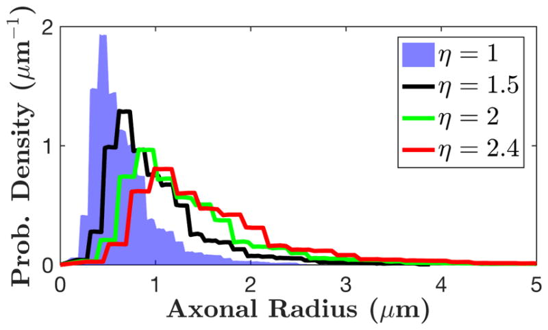
Histogram of axonal radii h_i = h(r_i), based on histological results in corpus callosum of three post-mortem human brains (Caminiti et al., 2009) sampled into 100 bins r_i. The shrinkage factor η extends the bins r_i → ηr_i, modeling a correction for the axonal radii due to a uniform tissue shrinkage during fixation, with η = 1 (blue area) corresponding to no shrinkage, i.e. the measured histogram equal to that in vivo.

Very large apparent axonal diameters would necessarily imply strong brain tissue shrinkage in fixation and paraffin embedding (Horowitz et al., 2015b), such that histologically measured axons have to be assumed notably smaller than in vivo. To compensate for such hypothetical shrinkage, we introduce a shrinkage factorη > 1, which linearly extends the measured radii histogram (Fig. 2 and Appendix A), such that mean axonal radius is η times larger than that calculated with histology. We note from the outset, that η cannot exceed 1.5, as argued in refs. (Aboitiz et al., 1992; Houzel et al., 1994), and η ~ 1.03–1.07 measured in ref. (Tang and Nyengaard, 1997; Tang et al., 1997).

Fig. 3 shows that, in each ROI, the full intra-axonal model (van Gelderen), Eq. (A.3) and Eq. (A.5), can neither fit the scan 1 data nor predict the δ-dependence in scan 2 data if η ≤ 2. (We fixed η to a few values, instead of letting it vary, to achieve fit robustness.) Based on the parameters in Table 3, in most of the ROIs, the values of f_in hit the upper bound and the fits are poor (R² < 0.9) if η ≤ 2. Thus, to fit the data with reasonable parameters and to predict the δ-dependence, the shrinkage due to tissue fixation should exceed two-fold, which contradicts available histological data (Aboitiz et al., 1992; Houzel et al., 1994; Tang and Nyengaard, 1997; Tang et al., 1997).

Figure 3.

D from Fig. 1, fit with full intra-axonal model (van Gelderen), Eq. (A.3) and Eq. (A.5), for the four values of the shrinkage factor η = [1, 1.5, 2, 2.4] (dashed lines, top row). Poor fits for η ≤ 2 are due to f_in hitting the upper bound. Dashed lines in bottom row are predictions (not fits) for δ-dependence in scan 2 data, based on parameters obtained from scan 1 (Table 3 and Eq. A.5). Solid lines in upper and lower rows are the same as those in Fig. 1, i.e. fits for scan 1 and predictions for scan 2 based on Eq. 3 (extra-axonal model), shown here for reference.

Table 3.

Estimated parameters from scan 1, based on intra-axonal model (van Gelderen), Eq. (A.5), fixed at four shrinkage factors η. The range of f_in is [0, 1]. In most of the ROIs, when η ≤ 2, the fitted f_in hits its upper bound, and the fit is poor (R² < 0.9), which is also shown in the upper rows of Fig. 3. To obtain a better fit and ensure f_in < 1, shrinkage factor η needs to exceed 2, which is unrealistic (Aboitiz et al., 1992; Caminiti et al., 2009; Liewald et al., 2014; Houzel et al., 1994; Tang and Nyengaard, 1997; Tang et al., 1997).

ROI	Intra-axonal model (van Gelderen), Eq. (A.5)
	η = 1			η = 1.5			η = 2			η = 2.4
	R2	D∞	fin	R2	D∞	fin	R2	D∞	fin	R2	D∞	fin
ACR	0.145	0.611	1*	0.562	0.608	1*	0.872	0.603	0.901	0.875	0.602	0.510
SCR	0.112	0.534	1*	0.463	0.531	1*	0.903	0.525	1*	0.950	0.522	0.723
PCR	0.076	0.610	1*	0.327	0.607	1*	0.733	0.600	1*	0.933	0.592	1*
PLIC	0.071	0.440	1*	0.312	0.438	1*	0.719	0.433	1*	0.931	0.427	1*
Splenium	0.047	0.368	1*	0.211	0.366	1*	0.527	0.361	1*	0.785	0.354	1*

^*The fitting parameter f_in hits the upper bound.

Interestingly, when η > 2, the functional form of the intraaxonal model (van Gelderen) is very similar to that of our extraaxonal model, i.e. the intra-axonal model begins to describe both the varying Δ and δ data sets equally well. This explains why, in previous studies, which were performed at a few Δ and δ and which did not focus on the functional form of D(Δ, δ), the axonal diameter estimations based on the intra-axonal model alone were much larger than that in histological studies (Alexander et al., 2010; Barazany et al., 2009)—the fitting was “stretching” the axons to match the data. In contrast, the extra-axonal model, Eq. (3), does not stretch the length scales, and provides precise predictions for the δ-dependence, Fig. 1b, and realistic packing correlation length estimates, Table 1.

We also note that for the spinal cord, where axons are about factor of 5 thicker than those in the brain (Peters et al., 1991; Waxman et al., 1995), one must use the full van Gelderen’s model since t_c ~ 10 ms. In this situation, the balance between the intra- and extra-axonal time-dependencies should be revisited, due to the very strong, ~ r⁴ scaling of the intra-axonal signal, so that both effects are now comparable. The dMRI measurement can become sensitive to the inner diameters of the spinal cord WM, and reasonable diameter estimates can be obtained (Benjamini et al., 2016; Komlosh et al., 2013; Duval et al., 2015); however, accounting for the nontrivial time-dependence of the extra-axonal diffusion coefficient still improves such estimates (Xu et al., 2014).

4.2. Relation to measurements with strong diffusion gradients

Applying extremely strong diffusion gradients G ~ 0.1–1 T/m facilitates the estimation of intra-axonal parameters (Barazany et al., 2009; Sepehrband et al., 2016; De Santis et al., 2016; Alexander et al., 2010; Assaf et al., 2008; Huang et al., 2015) because of stronger signal attenuation inside axons, as well as due to exponential suppression of the extra-axonal signal in the radial direction, roughly as $~f_{\text{ex}}{e}^{-b{D}_{\infty }^{\text{ex}}}$.

However, for strong diffusion gradients, the intra-axonal model needs corrections, since the Gaussian phase approximation (GPA) for S_in, under which both Neuman’s and van Gelderen’s solutions were obtained, eventually breaks down. Unfortunately, no solutions beyond GPA currently exist for finite pulse width δ. In Appendix A, Beyond GPA, we estimate that GPA breaks down when

$$g\succsim g^{\ast }=\frac{D_0}{r^3}=\frac{1}{r}·\frac{1}{t_c}.$$ (4)

Recall that the Larmor frequency gradient g ≡ γG is defined via the proton gyromagnetic ratio γ. For reference, g = 0.0107 (μm · ms)⁻¹ for G = 40mT/m (typical human scanner).

Estimating Larmor frequency inhomogeneity across an axon by Ω ~ g^* · r, the above condition becomes Ω · t_c ~ 1, i.e. the typical precession phase during diffusion across an axon is ~ 1 (i.e. not small). Note that the critical gradient g^* is purely determined by tissue properties, independent of sequence timings. For example, if r = 3μm and D₀ = 2μm²/ms, g^* = 0.0741 (μm · ms)⁻¹ (corresponding to G = 277 mT/m); when the actual g becomes of this order of magnitude (and proportionally larger for smaller axons), the higher-order in g corrections to GPA become crucial.

In our experiments, the gradient strength stays below 77 mT/m, and GPA perfectly applies. Recent studies boosted diffusion gradients up to G ≲ 300 mT/m for humans (Huang et al., 2015) and G ≲ 1.3 T/m for ex-vivo mice (Sepehrband et al., 2016). When the signal contribution of large axons is not negligible, beyond-GPA corrections are needed due to the tail of axonal histogram extending to large axons, since for them, the critical g^* decreases as 1/r. The negative beyond-GPA correction to ln S_in, Eq. (A.7), may therefore explain the residual overestimation of axonal diameters in the study (Sepehrband et al., 2016) with ultra-strong gradients—basically, this correction tells that S_in experiences extra attenuation due to the 𝒪(g⁴) contribution, neglected in standard axonal diameter mapping frameworks.

Similarly, higher-order corrections in the powers of diffusion weighting b ∝ g², Eq. (1), should be considered for the extra-axonal signal. The extra-axonal signal S_ex up to 𝒪(b²) can be obtained from the recent narrow-pulse result [Appendix E of ref. (Burcaw et al., 2015)], by substituting t_c → δ as the logarithmic cutoff:

$$ln{S}_{\text{ex}}\simeq -b{D}_{\text{ex}}(\mathrm{\Delta },\delta )+\frac{K_{\text{ex}}}{6}{(b{D}_{\infty }^{\text{ex}})}^2,$$ (5)

where K_ex(Δ, δ) is the apparent extra-axonal kurtosis,

$$\frac{K_{\text{ex}}(\mathrm{\Delta },\delta )}{6}\simeq \frac{A}{D_{\infty }^{\text{ex}}}·\frac{ln(\mathrm{\Delta }/\delta )}{\mathrm{\Delta }},\mathrm{\Delta }\gg \delta \gg t_c.$$

Here, the genuine kurtosis K_ex(t) has the ln(t/t_c)/t tail (Burcaw et al., 2015), and we used the low-pass filter analogy in the wide pulse limit δ ≫ t_c, to re-define the long-time tail cut-off, t_c → δ.

Eq. (5) tells that the 𝒪(b²) kurtosis term becomes of the order of the nontrivial, time-dependent 𝒪(b) term, when $b{D}_{\infty }^{\text{ex}}\succsim 1$; this condition practically coincides with the breakdown of the 𝒪(b), DTI representation ln $S\approx -b·f_{\text{ex}}{D}_{\infty }^{\text{ex}}$, for the total signal $S\simeq f_{\text{in}}+f_{\text{ex}}{e}^{-b{D}_{\infty }^{\text{ex}}}$. In other words, at the same b when the curvature of the observed ln S versus b becomes notable, the extra-axonal K_ex term in Eq. (5) must be included in the analysis if one wants to estimate A and f_in, f_ex (and, possibly the inner radii) separately, by going to high b; one cannot use the approximation S|_Kex≡0 ≃ f_inS_in + f_ex e^{−bD_ex (Δ,δ)} beyond its 𝒪(b) term. De Santis et al. (De Santis et al., 2016) used the S|_Kex≡0 approximation to modify AxCaliber estimation of inner diameters from human brain data in the corpus callosum acquired with stimulated echo dMRI with b ≤ 4ms/μm². Including the D_ex(Δ, δ) term in Eq. (5) resulted in about 5-fold smaller inner diameter estimates in comparison to just using $D_{\infty }^{\text{ex}}$, effectively demonstrating the importance of non-Gaussian (time-dependent) extra-axonal space contribution to the total signal, consistent with ref. (Fieremans et al., 2016). However, δ was fixed to a single value while Δ varied, even though S_in mostly depends on δ, and Δ-dependence drops out in the Neuman’s limit, cf. Appendix A. Omission of the equally important K_ex contribution (as well as, possibly, higher-order cumulant terms) has introduced an unknown bias into parameter estimation.

Here, we limited our analysis to b ≤ 0.5ms/μm² to stay in the linear, DTI regime of Eq. (1). We therefore cannot estimate A and compartment fractions separately; such estimation would require a systematic measurement of both Δ and δ dependencies at higher b, and including higher-order cumulants into the model for S_ex(Δ, δ; b). This is beyond the scope of the present work. We also attempted to fit to scan 1 data a hybrid model D = f_inD_in(Δ, δ) + f_exD_ex(Δ, δ), including finite axonal radius histogram in the van Gelderen’s framework of D_in(Δ, δ); fitting results were unstable, and corresponding parameters were highly dependent on their initial values, signifying a “shallow direction” in the fitting landscape. Such spurious parameter correlation should be expected from similar functional forms of the extra-axonal model and of the intraaxonal (van Gelderen) model for large inner radii, cf. Fig. 3 for large η.

4.3. Limitations

To simplify models and interpretations, we ignored the fiber orientation dispersion, which is generally non-negligible in the brain WM (Zhang et al., 2011; Alexander et al., 2010; Veraart et al., 2016b). The orientation dispersion may project part of the axial diffusivity time-dependence to the radial direction, increasing estimated c and c′, and also the microstructural length scale, 2r̄ and $l_c^{\perp }$ (Fieremans et al., 2016). In the future, it may be possible to consistently factor out this dispersion by generalizing the rotationally-invariant parameter framework (Novikov et al., 2016b; Reisert et al., 2017) onto time-dependent diffusion propagators.

To ensure the SNR sufficient for the model selection, we used a relatively large voxel size, leading to partial volume effects in some ROIs. For example, diffusivities in the genu and midbody of the CC have no significant time dependence since they are very close to the CSF, and vulnerable to the CSF signal contamination and potentially CSF pulsations. Because of the same reason, the time dependence in the splenium is noisier than in other ROIs with significant time dependences, shown in Fig. 1 and Table 1 (higher P-value for splenium).

We also ignored the effect of T₁ differences between intraand extra-axonal water, and water in-between myelin sheath. To minimize this effect, we applied the same TR for all measurements, and used a relatively long TR.

Due to the observable T₂ differences between intra- and extra-axonal water (Veraart et al., 2017), volume fractions (f_in, f_ex) are T₂-weighted. By applying the same TE throughout the measurements, this effect was fixed and did not change the functional form of diffusion time-dependence.

We ignored the water exchange between intra- and extraaxonal water, and water in-between myelin sheath. To reduce the influence of water exchange between different compartments, we used a spin-echo sequence (T₂-weighted), rather than a stimulated- echo one (T₁-, T₂-weighted), since the time scale of T₁ relaxation and water exchange is comparable in the brain (~ 1 sec), and could confound measurements (Deoni et al., 2008; Lampinen et al., 2017).

4.4. Correlation of dMRI with axonal conduction velocity

Generally, thicker axons have higher axonal conduction velocity (ACV), by optimizing the ratio of internode length to fiber diameter (Rushton, 1951). A relevant question is whether it is inner or outer axonal diameter, or some combination of both, that determine ACV most definitively. Hursh (1939) observed that, in the peripheral nerve of cats and kittens, the ACV was linearly correlated with the outer axonal diameter. On the other hand, Gasser and Grundfest (1939) performed a similar experiment and argued that, in the peripheral nerve of cats and rabbits, ACV was linearly correlated with the inner axonal diameter. Rushton (1951) and Waxman and Bennett (1972) reanalyzed Hursh’s data, and all concluded that ACV is proportional to the outer diameter. However, Sanders and Whitteridge’s (1946) results in rabbit’s peroneal nerve showed that the myelin sheath thickness, i.e. the difference between outer and inner radii, had the highest correlation with ACV, rather than inner and outer diameters separately. Arbuthnott et al. (1980) studied the peripheral nerve of cat and suggested that conduction velocity is proportional to inner diameter; however, they did not measure the conduction velocity in this study, and the conclusion was made based on their theoretical discussion. To estimate the ACV in the human brain, Aboitiz et al. (1992) assumed that inner diameter has a linear relationship with ACV; the proportionality constant is 8.7 mm/ms per μm of inner diameter, which is calculated in the peripheral nervous system (Ruch and Patton, 1982). Also, ACV is highly affected by myelination (Castelfranco and Hartline, 2016), such as myelin sheath thickness and internode length, prompting more advanced models for estimating ACV.

The advent of in vivo dMRI has offered an exciting proposition to map axonal diameters, and to study in vivo the decadesold relation between axonal sizes and ACV. In 2014, based on the AxCaliber interpretation of dMRI, Horowitz et al. (2015a) estimated apparent inner axonal diameters in the in vivo human brain, and displayed their correlation with ACV measured with electroencephalography; the estimated proportionality constant was close to the value used by Aboitiz et al. (1992) (Ruch and Patton, 1982). The finding was subsequently criticized by Innocenti, Caminiti, and Aboitiz (2015) since the estimated inner diameter was much larger than histological observations, and the measured interhemispheric transfer time was much shorter than the value in previous literature. This debate presents an interesting scientific question: Can one rationalize fairly strong apparent correlations between dMRI and ACV observed by Horowitz et al. (2015a) with the inconsistencies of inner diameter estimation methodology?

The relevance of the nontrivial dMRI signal from the extra-axonal space leads us to posit that the correlation uncovered by Horowitz et al. (2015a) is, to the leading order 𝒪(b), between the strength of time dependence (c or c′ in Eq. (2) or Eq. (3)), and ACV. Interpreting the strength of time dependence as inner diameter or extra-axonal packing correlation length depends on the model selection. Our present model selection results suggest re-interpreting dMRI axonal diameter mapping in terms of the dominant extra-axonal contribution, defined in terms of the “disorder strength” A, and the related axonal packing correlation length $l_c^{\perp }~\sqrt{A}~\sqrt{c^{\prime }}$ estimating outer diameters. Selecting the extra-axonal model based on our current data is then consistent with the above mentioned correlations (Hursh, 1939;Waxman and Bennett, 1972; Rushton, 1951; Sanders and Whitteridge, 1946) between, predominantly, the outer axonal diameters and ACV.

5. Conclusions

We considered the functional form of D(Δ, δ) for two plausible biophysical models with mutually exclusive physical assumptions. We experimentally showed in the in vivo human brain, that the extra-axonal model provides a far better agreement with the measurement, both in terms of the quality of its parameter-free prediction of the measurement with varying δ, and in terms of the qualitative ln(1/δ), rather than 1/δ, functional form. Varying δ has revealed a nontrivial low-pass filter effect of the gradient duration on the genuine molecular diffusion coefficient D(t).

Extra-axonal model provides reasonable values of the packing correlation length, which is compatible to the scale of outer axonal diameter. In contrast, intra-axonal model alone overestimates the inner axonal diameters by at least twofold as compared with histology, which cannot be explained by any reasonable degree of the tissue shrinkage in fixation.

The sensitivity of time-dependent diffusion to packing geometry of the extra-axonal space may serve as a marker for demyelination or axonal loss in neurodegenerative diseases. Our results are also consistent with the correlations between outer axonal diameter and axonal conduction velocity.

Supplementary Material

1

Figure S.1: Five subjects’ radial diffusivities D in scan 1 within seven WM ROIs with respect to diffusion time Δ.

2

Figure S.2: Five subjects’ radial diffusivities D in scan 2 within seven WM ROIs with respect to diffusion gradient pulse width δ.

3

Figure S.3: Five subjects’ probability density functions (PDFs) of radial diffusivities D in scan 1 within seven WM ROIs with respect to diffusion time Δ.

4

Figure S.4: Five subjects’ probability density functions (PDFs) of radial diffusivities D in scan 2 within seven WM ROIs with respect to diffusion gradient pulse width δ.

5

Figure S.5: Radial diffusivity D(Δ, δ) for WM ROIs averaged over five subjects (a data set different from the main text). (a) With fixed δ = 15 ms, D from scan 1 decreases with Δ. Dashed and solid lines are fits based on Eq. (2) (intra-axonal) and Eq. (3) (extra-axonal), correspondingly. (b) With fixed Δ = 55 ms, D from scan 2 increases as a function of 1/δ. Dashed and solid lines are predictions (not fits) based on parameters obtained from scan 1 (Table S.1), using the corresponding models, Eq. (2) and Eq. (3).

6

Figure S.6: Radial diffusivity D(Δ, δ) for WM ROIs averaged over five subjects (a data set different from the main text). (a) With fixed δ = 15 ms, D from scan 1 decreases with Δ. Dashed and solid lines are predictions (not fits) based on parameters obtained from scan 2 (Table S.2), using the corresponding models, Eq. (2) (intra-axonal) and Eq. (3) (extra-axonal). (b) With fixed Δ = 55 ms, D from scan 2 increases as a function of 1/δ. Dashed and solid lines are fits based on Eq. (2) and Eq. (3), correspondingly.

7

Table S.1: Estimated parameters from scan 1 (a data set different from the main text), based on intra-axonal model, Eq. (2), and extra-axonal model, Eq. (3). Intra-axonal model: Values of 2r̄ (f_in/D₀)^1/4 and η̄ (f_in/D₀)^1/4 are lower bounds of, respectively, the (volume-weighted) inner axonal diameter 2r̄ (cf. text below Eq. (2)), and of the axonal shrinkage η̄ (Fig. 2 and Eq. (A.2)) since, practically, f_in/D₀ < 1ms/μm². The 2r̄|_{D0, fin} and η̄|_{D0, fin} are calculated by using typical values of f_in = 0.5 and D₀ = 2μm²/ms. Extra-axonal model: We used empirical estimate (Burcaw et al., 2015) $A\approx 0.2{(l_c^{\perp })}^2$, to obtain the combination $l_c^{\perp }\sqrt{f_{\text{ex}}}$ from c′. This sets a lower bound (Fieremans et al., 2016) on the fiber packing correlation length $l_c^{\perp }$ because f_ex < 1; $l_c^{\perp }$ provides an estimate for the outer axonal diameter. Standard deviations are shown in the parenthesis. All parameters are in the corresponding units of μm and ms.

Table S.2: Estimated parameters from scan 2 (a data set different from the main text), based on intra-axonal model, Eq. (2), and extra-axonal model, Eq. (3). Intra-axonal model: Values of 2r̄ (f_in/D₀)^1/4 and η̄ (f_in/D₀)^1/4 are lower bounds of, respectively, the (volume-weighted) inner axonal diameter 2r̄ (cf. text below Eq. (2)), and of the axonal shrinkage η̄ (Fig. 2 and Eq. (A.2)) since, practically, f_in/D₀ < 1ms/μm². The 2r̄|_{D0, fin} and η̄|_{D0, fin} are calculated by using typical values of f_in = 0.5 and D₀ = 2μm²/ms. Extra-axonal model: We used empirical estimate (Burcaw et al., 2015) $A\approx 0.2{(l_c^{\perp })}^2$, to obtain the combination $l_c^{\perp }\sqrt{f_{\text{ex}}}$ from c′. This sets a lower bound (Fieremans et al., 2016) on the fiber packing correlation length $l_c^{\perp }$ because f_ex < 1; $l_c^{\perp }$ provides an estimate for the outer axonal diameter. Standard deviations are shown in the parenthesis. All parameters are in the corresponding units of μm and ms.

Appendix A. Intra-axonal model

Here we obtain qualitative estimates for signal attenuation within an impermeable cylinder in the GPA, outline exact relations for D_in(Δ, δ) in different limits, and estimate when GPA breaks down.

Mapping onto transverse relaxation

Fundamentally, dMRI is a measurement of transverse NMR relaxation in the applied diffusion gradient. Each spin, following its Brownian path x(τ ), contributes the precession phase e^−iϕ(t), $\varphi (t)={\int }_0^t\mathrm{\Omega }(\mathbf{x}(\tau ),\tau )\mathrm{d}\tau$, where Ω(x, τ) is the local Larmor frequency offset (relative to γB₀), that also depends on time τ explicitly due to the time-varying applied gradient. The dMRI signal S = 〈e^−iϕ〉 ≡ p(λ)|_λ=1, given by the average over all spins in a voxel, is, effectively, the Fourier transform p(λ) = 〈e^−iλϕ〉 of the probability density function ℘(ϕ) of all possible precession phases ϕ(t), where 〈 … 〉 is the average with respect to ℘(ϕ).

Wide-pulse limit in the GPA

Generally, the form of ℘(ϕ) is quite complicated, and is mediated by the diffusion (Kiselev and Posse, 1998; Jensen and Chandra, 2000; Sukstanskii and Yablonskiy, 2003, 2004; Novikov and Kiselev, 2008). Fortunately, in the wide-pulse limit δ ≫ t_c, the problem of finding its Fourier transform p(λ) simplifies, as the problem maps onto that of transverse relaxation in the diffusion-narrowing regime (equivalent to the GPA). In this limit, the time t_c to diffuse across an axon of radius r provides the correlation time, beyond which the contribution to the precession phase ϕ for each spin gets randomized. It is then natural to split each Brownian path x(τ ) into N = t/t_c ≫ 1 steps of duration t_c, such that the total phase can be estimated as $\varphi ~{\sum }_{n=1}^N{\varphi }_n$, where each ϕ_n ~ Ω · t_c can be treated as an independent random variable with zero mean and variance $\langle {\varphi }_n^2\rangle ~{(\mathrm{\Omega }·t_c)}^2$; here Ω ~ g · r is a typical value of the Larmor frequency inhomogeneity across an axon imposed by the applied gradient g. When the number N of independent “steps” becomes large, the Central limit theorem (CLT) tells that the characteristic function p(λ) ≃ e^{−iλ〈ϕ〉−λ2〈ϕ2〉_c/2} approaches that of the Gaussian distribution, with the higher-order cumulants being less relevant. Moreover, according to the CLT, the mean values and variances from the independent steps add up, i.e. 〈ϕ〉 ≡ 0, and ${\langle {\varphi }^2\rangle }_c\equiv \langle {\varphi }^2\rangle -{\langle \varphi \rangle }^2~N\langle {\varphi }_n^2\rangle ~{\mathrm{\Omega }}^2{t}_c·t$, such that $S_{\text{in}}~e^{-R_2^{\ast }·t}$, with effective $R_2^{\ast }~{\mathrm{\Omega }}^2{t}_c$, cf. refs. (Kiselev and Posse, 1998; Jensen and Chandra, 2000; Sukstanskii and Yablonskiy, 2003, 2004; Novikov and Kiselev, 2008). In our case, it is the total pulse duration t = 2δ that matters; note that the inter-pulse duration Δ ≥ δ does not enter these considerations, as long as δ ≫ t_c, since Ω(x, τ) ≡ 0 and no transverse relaxation occurs during the time when the gradient is off. Hence, the 𝒪(g²) attenuation inside an axon scales as $-ln{S}_{\text{in}}\simeq \frac{1}{2}{\langle {\varphi }^2\rangle }_c~(g^2{r}^4/D_0)·\delta$, which indeed agrees with the 1974 exact calculation of Neuman (1974)

$$-ln{S}_{\text{in}}=\frac{7}{48}·\frac{g^2{r}^4}{D_0}·\delta +\mathcal{O}(g^4),$$ (A.1)

where the coefficient 7/48 is specific to the assumed perfectly circular cylinder cross-section.

Factoring out b in Eq. (A.1), cf. Eq. (1), leads to the intraaxonal contribution in Eq. (2). The corresponding D_in is about 4 × 10⁻⁵ − 2 × 10⁻⁴ μm²/ms for r ~ 1 μm, D₀ = 2μm²/ms, Δ = 26–100 ms, and δ = 20ms, being much smaller than the measured diffusivity change in our experiment; to account for the observed diffusivity variation over diffusion times, apparent radii r̄ need to be much larger, cf. Table 1.

The estimated shrinkage factor for apparent radii r̄ in the Neuman’s regime is

$$\overline{\eta }\equiv \frac{\overline{r}}{1.48\mu \mathrm{m}},$$ (A.2)

where the denominator is the apparent radius ${(\langle r^6\rangle /\langle r^2\rangle )}^{\frac{1}{4}}$ calculated via the histology histogram (Caminiti et al., 2009), the blue area in Fig. 2.

General solution in the GPA

When Neuman’s assumption δ ≫ t_c is not satisfied, one needs to use the general 𝒪(g²) solution for signal attenuation inside a cylinder of radius r by van Gelderen et al. (1994):

$$-ln{S}_{in}^{\text{vG}}(\mathrm{\Delta },\delta ;r)=\frac{2g^2{r}^4}{D_0}\sum _{m=1}^{\infty }\frac{t_c}{{\alpha }_m^6({\alpha }_m^2-1)}·[2{\alpha }_m^2\frac{\delta }{t_c}-2+2e^{-{\alpha }_m^2\delta /t_c}+2e^{-{\alpha }_m^2\mathrm{\Delta }/t_c}-e^{-{\alpha }_m^2(\mathrm{\Delta }-\delta )/t_c}-e^{-{\alpha }_m^2(\mathrm{\Delta }+\delta )/t_c}]$$ (A.3)

where α_m is the m^th root of dJ₁(α)/dα = 0, and J₁(α) is the Bessel function of the first kind; note that t_c = t_c(r) = r²/D₀. In the δ ≫ t_c limit, the Δ-dependence drops out, and Eq. (A.3) approaches Eq. (A.1). In the opposite, narrow-pulse limit δ ≪ t_c, ln S_in(t, δ; r)|_δ=0 = –bD(t), with D(t) = r²/(4t).

In our analysis, we incorporate the axonal radius histogram from the corpus callosum of three post-mortem human brains, by Caminiti et al. (2009), Fig. 2, and allow for the uniform axonal stretching, r_i → ηr_i, such that the overall intra-axonal signal for a given shrinkage factor η is the volume-averaged Eq. (A.3)

$$S_{\text{in}}(\mathrm{\Delta },\delta ;\eta )=\sum _i{f}_i{S}_{\text{in}}^{\text{vG}}(\mathrm{\Delta },\delta ;\eta r_i)$$ (A.4)

with the normalized weights $f_i=h_i{r}_i^2/{\sum }_j{h}_j{r}_j^2$ given in terms of the histogram bin values h_i. The effective $D_{\text{in}}^{\text{vGel}}(\mathrm{\Delta },\delta ;\eta )$ is obtained by factoring out the b-value from ln S_in, cf. Eq. (1). The average radius is 〈r〉 ~ 0.67 μm ×η according to the weights h_i. The value of g² is estimated by the b-value defined in Eq. (1). The intra-axonal model based on van Gelderen et al. ’s solution then yields

$$D^{\text{vGel}}(\mathrm{\Delta },\delta ;\eta )=D_{\infty }+f_{\text{in}}{D}_{\text{in}}^{\text{vGel}}(\mathrm{\Delta },\delta ;\eta ).$$ (A.5)

This model includes four parameters: D_∞, f_in, η, and D₀. To stabilize our fitting, we fixed D₀ by the value of the axial diffusivity D_|| from the diffusion tensor, and fixed η at a few values [1, 1.5, 2, 2.4]. After that, we only have two fitted parameters, D_∞ and f_in, estimated from scan 1 data, in Table 3. Using these parameters, we predicted the δ-dependence in scan 2 results based on Eq. (A.5) without tunable parameters, shown in Fig. 3.

Beyond GPA

Unfortunately, there are no exact results for the 𝒪(g⁴) terms and beyond in Eq. (A.1). Let us estimate this next-order term using similar qualitative considerations as above, and establish where the GPA breaks down. For that, we need to estimate the 4th-order cumulant 〈ϕ⁴〉_c ≡ 〈ϕ⁴〉 − 3〈ϕ²〉² of the precession phase in the cumulant expansion (Kiselev, 2010) of p(λ) taken at λ ≡ 1:

$$lnS=-\frac{1}{2!}{\langle {\varphi }^2\rangle }_c+\frac{1}{4!}{\langle {\varphi }^4\rangle }_c-\dots .$$ (A.6)

By definition of the kurtosis K of the phase distribution ℘(ϕ), ${\langle {\varphi }^4\rangle }_c=K·{\langle {\varphi }^2\rangle }_c^2$. In the large-N limit, kurtosis scales as K ~ −1/N ~ –t_c/δ and is negative as a result of the confined intra-axonal geometry (see the derivation in Supplementary Information, Section I). As a result, we obtain

$${\langle {\varphi }^4\rangle }_c~-\frac{g^4{r}^{10}}{D_0^3}·\delta .$$ (A.7)

GPA breaks down when 〈ϕ⁴〉_c ~ 〈ϕ²〉_c in Eq. (A.6), equivalent to 〈ϕ²〉_c ~ δ/t_c, from which the breakdown condition, Eq. (4) in the main text, follows. For such strong gradients, all terms in cumulant expansion are of the same order, which requires development of non-perturbative approaches.

References

- Aboitiz F, Scheibel AB, Fisher RS, Zaidel E. Fiber composition of the human corpus callosum. Brain Res. 1992;598(1–2):143–153. doi: 10.1016/0006-8993(92)90178-c. URL http://www.ncbi.nlm.nih.gov/pubmed/1486477. [DOI] [PubMed] [Google Scholar]
- Ackerman JJH, Neil JJ. The use of MR-detectable reporter molecules and ions to evaluate diffusion in normal and ischemic brain. NMR Biomed. 2010 Aug;23(7):725–33. doi: 10.1002/nbm.1530. [DOI] [PMC free article] [PubMed] [Google Scholar]
- Alexander DC, Hubbard PL, Hall MG, Moore EA, Ptito M, Parker GJ, Dyrby TB. Orientationally invariant indices of axon diameter and density from diffusion MRI. Neuroimage. 2010;52(4):1374–1389. doi: 10.1016/j.neuroimage.2010.05.043. URL http://www.ncbi.nlm.nih.gov/pubmed/20580932. [DOI] [PubMed] [Google Scholar]
- Andersson JL, Jenkinson M, Smith S. Report, FMRIB Analysis Group of the University of Oxford. 2007. Non-linear registration, aka Spatial normalisation FMRIB technical report TR07JA2. [Google Scholar]
- Andersson JL, Sotiropoulos SN. An integrated approach to correction for off-resonance effects and subject movement in diffusion MR imaging. Neuroimage. 2016;125:1063–1078. doi: 10.1016/j.neuroimage.2015.10.019. URL http://www.ncbi.nlm.nih.gov/pubmed/26481672. [DOI] [PMC free article] [PubMed] [Google Scholar]
- Arbuthnott ER, Boyd IA, Kalu KU. Ultrastructural dimensions of myelinated peripheral nerve fibres in the cat and their relation to conduction velocity. J Physiol. 1980;308:125–157. doi: 10.1113/jphysiol.1980.sp013465. URL http://www.ncbi.nlm.nih.gov/pubmed/7230012. [DOI] [PMC free article] [PubMed] [Google Scholar]
- Åslund I, Topgaard D. Determination of the self-diffusion coefficient of intracellular water using PGSE NMR with variable gradient pulse length. Journal of Magnetic Resonance. 2009;201(2):250– 254. doi: 10.1016/j.jmr.2009.09.006. URL http://www.sciencedirect.com/science/article/pii/S1090780709002626. [DOI] [PubMed] [Google Scholar]
- Assaf Y, Basser PJ. Composite hindered and restricted model of diffusion (CHARMED) MR imaging of the human brain. NeuroImage. 2005;27(1):48– 58. doi: 10.1016/j.neuroimage.2005.03.042. URL http://www.sciencedirect.com/science/article/pii/S1053811905002259. [DOI] [PubMed] [Google Scholar]
- Assaf Y, Blumenfeld-Katzir T, Yovel Y, Basser PJ. AxCaliber: a method for measuring axon diameter distribution from diffusion MRI. Magn Reson Med. 2008;59(6):1347–1354. doi: 10.1002/mrm.21577. URL http://www.ncbi.nlm.nih.gov/pubmed/18506799. [DOI] [PMC free article] [PubMed] [Google Scholar]
- Bando Y, Nomura T, Bochimoto H, Murakami K, Tanaka T, Watanabe T, Yoshida S. Abnormal morphology of myelin and axon pathology in murine models of multiple sclerosis. Neurochemistry International. 2015;81:16– 27. doi: 10.1016/j.neuint.2015.01.002. URL http://www.sciencedirect.com/science/article/pii/S0197018615000066. [DOI] [PubMed] [Google Scholar]
- Bar-Shir A, Cohen Y. High b-value q-space diffusion MRS of nerves: structural information and comparison with histological evidence. NMR in Biomedicine. 2008;21(2):165–174. doi: 10.1002/nbm.1175. URL . [DOI] [PubMed] [Google Scholar]
- Barazany D, Basser P, Assaf Y. In vivo measurement of axon diameter distribution in the corpus callosum of rat brain. Brain. 2009;132:1210–1220. doi: 10.1093/brain/awp042. [DOI] [PMC free article] [PubMed] [Google Scholar]
- Basser PJ, Mattiello J, LeBihan D. MR diffusion tensor spectroscopy and imaging. Biophysical Journal. 1994;66(1):259–267. doi: 10.1016/S0006-3495(94)80775-1. URL . [DOI] [PMC free article] [PubMed] [Google Scholar]
- Benjamini D, Komlosh ME, Holtzclaw LA, Nevo U, Basser PJ. White matter microstructure from nonparametric axon diameter distribution mapping. NeuroImage. 2016;135:333– 344. doi: 10.1016/j.neuroimage.2016.04.052. URL http://www.sciencedirect.com/science/article/pii/S1053811916300921. [DOI] [PMC free article] [PubMed] [Google Scholar]
- Burcaw LM, Fieremans E, Novikov DS. Mesoscopic structure of neuronal tracts from time-dependent diffusion. Neuroimage. 2015;114:18–37. doi: 10.1016/j.neuroimage.2015.03.061. URL http://www.ncbi.nlm.nih.gov/pubmed/25837598. [DOI] [PMC free article] [PubMed] [Google Scholar]
- Callaghan PT. Principles of Nuclear Magnetic Resonance Microscopy. Clarendon; Oxford: 1991. [Google Scholar]
- Caminiti R, Ghaziri H, Galuske R, Hof PR, Innocenti GM. Evolution amplified processing with temporally dispersed slow neuronal connectivity in primates. Proc Natl Acad Sci USA. 2009;106(46):19551–19556. doi: 10.1073/pnas.0907655106. URL http://www.ncbi.nlm.nih.gov/pubmed/19875694. [DOI] [PMC free article] [PubMed] [Google Scholar]
- Castelfranco AM, Hartline DK. Evolution of rapid nerve conduction. Brain Research. 2016;1641(Part A):11–33. doi: 10.1016/j.brainres.2016.02.015. evolution of Myelin. URL http://www.sciencedirect.com/science/article/pii/S0006899316300580. [DOI] [PubMed] [Google Scholar]
- Chomiak T, Hu B. What is the optimal value of the g-ratio for myelinated fibers in the rat CNS? A theoretical approach. PLoS One. 2009;4(11):e7754. doi: 10.1371/journal.pone.0007754. URL http://www.ncbi.nlm.nih.gov/pubmed/19915661. [DOI] [PMC free article] [PubMed] [Google Scholar]
- De Santis S, Jones DK, Roebroeck A. Including diffusion time dependence in the extra-axonal space improves in vivo estimates of axonal diameter and density in human white matter. Neuroimage. 2016;130:91–103. doi: 10.1016/j.neuroimage.2016.01.047. URL http://www.ncbi.nlm.nih.gov/pubmed/26826514. [DOI] [PMC free article] [PubMed] [Google Scholar]
- Deoni SC, Rutt BK, Arun T, Pierpaoli C, Jones DK. Gleaning multicomponent T1 and T2 information from steady-state imaging data. Magnetic Resonance in Medicine. 2008;60(6):1372–1387. doi: 10.1002/mrm.21704. URL . [DOI] [PubMed] [Google Scholar]
- Duval T, McNab JA, Setsompop K, Witzel T, Schneider T, Huang SY, Keil B, Klawiter EC, Wald LL, Cohen-Adad J. In vivo mapping of human spinal cord microstructure at 300mT/m. NeuroImage. 2015;118(Supplement C):494– 507. doi: 10.1016/j.neuroimage.2015.06.038. URL http://www.sciencedirect.com/science/article/pii/S1053811915005418. [DOI] [PMC free article] [PubMed] [Google Scholar]
- Ernst MH, Machta J, Dorfman JR, van Beijeren H. Long-time tails in stationary random media. 1. Theory. Journal of Statistical Physics. 1984;34(3–4):477–495. [Google Scholar]
- Fieremans E, Burcaw LM, Lee HH, Lemberskiy G, Veraart J, Novikov DS. In vivo observation and biophysical interpretation of time-dependent diffusion in human white matter. Neuroimage. 2016;129:414–427. doi: 10.1016/j.neuroimage.2016.01.018. URL http://www.ncbi.nlm.nih.gov/pubmed/26804782. [DOI] [PMC free article] [PubMed] [Google Scholar]
- Gasser HS, Grundfest H. Axon diameters in relation to the spike dimensions and the conduction velocity in mammalian A fibers. American Journal of Physiology–Legacy Content. 1939;127(2):393–414. [Google Scholar]
- Horowitz A, Barazany D, Tavor I, Bernstein M, Yovel G, Assaf Y. In vivo correlation between axon diameter and conduction velocity in the human brain. Brain Struct Funct. 2015a;220(3):1777–1788. doi: 10.1007/s00429-014-0871-0. URL http://www.ncbi.nlm.nih.gov/pubmed/25139624. [DOI] [PubMed] [Google Scholar]
- Horowitz A, Barazany D, Tavor I, Yovel G, Assaf Y. Response to the comments on the paper by Horowitz et al.(2014) Brain Structure and Function. 2015b;220(3):1791. doi: 10.1007/s00429-015-1031-x. [DOI] [PubMed] [Google Scholar]
- Horsfield MA, Barker GJ, McDonald WI. Self-diffusion in CNS tissue by volume-selective proton NMR. Magnetic Resonance in Medicine. 1994;31(6):637–644. doi: 10.1002/mrm.1910310609. URL . [DOI] [PubMed] [Google Scholar]
- Houzel JC, Milleret C, Innocenti G. Morphology of callosal axons interconnecting areas 17 and 18 of the cat. Eur J Neurosci. 1994;6(6):898–917. doi: 10.1111/j.1460-9568.1994.tb00585.x. URL http://www.ncbi.nlm.nih.gov/pubmed/7952278. [DOI] [PubMed] [Google Scholar]
- Huang SY, Nummenmaa A, Witzel T, Duval T, Cohen-Adad J, Wald LL, McNab JA. The impact of gradient strength on in vivo diffusion mri estimates of axon diameter. Neuroimage. 2015;106:464–472. doi: 10.1016/j.neuroimage.2014.12.008. URL http://www.ncbi.nlm.nih.gov/pubmed/25498429. [DOI] [PMC free article] [PubMed] [Google Scholar]
- Hursh JB. Conduction velocity and diameter of nerve fibers. American Journal of Physiology. 1939;127(1):131–139. URL <GotoISI>://WOS:000202435900013. [Google Scholar]
- Innocenti GM, Caminiti R, Aboitiz F. Comments on the paper by Horowitz et al. (2014) Brain Struct Funct. 2015;220(3):1789–1790. doi: 10.1007/s00429-014-0974-7. URL http://www.ncbi.nlm.nih.gov/pubmed/25579065. [DOI] [PubMed] [Google Scholar]
- Jenkinson M, Bannister P, Brady M, Smith S. Improved optimization for the robust and accurate linear registration and motion correction of brain images. Neuroimage. 2002;17(2):825–841. doi: 10.1016/s1053-8119(02)91132-8. URL http://www.ncbi.nlm.nih.gov/pubmed/12377157. [DOI] [PubMed] [Google Scholar]
- Jenkinson M, Smith S. A global optimisation method for robust affine registration of brain images. Med Image Anal. 2001;5(2):143–156. doi: 10.1016/s1361-8415(01)00036-6. URL http://www.ncbi.nlm.nih.gov/pubmed/11516708. [DOI] [PubMed] [Google Scholar]
- Jensen JH, Chandra R. NMR relaxation in tissues with weak magnetic inhomogeneities. Magn Reson Med. 2000 Jul;44(1):144–56. [PubMed] [Google Scholar]
- Jensen JH, Helpern JA, Ramani A, Lu H, Kaczynski K. Diffusional kurtosis imaging: The quantification of non-gaussian water diffusion by means of magnetic resonance imaging. Magnetic Resonance in Medicine. 2005;53(6):1432–1440. doi: 10.1002/mrm.20508. URL . [DOI] [PubMed] [Google Scholar]
- Jones DK. Diffusion MRI: Theory, Methods, and Applications. Oxford University Press; New York: 2011. [Google Scholar]
- Kellner E, Dhital B, Kiselev VG, Reisert M. Gibbs-ringing artifact removal based on local subvoxel-shifts. Magn Reson Med. 2016;76(5):1574–1581. doi: 10.1002/mrm.26054. URL http://www.ncbi.nlm.nih.gov/pubmed/26745823. [DOI] [PubMed] [Google Scholar]
- Kiselev VG. The cumulant expansion: an overarching mathematicl framework for understanding diffusion NMR. In: Jones D, editor. Diffusion MRI: theory, methods, and applications. Ch. 10. Oxford University Press; 2010. pp. 152–168. [Google Scholar]
- Kiselev VG. Fundamentals of diffusion MRI physics. NMR in Biomedicine. 2017 doi: 10.1002/nbm.3602. doi: 10.1002/nbm.3602. URL . [DOI] [PubMed]
- Kiselev VG, Posse S. Analytical theory of susceptibility induced NMR signal dephasing in a cerebrovascular network. Physical Review Letters. 1998;81(25):5696. [Google Scholar]
- Komlosh M, Ã-zarslan E, Lizak M, Horkayne-Szakaly I, Freidlin R, Horkay F, Basser P. Mapping average axon diameters in porcine spinal cord white matter and rat corpus callosum using d-PFG MRI. NeuroImage. 2013;78:210– 216. doi: 10.1016/j.neuroimage.2013.03.074. URL http://www.sciencedirect.com/science/article/pii/S1053811913003273. [DOI] [PMC free article] [PubMed] [Google Scholar]
- Kunz N, Sizonenko SV, Hüppi PS, Gruetter R, van de Looij Y. Investigation of field and diffusion time dependence of the diffusion-weighted signal at ultrahigh magnetic fields. NMR in Biomedicine. 2013;26(10):1251–1257. doi: 10.1002/nbm.2945. URL . [DOI] [PubMed] [Google Scholar]
- Lampinen B, Szczepankiewicz F, van Westen D, Englund E, Sundgren CP, Lätt J, Ståhlberg F, Nilsson M. Optimal experimental design for filter exchange imaging: Apparent exchange rate measurements in the healthy brain and in intracranial tumors. Magnetic Resonance in Medicine. 2017;77(3):1104–1114. doi: 10.1002/mrm.26195. URL . [DOI] [PMC free article] [PubMed] [Google Scholar]
- Liewald D, Miller R, Logothetis N, Wagner HJ, Schuz A. Distribution of axon diameters in cortical white matter: an electron-microscopic study on three human brains and a macaque. Biol Cybern. 2014;108(5):541–557. doi: 10.1007/s00422-014-0626-2. URL http://www.ncbi.nlm.nih.gov/pubmed/25142940. [DOI] [PMC free article] [PubMed] [Google Scholar]
- Mackay A, Whittall K, Adler J, Li D, Paty D, Graeb D. In vivo visualization of myelin water in brain by magnetic resonance. Magnetic Resonance in Medicine. 1994;31(6):673–677. doi: 10.1002/mrm.1910310614. URL . [DOI] [PubMed] [Google Scholar]
- Mitra PP, Sen PN, Schwartz LM, Le Doussal P. Diffusion propagator as a probe of the structure of porous media. Physical Review Letters. 1992 Jun;68(24):3555–3558. doi: 10.1103/PhysRevLett.68.3555. [DOI] [PubMed] [Google Scholar]
- Mori S, Wakana S, Van Zijl PC, Nagae-Poetscher L. MRI atlas of human white matter. Elsevier; Amsterdam, The Netherlands: 2005. [Google Scholar]
- Neuman CH. Spin-echo of spins diffusing in a bounded medium. Journal of Chemical Physics. 1974;60(11):4508–4511. URL <GotoISI>://WOS:A1974T286300056. [Google Scholar]
- Nilsson M, LÃtt J, Nordh E, Wirestam R, StÃhlberg F, Brockstedt S. On the effects of a varied diffusion time in vivo: is the diffusion in white matter restricted? Magnetic Resonance Imaging. 2009;27(2):176– 187. doi: 10.1016/j.mri.2008.06.003. URL http://www.sciencedirect.com/science/article/pii/S0730725X08002014. [DOI] [PubMed] [Google Scholar]
- Novikov DS, Fieremans E. Relating extracellular diffusivity to cell size distribution and packing density as applied to white matter. Proceedings of the 20th Annual Meeting of ISMRM; Melbourne, Victoria, Australia. 2012. p. 1829. [Google Scholar]
- Novikov DS, Jensen JH, Helpern JA, Fieremans E. Revealing mesoscopic structural universality with diffusion. Proc Natl Acad Sci USA. 2014;111(14):5088–5093. doi: 10.1073/pnas.1316944111. URL http://www.ncbi.nlm.nih.gov/pubmed/24706873. [DOI] [PMC free article] [PubMed] [Google Scholar]
- Novikov DS, Jespersen SN, Kiselev VG, Fieremans E. Quantifying brain microstructure with diffusion MRI: Theory and parameter estimation. 2016a doi: 10.1002/nbm.3998. preprint arXiv:1612.02059. URL http://arxiv.org/abs/1612.02059. [DOI] [PMC free article] [PubMed]
- Novikov DS, Kiselev VG. Transverse NMR relaxation in magnetically heterogeneous media. J Magn Reson. 2008 Nov;195(1):33–9. doi: 10.1016/j.jmr.2008.08.005. [DOI] [PubMed] [Google Scholar]
- Novikov DS, Veraart J, Jelescu IO, Fieremans E. Mapping orientational and microstructural metrics of neuronal integrity with in vivo diffusion MRI. 2016b preprint arXiv:1609.09144 https://arxiv.org/abs/1609.09144.
- Peters A, Palay SL, Webster HF. The fine structure of the nervous system: neurons and their supporting cells. Oxford University Press; USA: 1991. [Google Scholar]
- Reisert M, Kellner E, Dhital B, Hennig J, Kiselev VG. Disentangling micro from mesostructure by diffusion MRI: A Bayesian approach. NeuroImage. 2017;147:964–975. doi: 10.1016/j.neuroimage.2016.09.058. [DOI] [PubMed] [Google Scholar]
- Reynaud O, Winters KV, Hoang DM, Wadghiri YZ, Novikov DS, Kim SG. Surface-to-volume ratio mapping of tumor microstructure using oscillating gradient diffusion weighted imaging. Magn Reson Med. 2016 Jul;76(1):237–47. doi: 10.1002/mrm.25865. [DOI] [PMC free article] [PubMed] [Google Scholar]
- Ruch T, Patton H. Physiology and Biophysics. Vol. 4. Saunders; Philadelphia: 1982. [Google Scholar]
- Rushton WA. A theory of the effects of fibre size in medullated nerve. J Physiol. 1951;115(1):101–122. doi: 10.1113/jphysiol.1951.sp004655. URL http://www.ncbi.nlm.nih.gov/pubmed/14889433. [DOI] [PMC free article] [PubMed] [Google Scholar]
- Sanders FK, Whitteridge D. Conduction velocity and myelin thickness in regenerating nerve fibres. J Physiol. 1946;105:152–174. URL http://www.ncbi.nlm.nih.gov/pubmed/20999939. [PubMed] [Google Scholar]
- Sen PN, Basser PJ. A model for diffusion in white matter in the brain. Biophysical journal. 2005;89(5):2927–2938. doi: 10.1529/biophysj.105.063016. [DOI] [PMC free article] [PubMed] [Google Scholar]
- Sepehrband F, Alexander DC, Kurniawan ND, Reutens DC, Yang Z. Towards higher sensitivity and stability of axon diameter estimation with diffusion-weighted MRI. NMR Biomed. 2016;29(3):293–308. doi: 10.1002/nbm.3462. URL http://www.ncbi.nlm.nih.gov/pubmed/26748471. [DOI] [PMC free article] [PubMed] [Google Scholar]
- Stanisz GJ, Wright GA, Henkelman RM, Szafer A. An analytical model of restricted diffusion in bovine optic nerve. Magnetic Resonance in Medicine. 1997;37(1):103–111. doi: 10.1002/mrm.1910370115. URL . [DOI] [PubMed] [Google Scholar]
- Stikov N, Campbell JS, Stroh T, Lavelée M, Frey S, Novek J, Nuara S, Ho MK, Bedell BJ, Dougherty RF, Leppert IR, Boudreau M, Narayanan S, Duval T, Cohen-Adad J, Picard PA, Gasecka A, Côté D, Pike GB. In vivo histology of the myelin g-ratio with magnetic resonance imaging. NeuroImage. 2015;118:397– 405. doi: 10.1016/j.neuroimage.2015.05.023. URL http://www.sciencedirect.com/science/article/pii/S1053811915004036. [DOI] [PubMed] [Google Scholar]
- Sukstanskii AL, Yablonskiy DA. Gaussian approximation in the theory of MR signal formation in the presence of structure-specific magnetic field inhomogeneities. J Magn Reson. 2003 Aug;163(2):236–47. doi: 10.1016/s1090-7807(03)00131-9. [DOI] [PubMed] [Google Scholar]
- Sukstanskii AL, Yablonskiy DA. Gaussian approximation in the theory of MR signal formation in the presence of structure-specific magnetic field inhomogeneities. effects of impermeable susceptibility inclusions. J Magn Reson. 2004 Mar;167(1):56–67. doi: 10.1016/j.jmr.2003.11.006. [DOI] [PubMed] [Google Scholar]
- Tang Y, Nyengaard J, Pakkenberg B, Gundersen H. Age-induced white matter changes in the human brain: A stereological investigation. Neurobiology of Aging. 1997;18(6):609– 615. doi: 10.1016/s0197-4580(97)00155-3. URL http://www.sciencedirect.com/science/article/pii/S0197458097001553. [DOI] [PubMed] [Google Scholar]
- Tang Y, Nyengaard JR. A stereological method for estimating the total length and size of myelin fibers in human brain white matter. J Neurosci Methods. 1997;73(2):193–200. doi: 10.1016/s0165-0270(97)02228-0. URL http://www.ncbi.nlm.nih.gov/pubmed/9196291. [DOI] [PubMed] [Google Scholar]
- Tanner J. Self diffusion of water in frog muscle. Biophysical journal. 1979;28(1):107. doi: 10.1016/S0006-3495(79)85162-0. [DOI] [PMC free article] [PubMed] [Google Scholar]
- van Gelderen P, DesPres D, van Zijl PC, Moonen CT. Evaluation of restricted diffusion in cylinders. Phosphocreatine in rabbit leg muscle. J Magn Reson B. 1994;103(3):255–260. doi: 10.1006/jmrb.1994.1038. URL http://www.ncbi.nlm.nih.gov/pubmed/8019777. [DOI] [PubMed] [Google Scholar]
- Veraart J, Fieremans E, Novikov DS. Diffusion MRI noise mapping using random matrix theory. Magn Reson Med. 2016a;76(5):1582–1593. doi: 10.1002/mrm.26059. URL http://www.ncbi.nlm.nih.gov/pubmed/26599599. [DOI] [PMC free article] [PubMed] [Google Scholar]
- Veraart J, Fieremans E, Novikov DS. Universal power-law scaling of water diffusion in human brain defines what we see with MRI. 2016b preprint arXiv:1609.09145 https://arxiv.org/abs/1609.09145.
- Veraart J, Novikov DS, Christiaens D, Ades-aron B, Sijbers J, Fieremans E. Denoising of diffusion MRI using random matrix theory. NeuroImage. 2016c;142:394– 406. doi: 10.1016/j.neuroimage.2016.08.016. URL http://www.sciencedirect.com/science/article/pii/S1053811916303949. [DOI] [PMC free article] [PubMed] [Google Scholar]
- Veraart J, Novikov DS, Fieremans E. TE dependent Diffusion Imaging (TEdDI) distinguishes between compartmental T2 relaxation times. NeuroImage. 2017 doi: 10.1016/j.neuroimage.2017.09.030. URL http://www.sciencedirect.com/science/article/pii/S1053811917307784. [DOI] [PMC free article] [PubMed]
- Veraart J, Sijbers J, Sunaert S, Leemans A, Jeurissen B. Weighted linear least squares estimation of diffusion MRI parameters: strengths, limitations, and pitfalls. Neuroimage. 2013;81:335–346. doi: 10.1016/j.neuroimage.2013.05.028. URL http://www.ncbi.nlm.nih.gov/pubmed/23684865. [DOI] [PubMed] [Google Scholar]
- Waxman SG, Bennett MV. Relative conduction velocities of small myelinated and non-myelinated fibres in the central nervous system. Nat New Biol. 1972;238(85):217–219. doi: 10.1038/newbio238217a0. URL http://www.ncbi.nlm.nih.gov/pubmed/4506206. [DOI] [PubMed] [Google Scholar]
- Waxman SG, Kocsis JD, Stys PK. The axon: structure, function, and pathophysiology. Oxford University Press; USA: 1995. [Google Scholar]
- Whittall KP, MacKay AL, Graeb DA, Nugent RA, Li DK, Paty DW. In vivo measurement of T2 distributions and water contents in normal human brain. Magn Reson Med. 1997;37(1):34–43. doi: 10.1002/mrm.1910370107. URL http://www.ncbi.nlm.nih.gov/pubmed/8978630. [DOI] [PubMed] [Google Scholar]
- Xu J, Li H, Harkins KD, Jiang X, Xie J, Kang H, Does MD, Gore JC. Mapping mean axon diameter and axonal volume fraction by MRI using temporal diffusion spectroscopy. NeuroImage. 2014;103:10–19. doi: 10.1016/j.neuroimage.2014.09.006. [DOI] [PMC free article] [PubMed] [Google Scholar]
- Yablonskiy DA, Sukstanskii AL. Theoretical models of the diffusion weighted MR signal. NMR in Biomedicine. 2010;23(7):661–681. doi: 10.1002/nbm.1520. URL . [DOI] [PMC free article] [PubMed] [Google Scholar]
- Zhang H, Hubbard PL, Parker GJ, Alexander DC. Axon diameter mapping in the presence of orientation dispersion with diffusion MRI. Neuroimage. 2011;56(3):1301–15. doi: 10.1016/j.neuroimage.2011.01.084. URL http://www.ncbi.nlm.nih.gov/pubmed/21316474. [DOI] [PubMed] [Google Scholar]
- Zhang Y, Brady M, Smith S. Segmentation of brain MR images through a hidden markov random field model and the expectation-maximization algorithm. IEEE Trans Med Imaging. 2001;20(1):45–57. doi: 10.1109/42.906424. URL http://www.ncbi.nlm.nih.gov/pubmed/11293691. [DOI] [PubMed] [Google Scholar]
Associated Data
This section collects any data citations, data availability statements, or supplementary materials included in this article.
Supplementary Materials