Detection of Lane-Change Events in Naturalistic Driving Videos

Abstract

Lane changes are important behaviors to study in driving research. Automated detection of lane-change events is required to address the need for data reduction of a vast amount of naturalistic driving videos. This paper presents a method to deal with weak lane-marker patterns as small as a couple of pixels wide. The proposed method is novel in its approach to detecting lane-change events by accumulating lane-marker candidates over time. Since the proposed method tracks lane markers in temporal domain, it is robust to low resolution and many different kinds of interferences. The proposed technique was tested using 490 h of naturalistic driving videos collected from 63 drivers. The lane-change events in a 10-h video set were first manually coded and compared with the outcome of the automated method. The method’s sensitivity was 94.8% and the data reduction rate was 93.6%. The automated procedure was further evaluated using the remaining 480-h driving videos. The data reduction rate was 97.4%. All 4971 detected events were manually reviewed and classified as either true or false lane-change events. Bootstrapping showed that the false discovery rate from the larger data set was not significantly different from that of the 10-h manually coded data set. This study demonstrated that the temporal processing of lane markers is an effcient strategy for detecting lane-change events involving weak lane-marker patterns in naturalistic driving.

1. Introduction

According to the World Health Organization’s 2015 global status report on road safety, about 1.25 million people die each year as a result of road traffic crashes.⁴⁴ Considerable research effort has been devoted to understanding driving behaviors and factors affecting driving safety. Driving simulators and closed road tests are common methods to assess driving performance. However, they might not capture the combination of complex factors involved in real-world vehicle crashes. To address the limitations of conventional paradigms, naturalistic driving studies have been increasingly conducted. Since the first naturalistic driving study was launched,³¹ naturalistic recordings have been used to document daily driving of different cohorts, including younger or older drivers,^8,11,43 visually or cognitively impaired drivers,^11,25 and passenger car or truck drivers.^32,30,38

Naturalistic driving studies have yielded a wealth of data (e.g. driving videos, Global Positioning System (GPS) tracking, sensor logs, etc.). For example, the 100-Car Project recorded the driving of 100 volunteers across a one-year period and resulted in 42 300 h of driving footage.^12,30,31 The successive Strategic Highway Research Program 2 (SHRP) 2 study gathered over 1.2 million h of recordings from the vehicles of approximately 3000 volunteers.³⁸ To manually review this volume of data is practically impossible, and fully automated, intelligent analyses of such big data are still in development. Therefore, data reduction by automatically detecting driving behaviors of interest is crucial for the analysis of naturalistic driving data. In the 100-Car Project, event triggers were set for segments with high lateral or longitudinal acceleration.^12,30 In West et al.’s study,⁴³ software was used to mark the video segments recorded at intersections. To study the driving of visually impaired people using bioptic telescopes, Luo et al.²⁵ developed automated identification techniques for driving events such as the use of the telescope or unsteady steering. To be effective, automated detection methods must have a high sensitivity for important events and a high data reduction rate to facilitate manual offline review of relevant segments only. With a high reduction rate, false alarms are usually tolerable because they can be easily rejected upon visual examination and the increase in work load is negligible.

Among various driving events, lane keeping and lane changing are especially important, and they have been widely used to evaluate driving behaviors, especially for driver distraction.^{9,15,27,46–48} Using the crash data of 5345 older drivers in Florida, Classen et al.⁹ found that lane maintenance, yielding, and gap acceptance errors predicted crash-related injuries with almost 50% probability. He et al.¹⁵ studied driving performance under varying cognitive loads by assessing drivers’ lane position variability, and suggested that lane keeping is an indicator of cognitive distraction. Lee et al.²¹ investigated driving safety by comprehensively examining naturalistic lane changes associated with turn signal use, braking and steering behavior, and eye glance patterns. Bowers et al.^6,5 used lane keeping as a metric to examine driving performance for drivers with vision impairments. Nobukawa et al.³² studied gap acceptance during lane changes using naturalistic driving data and found that lane changes were a dominant source of major two-vehicle crashes involving one heavy truck and one light vehicle.

For abrupt lane position changes (e.g. weaving), accelerometer-based methods may be easy to implement and work well in some cases.^10,18,25 However, these methods are not suitable for lane-change detection, because most lane changes are smooth making the signature signal within the acceleration data weak. Advanced Driver Assistance Systems (ADAS) usually use vision-based lane-change or lane-departure detection methods, which have been applied in commercial vehicles^{4,16,17,23,45} However, these methods require high-resolution lane markers, typically in good road conditions. For example, Satzoda et al.’s methods^28,36,37 were evaluated using images with lane markers at the scale of 10 pixels wide and up to 300 pixels long, and Gaikwad et al.’s method¹⁴ involved lane markers at the scale of 10 pixels wide and 150 pixels long. Although some methods^1,19,39 address complicated scenarios, such as urban streets with passing vehicles and shadows, they also relied on high-resolution lane markers. Kim’s method¹⁹ was designed to detect lane markers in local streets with the images captured with the camera facing downward and the lane markers could therefore be as large as 10 × 120 pixels.

Due to in-car recording technology limitations and the need to record multiple channels (e.g. driver view and back view) using one digital video recorder (DVR), videos for the road scenes in naturalistic driving studies sometimes have low-resolution lane markers. The videos recorded by a Brown University study involving people with cognitive impairments were captured with a large field of view, resulting in lane markers usually narrower than 3 pixels, and as short as 10 pixels in the case of dashed lane markers.¹¹ The front video resolution of the 100-Car study was 310 × 240, typically resulting in lane markers of 3 × 50 pixels.³⁰ While videos can be recorded using high-resolution recorders nowadays, if the field of view of the camera lens is large (e.g. 170° as commonly designed in many commercially available vehicle DVRs, like the E-PRANCE EP503), the width of lane marker is still small. Figure 1(a) presents a frame of a video captured by the E-PRANCE EP503 vehicle camera.¹³ In addition, the problem of low resolution raised here is not only about lane-marker width. It represents a weak-signal problem that frequently occurs in natural driving conditions. It may be due to many other reasons (e.g. bad weather, low illumination, poor road conditions, etc.). As Figs. 1(a) and 1(c) show, both images have weak lane-marker signals, despite being high-resolution images.

Fig. 1.

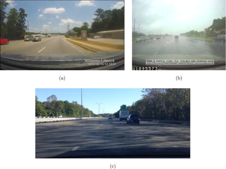
Lane markers with weak signals. (a) An image with high resolution 1604 × 768 captured by the E-PRANCE EP503 vehicle camera.¹³ (b) A frame with resolution 480 × 360 from SHRP2 study.³⁸ (c) An image with high resolution 1604 × 768 but weak lane-marker signal.

In existing literature, it is rare to evaluate lane-marker detection or lane-change event detection using vast naturalistic driving data. In this paper, we report an automated method for lane-change detection in a data set of 490-h long, low-resolution naturalistic driving videos, which was much larger than most testing data sets used in previous literature. Because the goal of our study was to reduce the effort and time required for manually reviewing the naturalistic driving videos offline, with minimal loss of true lane-change events, we tuned the detection method to increase the data reduction rate rather than reduce the false discovery rate, to the extent that most of the lane-change events would be detected.

The main contribution of our work is twofold: (1) we proposed to detect lane-change events by accumulating lane-marker candidates over time, i.e. tackling the problem in the temporal domain, which effectively overcame the difficulty due to low resolution, and (2) the proposed method was tested on a large volume of naturalistic driving videos in low resolution to demonstrate its utility in practical problem solving.

2. Method Overview

Compared to high-resolution videos, low-resolution videos have shorter and narrower lane markers and therefore result in a weaker signal for detection. Conventional methods cannot reliably detect the weak lane markers. Figure 2 shows the lane-marker detection for three types of images using Hough transform and Tomazas’ method,³⁴ which is based on references.^7,24,40 The edges are extracted from the original image by a Sobel operator, and the Hough transform image is derived from the edge image. The highlighted area in the Hough transform image corresponds to the highlighted area in the edge image. The brighter the highlighted area in the Hough transform image, the more obvious the edge. For an artificial image (Fig. 2(a)), Tomazas’ method can easily detect the lane markers. For an image with high-resolution lane markers (Fig. 2(b)), the marked edge was mapped as a bright spot in the Hough transform image, and Tomazas’ method can detect line patterns including the lane markers reasonably well. By contrast, for a low-resolution image from our naturalistic driving videos (Fig. 2(c)), the lane-marker edges are likely not the bright spots in the Hough transform image (see the red circle in Fig. 2(c)). While Tomazas’ method was able to detect long line patterns, such as road curbs far from the car, it completely missed the actual dashed lane marker right under the vehicle.

Fig. 2.

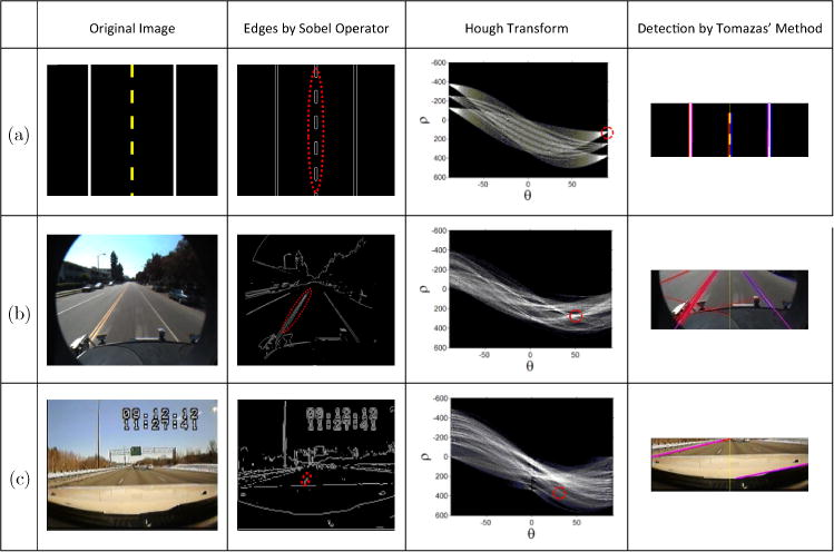
Lane-marker detection for three types of images. (a) An artificial image with ideal lane markers, (b) A high-resolution image with lane markers around 270-pixels long,¹ and (c) A low-resolution image with lane markers around 8-pixels long from our videos. The results of Hough transform and Tomazas’ method³⁴ are demonstrated here. The highlighted edges in the second column correspond to the circle-highlighted spots in the Hough transform images. Line patterns can be detected by finding bright spots in the Hough transform images. The last column demonstrates the detection results of Tomazas’ method,³⁴ which cannot detect low-resolution lane markers in (c).

The fundamental limitation with these conventional lane-marker detection algorithms is that they essentially detect long, strong line patterns (not necessarily solid lines). However, in low-resolution videos such as our data set, the visible lane markers are usually short and thin, due to the strong perspective effect of wide-angle cameras. To overcome the problem, we propose a method to detect weak lane markers by examining a number of consecutive frames. As Fig. 3 shows, the proposed method consists of four steps.

Fig. 3.

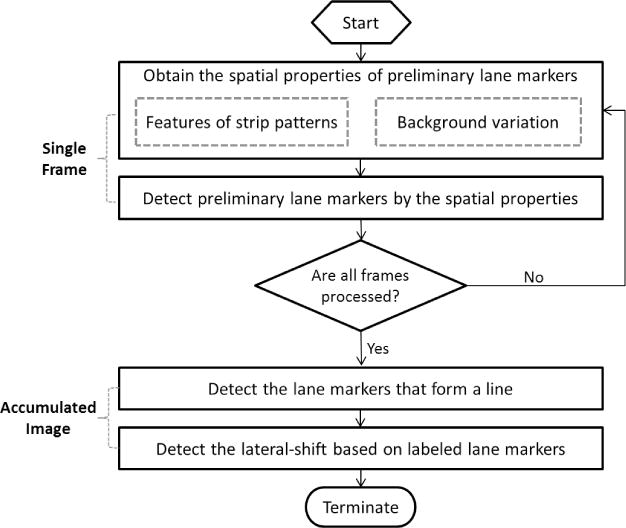
Overview of the proposed lane-change detection framework. The first two steps are completed on each frame independently, and the last two steps are performed on the accumulated image, i.e. the detection lines from all frames in chronological order.

1. Obtain the spatial properties of preliminary lane-marker candidates.

   For each car, we set a detection line 15 pixels above the vehicle hood manually (the red line in Fig. 4(a)). In each video frame, the features of strip patterns (e.g. lane makers) along the detection line is extracted by an adaptive Gaussian-matched filter²⁶ and the background variation is evaluated by a pair of conjugate windows.

2. Detect preliminary lane-marker candidates by the spatial properties.

   The preliminary lane-marker candidates are detected according to the spatial properties of strip patterns, such as the best-matched parameters and the background variation.

3. Detect the lane markers that form a line.

   As Fig. 4(b) shows, an accumulated image is built by stacking up the preliminary lane-marker candidates on the detection lines over time. The real lane markers of the same lane usually form a line in the accumulated image, while the incorrect detection results appear like noise dots. By detecting lane-marker candidates that form continuous lines, the final lane makers are labeled (referred to as labeled lane markers).

4. Detect the lateral-shift based on labeled lane markers.

   If a vehicle maintains its lane position, the labeled lane markers usually form a straight vertical line in the accumulated images. Therefore, the lane-change events can be detected by analyzing the lateral shift of the labeled lane markers.

Fig. 4.

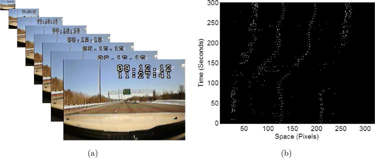
(a) A detection line (the red line) is set across the road and close to the vehicle hood, where the lane markers are most obvious. (b) The accumulated image is obtained by stacking up the preliminary lane-marker candidates on detection lines over time. The value of a pixel in the accumulated image is set to 1 if it is detected as a preliminary lane-marker candidate, and otherwise the pixel value is set to 0 (color online).

3. Obtain the Spatial Properties of Lane-Marker Candidates

The proposed method detects lane markers based on the features of strip patterns as well as the variation of background. A detection line, along which the preliminary lane markers are detected, is placed close to the vehicle hood (Fig. 4(a)). This is because lane markers appear longer, wider, and have more reliable orientation at near distances to the camera. A second-order Gaussian-matched filter is used to extract the features of strip patterns, including the orientation, the width, and the filter response. Additionally, the background variation of a lane marker is another important clue for lane-marker detection, and we evaluated the background variation using a pair of conjugate windows.

3.1. Extracting features of strip patterns using a Gaussian-matched filter

The second-order Gaussian-matched filter (matched filter for short) is effective at detecting strip patterns with orientation, such as retinal blood vessels and layers in retinal optical coherence tomography (OCT) images.^26,49 Similarly, we apply the matched filter to detect lane markers, and accordingly utilize the parameters of the matched filter to represent the features. The model of the matched filter is given by^26,49:

$$f\left(x,y\right)=\frac{1}{\sqrt{2\pi }{\sigma }^{3.5}}\left(x^2-{\sigma }^2\right)e^{-\frac{x^2}{2{\sigma }^2}},\left|x-c\right|\le w/2,$$ (1)

where σ controls the spread of the filter, c is the x position of the center line of the filter window along the y axis, and w is the width of the filter window.

Equation (1) assumes that the orientation of the filter is aligned along the y axis. For lane markers, the orientations are arbitrary. Therefore, one more parameter, θ, is added to describe the orientation, and Eq. (1) is revised as

$$\begin{gathered} f^{\prime }\left(x,y,\theta \right)=-\frac{1}{\sqrt{2\pi }{\sigma }^{3.5}}\left[{\left(\sin \theta ·x-\cos \theta ·y\right)}^2-{\sigma }^2\right]e^{-\frac{{\left(\sin \theta ·x-\cos \theta ·y\right)}^2}{2{\sigma }^2}}, \\ D\left({L^{\prime }}_c\left(x\right),\left(xy\right)\right)\le w/2, \end{gathered}$$ (2)

where $D\left({L^{\prime }}_c,\left(xy\right)\right)$ is used to constrain the distance from the point (x, y) to the center line ${L^{\prime }}_c$, which is defined as sin θ · x − cos θ · y = c.

3.2. Computing the background variation using a pair of conjugate windows

While the matched filter can detect weak lane markers, it is also sensitive to step edges. As Figs. 5(a) and 5(b) demonstrate, the edges of the road and the garage frame may be detected as lane markers. The proposed method eliminates the falsely detected edges, based on an assumption that the background (road surface) of the lane marker is uniform in a local area.

Fig. 5.

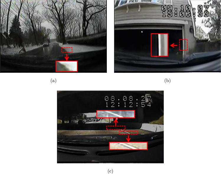
Background of lane-marker candidates. The original areas (marked by dashed lines) are processed to obtain the reflectance (indicated by the inset rectangles, which were magnified for illustration). The step edges in (a) and (b) look like lane markers but the reflectance insets clearly show the lack of background uniformity. (c) The two marked areas along the same lane marker in the same frame appear different due to the shadow; however, they are similar in the reflectance insets because reflectance is invariant to the ambient illumination.

Although the road surface is uniform in local areas, illumination variation may occur within one frame (e.g. shadow) or across different frames, making it difficult to set a universal threshold to determine the uniformity of the background. For instance, the highlighted areas in Figs. 5(a) and 5(b) have different illumination, and the shadow in Fig. 5(c) causes the two local areas in the same frame to be different. According to Retinex theory, reflectance is invariant to the illumination,^20,22,41,42 so our method uses reflectance rather than the raw image to evaluate the background variation. Based on Retinex theory, the reflectance of a window can be derived by

$$R\left(x,y\right)=SQ\left(cx+x,cy+y\right)/I_e,$$ (3)

where (cx; cy) indicates the centers of the window, SQ indicates the lightness of the window, I_e is the environment illumination, which is simply estimated by the average lightness of the brightest 10% pixels in the window, and R (x; y) is the reflectance of the window.

Our method uses a pair of conjugate windows (as shown in the highlighted insets in Fig. 5) to measure the difference between the reflectance on the two sides of the lane marker. The two windows are named the left and right windows, as shown in Fig. 6(b). The difference between the two conjugate windows is computed as follows:

$$D_{cq}=\frac{1}{N}{\displaystyle \sum _{i=-\text{win}}^{\text{win}}{\displaystyle \sum _{j=-\text{win}}^{\text{win}}\left|R_l\left(i,j\right)-R_r\left(i,j\right)\right|}},$$ (4)

where the win is empirically set to 4, the width of the window is $2\ast \text{win}+1=9$, and the number of pixels in each window is $N={\left(2\ast \text{win}+1\right)}^2$.

Fig. 6.

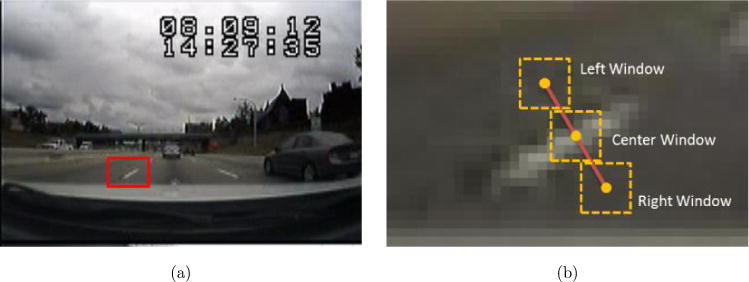
Illustration of conjugate windows. (a) A naturalistic driving image. (b) Magnification of the marked area in (a), with a pair of conjugate windows and a center window. The red line in (b) connects the centers of the left window and the right window, perpendicularly to the direction of the lane marker, and the centers of the window lie on the lane marker (color online).

4. Detect Lane Markers by the Spatial Properties

The proposed method detects preliminary lane-marker candidates using the best-matched parameters of the filter and the background variation. Only the strip patterns with large response peak, reasonable direction and width, and small background variation are considered as final lane markers. Specially, the preliminary lane markers that satisfy the following criteria are preserved:

1. The filter response peak RSP_peak is greater than an empirically set lower bound, RSP_lower = 60.

2. The range of the parameter σ_best, which depends on the width of the lane marker, is set to [0.5,5]. A small range is useful to speed up the computation, while a large range makes the method more robust to lane-change width variation.

3. The range of the best-matched orientation θ_best is empirically set to [30°, 150°], to exclude strip patterns along the horizontal direction. The method can tolerate different ranges of this parameter as far as the horizontal strip patters can be excluded.

4. The background reflectance variation is less than an empirically set upper bound, CJD_upper = 60.

After obtaining the preliminary lane-marker candidates for each frame, we stack up the detection line in chronological order to obtain an accumulated image (Fig. 4(b)). Each row of the accumulated image is a detection line from one frame, with 1 indicating the lane-marker candidate and 0 indicating the nonlane-marker candidate.

5. Detect Lane Markers Forming a Line

In the accumulated image, the true lane markers of the same lane usually form a line (referred to as the lane-marker line), such as the four obvious lines in Fig. 4(b). The direction of the lane-marker line would be almost vertical in the case that the vehicle maintains a steady lane position, while it would deviate from the vertical direction in the case that the vehicle turns. Therefore, the challenge of lane-change detection can be transformed into a line-orientation detection problem.

Since naturalistic driving conditions vary greatly, the accumulated image may have many false lane markers (Fig. 4(b)), which can cause false alarms. The proposed method filters out false lane markers by double checking the preliminary lane markers using an oriented histogram. To obtain the oriented histogram, a circle is centered on the preliminary lane marker. For each direction of 1°, 2°, 3°, … 180°, an oriented stripe across the center of the circle (the area marked by the red rectangle shown in Fig. 7) is defined, and the number of preliminary lane markers in the stripe is counted. The diameter of the circle is set equal to the lane width w_l, and the width of the stripe is set to $w_l\ast 0.15$. The oriented histogram is defined as an array of preliminary lane-marker counts obtained from the 180 evenly distributed stripes around the center.

Fig. 7.

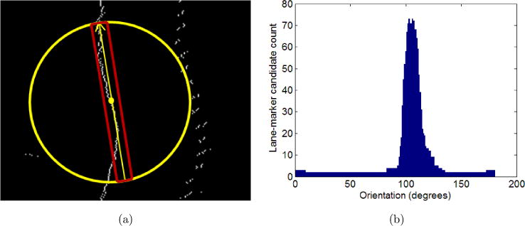
Illustration of an oriented stripe and an oriented histogram. (a) An oriented stipe is an area crossing the center of a circle, with two long sides equidistant from a diameter of the circle, and the other two sides on the boundary of the circle. (b) The oriented histogram, i.e. lane-marker candidate count, obtained from 180 evenly distributed stripes around the center of the yellow circle in Fig. (a) (color online).

The oriented histogram typically has a peak along the orientation of the lane-marker line (Fig. 7 (b)). To check if the distribution of preliminary lane markers forms a lane-marker line, the proposed method uses a threshold P_lower:

$$P_{\text{lower}}=t·{\displaystyle \sum _{i=1}^{N}h\left(i\right)/N},$$ (5)

where h(i) indicates the value of the ith histogram bin, t is a constant value, empirically set to 4.

If the highest peak in the histogram is above the threshold P_lower, the candidate is regarded as a final lane marker, and also its orientation is assigned as the orientation of the histogram peak. Otherwise, the lane-marker candidate is removed. The labeled lane markers are later used to compute the lateral shift of the vehicle.

6. Detect Lane-Change Events

Lane-change events were detected by the lateral variation of lane markers. In the accumulated image, since a vertical lane-marker line implies no vehicle lateral shift, we only considered lane markers with orientation in [30°, 80°] and [100°, 150°]. At a small scale, the lane-marker line is approximately a straight line, which can be modeled using the position and the orientation of a lane marker, but it may not be true at a larger scale. Therefore, our method analyzed the lane-marker line in a segment-wise manner.²⁹

As Fig. 8 shows, given a labeled lane marker P, the line L_lm passing through it is

$$\sin \left(\theta \right)·x-\cos \left(\theta \right)·y=\sin \left(\theta \right)·x_0-\cos \left(\theta \right)·y_0,$$ (6)

where (x₀, y₀) and θ are the coordinates and the orientation of the lane marker P (obtained from the oriented histogram).

Fig. 8.

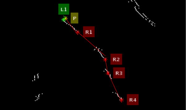
Detection of the rightmost and leftmost lane markers along a lane-marker line. The line passing through a lane marker is modeled using its coordinate and orientation.

All the lane markers (x, y), which satisfy the criteria defined by Eqs. (7) and (8), are found.

$$D\left(\left(x,y\right),\left(x_0{y}_0\right)\right)\le w_l/2,$$ (7)

where D((x, y), (x₀, y₀)) indicates the distance from the lane marker at (x, y) to (x₀, y₀)

$$D\left(L_{\text{lm}},\left(x,y\right)\right)\ge w_l\ast 0.075,$$ (8)

where D(L_lm, (xy)) indicates the distance from the lane marker at (x, y) to the line L_lm

Among all the surrounding lane markers satisfying Eqs. (7) and (8), assume R₁ is the one with the largest horizontal coordinate, i.e. the rightmost. The line passing through R₁ can also be modeled according to its coordinate and orientation, and then a new rightmost candidate R₂ can be found using R₁ as reference. This process is repeated as long as the distance between the latest rightmost lane marker and P is less than 2w_l. Such a threshold is set to avoid analyses over a too long range, which may complicate data involved. In Fig. 8, the final rightmost lane-marker candidate is R₄. The leftmost lane marker can be found in a similar way.

A lane-change event is detected if the rightmost and the leftmost lane markers meet the two criteria: (1) The horizontal distance (lateral shift) between the rightmost and the leftmost lane markers is larger than 0.8w_l. In other words, only the events with obvious lateral shift in a local area are considered as lane-change events. (2) The rightmost and the leftmost lane markers are on two opposite sides of the middle line of the accumulated image. This requires that the lane marker should run across the camera center.

7. Experiments

7.1. Experimental setup

The test data consisted of 490 h of naturalistic driving video collected by Ott et al. from 63 cognitively impaired drivers in a previous study.^2,33 Cameras were installed in the drivers’ cars, and continuous video recording was collected over a two-week period. Cameras captured front, sides, and rear views (four channels). Video from the cameras was automatically saved to a portable digital video-recording device that was placed under the passenger seat. Participants were instructed to drive in their typical environment and routine. The resolution of each video channel was 352 × 240 and lane markers, which are from the front-view channel, were typically no wider than 3 pixels.

Many of the driving videos were not reviewed manually in Ott’s clinic studies, due to the large amount of labor and time required. The proposed lane-change detection technique was used for data reduction. The experimental environment is an Intel (R) Core (TM) i7-4790 CPU @ 3.6 GHz, Windows 7, and Microsoft Visual Studio 2008 C#. Our goals were (1) detecting lane-change events with minimum missed detections; and (2) reducing the quantity of data to an acceptable level for manual review. Therefore, unlike previous papers,^1,45 this experiment did not focus on the evaluation of lane-marker detection for each frame. Instead, the sensitivity of lane-change detection, the false discovery rate, and the data reduction rate were the main outcome measures.

To evaluate the sensitivity of the proposed method, a 10-h subset from the 490-h data set was arbitrarily selected and 154 real lane-change events were manually labeled. The labeled lane-change events served as the ground truth. The average duration of a lane-change event is 9 s. Compared to previous studies^1,45 which usually had less than 2 h of manually coded videos, our test videos contained much more complicated road conditions. The remaining 480-h videos were processed by the proposed method to detect the lane-change events. A bootstrapping method was used to determine whether the results from the 10 h of test videos could be generalized to the other 480-h data set. Finally, we summarized the causes for incorrectly detected lane-change events.

7.2. Results

The proposed method is rather effcient, since this method is designed to process only one line for each frame. Our program needs around 5 min to process a 1-h video. For the 10 h of coded video, the proposed method correctly detected 146 of the 154 labeled events, and falsely marked 111 nonlane-change events. In other words, the method achieved a sensitivity of 94.8% (146/154) with a false discovery rate of 43.2% (111/257). Based on the total length of lane-change event clips, the data reduction rate was 93.6%. Given such a high data reduction rate, the 43.2% of additional video-reviewing effort due to false discoveries was acceptable, as it was only 38.6 min out of 10 h. The eight missed lane-change events were respectively due lane-marker missing (one event), image sensor smear from the sun (one event), windshield wiper occlusion (two events), spots on windshield (two events), and slow lateral shift (two events). Reasons for these missed events are elaborated below.

1. Lane-marker missing: Figs. 9(a)–9(c) illustrate three frames in chronological order of such a missed lane-change event. The lane marker could be seen at the beginning and the end of the lane change, but disappeared for most of time of the lane change (Fig. 9(b)). Our method failed to detect the lateral shift of the lane marker as a lane-change event.

2. Image sensor smear: The image sensor smear due to the sun was a white line crossing the image vertically. Since the smear was brighter than the real lane marker, it was identified as a lane marker instead. When a true lane-change event happened, the smear line maintained its horizontal position as Figs. 9(d)–9(f) show, and therefore our method mistakenly determined the lane position was steady.

3. Windshield wiper occlusion: The windshield wiper occluded the view so that the proposed method failed to detect the lane marker. Figure 9(g) illustrates a frame of a missed lane-change event due to windshield wiper occlusion.

4. Spots on windshield: in one subject’s video, a white spot on windshield happened to be on the detection line, as shown in Fig. 9(h). The spot resulted in a steady lane-marker line in the accumulated image, and therefore it was assumed that the vehicle kept the lane position.

5. Slow lateral shift: The lateral shift was so slow that it took a much longer time than was typical (and therefore many more frames) to finish the lane-change event. Since our method was set to detect lane change within 320 frames, it failed to find such slow lane-change events.

Fig. 9.

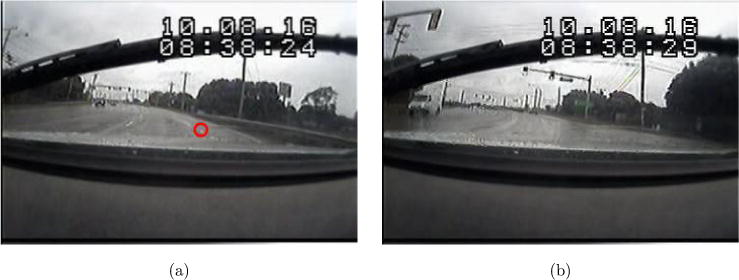
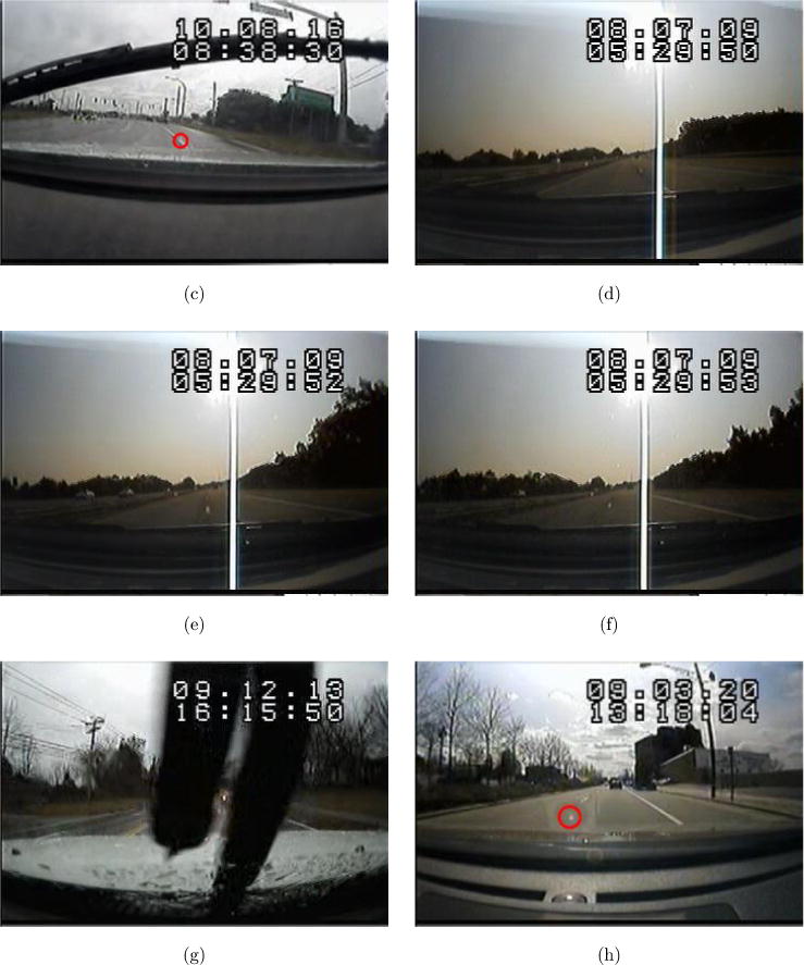
Examples of missed lane-change events. (a–c) Three frames in chronological order of a missed lane-change event due to lane marker missing during the lane change. (d–f) Three frames in chronological order of a missed lane-change event due to sensor smear. (g) A frame of a missed lane-change events due to windshield wiper occlusion. (h) A frame of a missed lane-change event due to a spot on windshield.

For the 480 h of video, 4971 lane-change events were flagged by our method. All of them were manually reviewed, and the results indicated that 2370 flagged events (47.7%) were real lane changes and the other 2601 (52.3%) were not. In other words, the false discovery rate was 52.3%, and the data reduction rate was 97.4%. Sensitivity was unknown as we could not practically code all 480 h of video.

According to our review, the false positive lane-change events were mainly due to three causes: lane variation (1409 events), other bright patterns (697 events), and incorrect lane-marker detection (495 events).

1. Lane variation: Road curvature, road division, merging roads, and lane width change are common lane variation. Figures 10(a) and 10(b) illustrate two frames of a falsely detected event due to lane width change. The right lane marker did shift to the right, but that was because the car moved to the center of a widening lane.

2. Bright patterns: Some bright patterns, such as the sensor smears and white posts in the light color, were incorrectly identified as lane markers and shifted laterally when the vehicle made a turn. Figures 10(c)–10(e) show three frames in chronological order of a falsely detected event due to smear. The smear moved from left to right relative to the camera, resulting in a falsely detected event.

3. False lane-marker detection: Due to environment changes and noises, the proposed method sometimes could not detect lane markers correctly, and further resulted in falsely detected events.

Fig. 10.

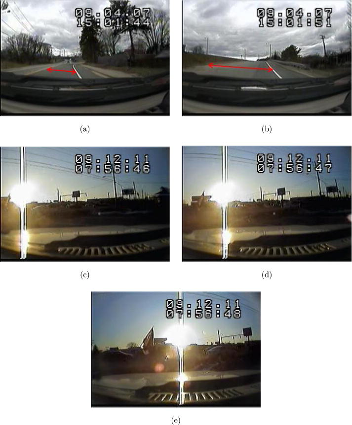
Examples of false positive events. (a) and (b) are two frames in chronological order showing a falsely detected event due to lane width change. The car drove on the right lane maker first, and then moved to the lane center when the lane became wider. (c)–(e) Three frames in chronological order of a falsely detected events due to smear. The smear moved from left to right relatively to the camera when the car turned, resulting in a falsely detected event.

To test if the false discovery rate of the 480 h of data (52.3%) was similar to that of the 10-h coded sample (43.2%), we used a bootstrapping procedure in which we randomly selected 10-h samples from the 480-h data set 10,000 times and then calculated the distribution of the false discovery rates, as shown in Fig. 11. We found that the false discovery rate (43.2%) of the 10-h fully coded data set was within the 95% confidence interval ([39.2%, 64.3%]). Therefore, the 10-h coded data set can be considered as a reasonable approximation of the whole 490-h data set, as far as lane-change detection is concerned. This finding might suggest that the sensitivity (94.8%) based on the 10-h data set is also representative of the 490-h data set. In general, when a method is tuned for detection, an increase in false discovery rate is associated with an increase in sensitivity. As the 10-h false discovery was at the lower side of the 480-h false discovery rate distribution, it could be speculated that the actual sensitivity of the 480-h data set might be higher than the sensitivity of the 10-h fully coded data set.

Fig. 11.

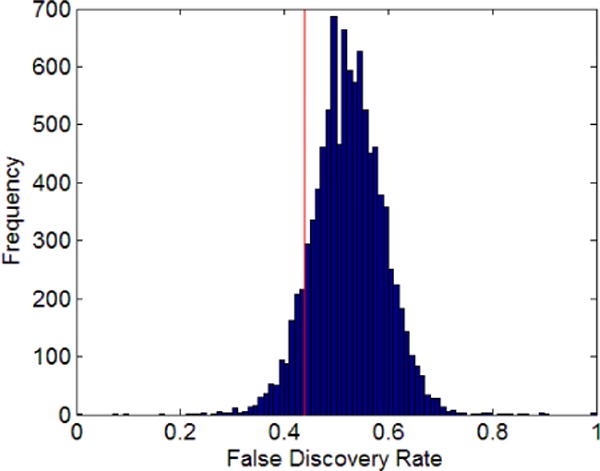
Distribution of false discovery rate for the 10,000 10-h samples from the 480-h data set. The 95% confidence interval of the false discovery distribution is [39.2%, 64.3%], and the mean is 52.4%. The red line marks the false discovery rate (43.2%) of 10-h coded videos (color online).

We have also tested some existing lane detection methods on the naturalistic driving videos.^7,24,40 None of the methods can detect the low-resolution lane markers in our videos. One of the methods we tested is shown in Fig. 2. We can see that it failed completely for our images. Because they cannot detect lane markers, it is not fair conduct lane-change detection comparison in this paper.

In addition, we have also tested the proposed method on a recently released data set,³⁵ which has totally 500-min recording involving six drivers. The videos of this data set are in higher resolution than our naturalistic driving data set. Overall, the data reduction rate is 92% and the sensitivity of lane-change events is 97.0%. Note: 20 incorrectly labeled ground truth events were excluded after visual examination. For example, the duration of the second video of subject D1 is 638 s, but two ground truth events are labeled at 646 and 656 s. Table 1 shows the detection results, which are similar for all drivers except for D5. The missed detection for D5 was mainly due to the window shield occlusion. In general, the sensitivity of lane-change events on this data set is higher than that on our naturalistic driving data set. That is because the videos of this data set have higher resolution and the weather conditions were mostly better than in our videos.

Table 1.

Sensitivity of lane-change events on the public data set.³⁵

Driver	D1	D2	D3	D4	D5	D6	Average
Sensitivity(%)	100	100	98.1	96.6	84.8	98.5	97.0
Number of ground truth	79	75	95	50	44	63	73

8. Discussion and Conclusions

We have proposed a lane-change detection method based on temporally accumulated images. Our method is different from existing methods in that lane markers are detected over time rather than in a single frame, which overcame the difficulty due to low-resolution and possible interferences, such as occlusion within a single frame. This is critical for processing low-resolution images, where many existing methods failed.

We set the parameters of the method empirically, instead of using a machine learning procedure to tune the parameters. Systematically fine-tuning parameters could increase the method’s performance. However, despite using empirical parameters, the method was not sensitive to the complexity of the images involving diversified driving conditions. Being able to successfully process an enormous amount of driving videos recorded from 63 people in their own environments demonstrated the robustness of the proposed method.

Although the image resolution in other applications is not always low, situations in which lane markers are difficult to discern are not rare in naturalistic driving videos. The causes include faded markers, bad weather, low illumination, etc. Fundamentally, the challenge is how to detect the weak signals of lane markers in those conditions. Because of the optical perspective effect, the width of lane markers in images shrinks with distance, and the perspective effect quickly increases with the field of view of the camera. In naturalistic conditions, the lane markers in the distance can easily be buried in other image patterns. Focusing only on lane markers at close distances, where lane markers are relatively easier to detect, and tracking them over time, i.e. temporal processing of lane markers, can be a sound strategy to resolve the weak-signal problem.

Data reduction of naturalistic driving videos is not only needed for driving safety research, it is also highly demanded in machine learning or deep learning work used in ADAS and self-driving applications. This type of work requires enormous natural driving data, hand coded by human observers. Without data reduction, the hand coding burden can be prohibitively high. A reduction rate of 97% as we achieved in this study can be appealing. We envision that methods of lane-change detection from naturalistic driving videos can be useful to train machines to make lane changes like humans. Similar efforts have been initiated to train machines to steer a cars using deep learning neural networks.³

Biographies

Brian Ott received his Doctor of Medicine degree from Jefferson Medical College in Philadelphia in 1979. He is currently a Professor in the Department of Neurology, in the Alpert Medical School of Brown University in Providence, Rhode Island, as well as Adjunct Professor in the School of Pharmacy at the University of Rhode Island. At Rhode Island Hospital in Providence, he serves as the director of the Alzheimer’s Disease and Memory Disorders Center.

His primary research interest focuses on the effects of aging and dementia on driving in the elderly. His work is primarily funded by the National Institutes of Health, National Institute on Aging, where he has received continuous funding since 2001, including a longitudinal study of cognition and road test performance in drivers with Alzheimer’s disease, and a more recent project involving naturalistic assessment of driving in cognitively impaired elders. He has also recently begun a clinical trial funded by the Alzheimer’s Association examining a video feedback intervention for the safety of cognitively impaired older drivers.

Shuhang Wang received the B.S. degree in computer science and engineering from North-western Polytechnical University, Xian, China, in 2009, and the Ph.D. degree in computer science and engineering from Beihang University, Beijing, China, in 2014.

He is currently a postdoctoral research fellow at Schepens Eye Research Institute, Harvard Medical School. His current research interests are image processing, computer vision, driving behavior, and artificial intelligence.

Gang Luo received his Ph.D. degree from Chongqing University, China in 1997. In 2002, he finished his postdoctoral fellow training at Harvard Medical School. He is currently an Associate Professor at The Schepens Eye Research Institute, Harvard Medical School. His primary research interests include basic vision science, and technology related to driving assessment, driving assistance system, low vision, and mobile vision care.

References

- 1.Aly M. Real time detection of lane markers in urban streets. 2008 IEEE Intelligent Vehicles Symp. 2008:7–12. [Google Scholar]
- 2.Bixby K, Davis JD, Ott BR. Comparing caregiver and clinician predictions of fitness to drive in people with Alzheimer’s disease. Am J Occup Ther. 2015;69(3):6903270030p1–6903270030p7. doi: 10.5014/ajot.2015.013631. [DOI] [PMC free article] [PubMed] [Google Scholar]
- 3.Bojarski M, et al. End to end learning for self-driving cars. 2016 Apr; [Google Scholar]
- 4.Borkar A, Hayes M, Smith MT. A novel lane detection system with effcient ground truth generation. IEEE Trans Intell Transp Syst. 2012;13(1):365–374. [Google Scholar]
- 5.Bowers A, Peli E, Elgin J, McGwin G, Owsley C. On-road driving with moderate visual field loss. Optom Vis Sci. 2005;82(8):657–667. doi: 10.1097/01.opx.0000175558.33268.b5. [DOI] [PubMed] [Google Scholar]
- 6.Bowers AR, Mandel AJ, Goldstein RB, Peli E. Driving with hemianopia, II: Lane position and steering in a driving simulator. Invest Ophthalmol Vis Sci. 2010;51(12):6605–6613. doi: 10.1167/iovs.10-5310. [DOI] [PMC free article] [PubMed] [Google Scholar]
- 7.Canny J. A computational approach to edge detection. IEEE Trans Pattern Anal Mach Intell. 1986;8(6):679–698. [PubMed] [Google Scholar]
- 8.Carney C, McGehee D, Harland K, Weiss M, Raby M. Using naturalistic driving data to assess the prevalence of environmental factors and driver behaviors in teen driver crashes. Available at http://www.cartalk.com/
- 9.Classen S, Shechtman O, Awadzi KD, Joo Y, Lanford DN. Traffic violations versus driving errors of older adults: Informing clinical practice. Am J Occup Ther. 2010;64(2):233–241. doi: 10.5014/ajot.64.2.233. [DOI] [PubMed] [Google Scholar]
- 10.Dai J, Teng J, Bai X, Shen Z, Xuan D. Mobile phone based drunk driving detection. Proc 4th Int ICST Conf Pervasive Computing Technologies for Healthcare. 2010:1–8. [Google Scholar]
- 11.Davis JD, et al. Road test and naturalistic driving performance in healthy and cognitively impaired older adults: Does environment matter? J Am Geriatr Soc. 2012;60(11):2056–2062. doi: 10.1111/j.1532-5415.2012.04206.x. [DOI] [PMC free article] [PubMed] [Google Scholar]
- 12.Dingus TA, et al. The 100-Car naturalistic driving study phase II — Results of the 100-Car field experiment. 2016 [Google Scholar]
- 13.E-PRANCE® EP503 Dash Cam Super HD 1296P Car DVR Camera.
- 14.Gaikwad V, Lokhande S. Lane departure identification for advanced driver assistance. IEEE Trans Intell Transp Syst. 2015;16(2):910–918. [Google Scholar]
- 15.He J. Lane Keeping Under Cognitive Distractions-Performance and Mechanisms. University of Illinois; Urbana-Champaign: 2012. [Google Scholar]
- 16.Hillel AB, Lerner R, Levi D, Raz G. Recent progress in road and lane detection: A survey. Mach Vis Appl. 2014;25(3):727–745. [Google Scholar]
- 17.Jiang R, Klette R, Vaudrey T, Wang S. Corridor detection and tracking for vision-based driver assistance system. Int J Pattern Recognit Artif Intell. 2011;25(2):253–272. [Google Scholar]
- 18.Johnson DA, Trivedi MM. Driving style recognition using a smartphone as a sensor platform. IEEE Conf Intell Transp Syst Proceedings, ITSC. 2011:1609–1615. [Google Scholar]
- 19.Kim Z. Robust lane detection and tracking in challenging scenarios. IEEE Trans Intell Transp Syst. 2008;9(1):16–26. [Google Scholar]
- 20.Land EH, McCann JJ. Lightness and retinex theory. J Opt Soc Am. 1971;61(1):1–11. doi: 10.1364/josa.61.000001. [DOI] [PubMed] [Google Scholar]
- 21.Lee SE, Olsen ECB, Wierwille WW. A comprehensive examination of naturalistic lane-changes. 2004 [Google Scholar]
- 22.Li B, Wang S, Geng Y. Image enhancement based on Retinex and lightness decomposition. 2011 18th IEEE Int Conf Image Processing. 2011:3417–3420. [Google Scholar]
- 23.Li W, Guan Y, Chen L, Sun L. Millimeter-wave radar and machine vision-based lane recognition. Int J Pattern Recogn Artif Intell. 2017:1850015. [Google Scholar]
- 24.Lim KH, Ang LM, Seng KP, Chin SW. Lane-vehicle detection and tracking; Proc Int Multiconference of Engineers and Computer Scientists 2009 Vol II IMECS 2009; Hong Kong. 2009. [Google Scholar]
- 25.Luo G, Peli E. Methods for automated identification of informative behaviors in natural bioptic driving. IEEE Trans Biomed Eng. 2012;59(6):1780–1786. doi: 10.1109/TBME.2012.2191406. [DOI] [PMC free article] [PubMed] [Google Scholar]
- 26.Luo G, Chutatape O, Krishnan SM. Detection and measurement of retinal vessels in fundus images using amplitude modified second-order Gaussian filter. IEEE Trans Biomed Eng. 2002;49(2):168–172. doi: 10.1109/10.979356. [DOI] [PubMed] [Google Scholar]
- 27.Mattes S. The lane-change-task as a tool for driver distraction evaluation. Qual Work Prod Enterp Futur. 2003:57–60. [Google Scholar]
- 28.McCall JC, Trivedi MM. Video-based lane estimation and tracking for driver assistance: Survey, system, and evaluation. IEEE Trans Intell Transp Syst. 2006;7(1):20–37. [Google Scholar]
- 29.Montgomery DC, Peck EA, Vining GG. Introduction to Linear Regression Analysis. 2015 [Google Scholar]
- 30.Neale VL, Dingus TA, Klauer SG, Goodman M. An overview of the 100-car naturalistic study and findings. 19th Enhanced Safety Vehicles Conf. 2005:1–10. [Google Scholar]
- 31.Neale VL, Klauer SG, Knipling RR, Dingus TA, Holbrook GT, Petersen A. The 100 car naturalistic driving study: Phase 1- experimental design. 2002 [Google Scholar]
- 32.Nobukawa K, Bao S, LeBlanc DJ, Zhao D, Peng H, Pan CS. Gap acceptance during lane changes by large-truck drivers — An image-based analysis. IEEE Trans Intell Transp Syst. 2016;17(3):772–781. doi: 10.1109/TITS.2015.2482821. [DOI] [PMC free article] [PubMed] [Google Scholar]
- 33.Ott BR, Papandonatos GD, Davis JD, Barco PP. Naturalistic validation of an on-road driving test of older drivers. Hum Factors J Hum Factors Ergon Soc. 2012;54(4):663–674. doi: 10.1177/0018720811435235. [DOI] [PMC free article] [PubMed] [Google Scholar]
- 34.Project implements a basic realtime lane and vehicle tracking using OpenCV. 2015 https://github.com/tomazas/opencv-lane-vehicle-track.
- 35.Romera E, Bergasa LM, Arroyo R. Need data for driver behaviour analysis? Presenting the public UAH-DriveSet. IEEE 19th Int Conf on Intelligent Transportation Systems (ITSC) 2016:387–392. [Google Scholar]
- 36.Satzoda RK, Trivedi MM. Effcient lane and vehicle detection with integrated synergies (ELVIS) 2014 IEEE Conf Computer Vision and Pattern Recognition Workshops. 2014;1:708–713. [Google Scholar]
- 37.Satzoda RK, Trivedi MM. Vision-based lane analysis: Exploration of issues and approaches for embedded realization. IEEE Comput Soc Conf Comput Vis Pattern Recognit Work. 2013:604–609. [Google Scholar]
- 38.The Second Strategic Highway Research Program. Available at http://www.trb.org/StrategicHighwayResearchProgram2SHRP2/Blank2.aspx.
- 39.Sehestedt S, Kodagoda S. Effcient lane detection and tracking in urban environments. EMCR. 2007:1–6. [Google Scholar]
- 40.Viola P, Jones M. Rapid object detection using a boosted cascade of simple features. Proc 2001 IEEE Comput Soc Conf on Computer Vision and Pattern Recognition (CVPR 2001) 2001;1:I–I. [Google Scholar]
- 41.Wang S, Luo G. Naturalness preserved image enhancement using a priori multi-layer lightness statistics. IEEE Trans Image Process. 2017 doi: 10.1109/TIP.2017.2771449. [DOI] [PMC free article] [PubMed] [Google Scholar]
- 42.Wang S, Zheng J, Hu H, Li B. Naturalness preserved enhancement algorithm for non-uniform illumination images. IEEE Trans Image Process. 2013;22(9):3538–3548. doi: 10.1109/TIP.2013.2261309. [DOI] [PubMed] [Google Scholar]
- 43.West SK, et al. Older drivers and failure to stop at red lights. Journals Gerontol— Ser A Biol Sci Med Sci. 2010;65(2):179–183. doi: 10.1093/gerona/glp136. [DOI] [PMC free article] [PubMed] [Google Scholar]
- 44.World Health Organization. Global status report on road safety 2015. 2015 [Online]. Available: http://www.who.int/violence_injury_prevention/road_safety_status/2015/en/
- 45.Yoo H, Yang U, Sohn K. Gradient-enhancing conversion for illumination-robust lane detection. IEEE Trans Intell Transp Syst. 2013;14(3):1083–1094. [Google Scholar]
- 46.Young K, Regan M. Driver distraction: A review of the literature. Distracted Driv. 2007:379–405. [Google Scholar]
- 47.Young KL, Lee JD, Regan MA. Driver Distraction: Theory, Effects, and Mitigation. CRC Press; 2008. [Google Scholar]
- 48.Young KL, Lenné MG, Williamson AR. Sensitivity of the lane change test as a measure of in-vehicle system demand. Appl Ergon. 2011;42(4):611–618. doi: 10.1016/j.apergo.2010.06.020. [DOI] [PubMed] [Google Scholar]
- 49.Yu D, et al. Computer-aided analyses of mouse retinal OCT images — an actual application report. Ophthalmic Physiol Opt. 2015;35(4):442–449. doi: 10.1111/opo.12213. [DOI] [PMC free article] [PubMed] [Google Scholar]