Enumerating consistent sub-graphs of directed acyclic graphs: an insight into biomedical ontologies

Abstract

Motivation

Modern problems of concept annotation associate an object of interest (gene, individual, text document) with a set of interrelated textual descriptors (functions, diseases, topics), often organized in concept hierarchies or ontologies. Most ontology can be seen as directed acyclic graphs (DAGs), where nodes represent concepts and edges represent relational ties between these concepts. Given an ontology graph, each object can only be annotated by a consistent sub-graph; that is, a sub-graph such that if an object is annotated by a particular concept, it must also be annotated by all other concepts that generalize it. Ontologies therefore provide a compact representation of a large space of possible consistent sub-graphs; however, until now we have not been aware of a practical algorithm that can enumerate such annotation spaces for a given ontology.

Results

We propose an algorithm for enumerating consistent sub-graphs of DAGs. The algorithm recursively partitions the graph into strictly smaller graphs until the resulting graph becomes a rooted tree (forest), for which a linear-time solution is computed. It then combines the tallies from graphs created in the recursion to obtain the final count. We prove the correctness of this algorithm, propose several practical accelerations, evaluate it on random graphs and then apply it to characterize four major biomedical ontologies. We believe this work provides valuable insights into the complexity of concept annotation spaces and its potential influence on the predictability of ontological annotation.

Availability and implementation

https://github.com/shawn-peng/counting-consistent-sub-DAG

Supplementary information

Supplementary data are available at Bioinformatics online.

1 Introduction

Ontologies have become a common means of concept annotation in computational biology and related fields (Robinson and Bauer, 2011). A protein’s molecular function (Ashburner et al., 2000), an effect of a genetic variant (Vihinen, 2014), or a patient’s diagnosis (Robinson and Mundlos, 2010) are typical examples wherein biomedical entities such as macromolecules, mutations, or individuals are associated with sets of mutually dependent descriptors. The dependencies between these descriptors are often hierarchical, leading to the use of directed acyclic graphs (DAGs) as concept space representations.

A DAG is a pair (V, E), where V is a set of vertices (nodes) and E is a set of directed edges (links) between vertices such that no cycles can be formed. Each vertex in the graph is associated with a unique concept (term, description) and each edge is associated with a particular type of relational tie. For example, when annotating proteins as biomedical entities using the Gene Ontology (GO) graph (Ashburner et al., 2000), the terms ‘nucleic acid binding’ and ‘DNA binding’ are linked by edges of the type is-a asserting that DNA binding is a more specific form of nucleic acid binding. Other types of relational ties include part-of, regulates and so on.

A typical biomedical entity is associated with a set of terms determined experimentally such as through a molecular assay or a diagnostic procedure. A protein, for example, may be assigned terms ‘DNA binding’ and ‘RNA binding’, neither of which is a generalization of the other. To avoid annotation inconsistencies, this protein must also be annotated by the terms such as ‘nucleic acid binding’ and all others that generalize either of the experimentally determined terms. More broadly, this implies that a biomedical object can only be annotated by a set of terms that respect the hierarchy––a consistent sub-graph of the ontology. Unfortunately, (manual) experimental annotation is resource-intensive and often incomplete (Poux and Gaudet, 2017), giving rise to an entire field of computational prediction (Jiang et al., 2016; Radivojac et al., 2013).

The development of computational prediction methods presents its own challenges. Although it can be performed by building a separate binary classifier for each concept in the ontology, this approach is currently competitive only for specialized ranking tasks; e.g. disease-gene prioritization (Moreau and Tranchevent, 2012), since it does not exploit relationships between the terms. On the other hand, a more complete characterization is via learning structured outputs (Sokolov and Ben-Hur, 2010) in which a method takes an object (e.g. a protein) and is asked to provide the totality of concepts with which this object might be associated (i.e. a consistent sub-graph). However, the structured-output formulation generally falls under the extreme classification umbrella because the size of the output space is often exceedingly large. This poses problems in measuring similarity between annotations, evaluating accuracy of classification models and optimization when solving the ‘argmax problem’ (Clark and Radivojac, 2013; Joachims et al., 2009; Joslyn et al., 2004; Lord et al., 2003; Pesquita, 2017; Verspoor et al., 2006).

We identify now what we believe is an open problem in computational biology and computer science; that is, efficiently determining the exact number of consistent sub-graphs in a given ontology. This problem has a linear-time solution for rooted trees (Ruskey, 1981), but to our knowledge no such algorithm exists for DAGs. This paper therefore proposes a practical solution to this enumeration problem, proves its correctness, analyzes run-time complexity and introduces various computational speedups. Using this new approach, we analyze four often-used ontologies from the biomedical domain and explore the space of possible annotations. We believe that the algorithms, software and analysis carried out in this work will lead to better insights into concept annotation spaces and facilitate ontology quality assurance.

2 A motivating example

A growing number of concept annotation problems are formulated as the manual or computational assignment of a set of mutually related textual descriptors to some objects of interest. One of such problems is the computational prediction of protein function (Friedberg and Radivojac, 2017), which can be broadly operationalized as follows:

Given: (i) an amino acid sequence with auxiliary data such as structure, expression, interactions, etc. of a protein p with unknown or incomplete function; (ii) training data that includes sequences, structures, or systems data corresponding to a (large) set of proteins, some of which have their true biological functions available; (iii) a GO; i.e. a concept hierarchy used to represent biological functions of proteins in a structured and easy-to-compute-on form.

Objective: provide a set of GO terms that are most likely to be the true (experimental) annotation of p.

The objects of interest here are proteins and the set of textual descriptors of protein function is given by GO––an ontology with a DAG structure where each node represents a textual descriptor and each edge represents a particular type of a relational tie between two descriptors (Ashburner et al., 2000).

An example of such an annotation is shown in Figure 1, where eight terms from the molecular function domain have been assigned to this protein. Due to the hierarchical organization of GO, both the set of experimentally determined terms and the set of computationally predicted terms must respect this hierarchy. As shown in this example, the annotation by the term ‘DNA binding’, implies the annotation by all the other GO terms that conceptually generalize it; e.g. ‘nucleic acid binding’, ‘binding’, etc. Similarly, ‘sequence-specific DNA binding TF activity’ further adds ‘nucleic acid binding TF activity’ to its annotation graph. Typically, the ontology used to represent the annotation space of proteins contains thousands to tens of thousands of terms, whereas the true annotation of a protein consists of tens to at most hundreds of terms. Because the task of a prediction algorithm is to find the most likely annotation, it must devise an efficient procedure to search through the space of all possible annotations.

Fig. 1.

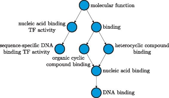
The functional annotation (September 2014) of the friend leukemia integration 1 transcription factor isoform 1 [FLI1; Homo sapiens] (RefSeq ID: NP_002008.2) with experimental evidence codes (including TAS and IC) as a consistent sub-graph of the Molecular Function ontology. The arrows in this graph indicate an is-a relationship and are drawn in the reverse direction

Most biomedical ontologies have grown over the years to contain a large number of terms. Computationally selecting a single ‘winning’ annotation; i.e. a set of terms, or providing a short list of most likely annotations, is a significant challenge (Joachims et al., 2009; Sokolov and Ben-Hur, 2010). This prediction problem belongs to a so-called extreme classification scenario because the number of possible (discrete) annotations the algorithm must consider is astronomically large. In fact, we noticed that it is not possible to give an exact number of annotations available for a protein, even when the ontology is restricted to a fixed low depth. Therefore, an answer to a simple question ‘What is the number of possible GO annotations a protein can be assigned?’ requires the development of a practical counting algorithm. The resulting counts can, in turn, give insight into the nature and the difficulty of the computational function annotation of biological macromolecules (Reasonable approximations can be provided by calculating the lower and upper bounds, as we have done later in Section 6. Neither of those, however, provides a full intellectual satisfaction when an exact count can be computed).

It is important to mention that the annotation of biological macromolecules is one of the most interesting examples of concept annotation, primarily because of its biomedical significance but also because of the sizes and the complexity of the available ontologies. Similar situations, however, arise beyond computational biology, as in the fields of text mining (Grosshans et al., 2014) and computer vision (Movshovitz-Attias et al., 2015).

3 Preliminaries

3.1 Basic concepts and notation

Let $\mathcal{G}=(V,E)$ be a directed graph, where V is a set of vertices representing concepts and $E\subseteq V\times V$ is a collection of ordered pairs (u, v) representing directional relationships, $u\to v$, between two concepts. A sequence of vertices $u_1,u_2,\dots ,u_k$ is called a walk if $(u_i,u_{i+1})\in E$ for $i=1,2,\dots ,k-1$. A walk of distinct vertices except for the identical starting and ending vertices is called a cycle. A directed graph that does not contain cycles is referred to as DAG.

Given two vertices $u,v\in V$ in a DAG, u is said to be an ancestor of v and v is said to be a descendant of u if there exists a walk from u to v. We denote a set of all ancestors of v as $\mathcal{A}\left(v\right)$ and a set of all descendants of u as $\mathcal{D}\left(u\right)$. We next define ${\mathcal{A}}^{+}\left(v\right)=\left\{v\right\}\cup \mathcal{A}\left(v\right)$ as the set of extended ancestors of v and ${\mathcal{D}}^{+}\left(u\right)=\left\{u\right\}\cup \mathcal{D}\left(u\right)$ as the set of extended descendants of u. Finally, if $(u,v)\in E$, the vertex u is said to be a parent of v, whereas v is said to be a child of u. We denote the set of all parents of v as $\mathcal{P}\left(v\right)$ and the set of all children of u as $\mathcal{C}\left(u\right)$.

3.2 Transitivity of relational ties

When an object is annotated with ontological concepts, it is often considered that all ancestors of those annotated concepts should be automatically assigned to the object. For example, annotating the function of a protein with ‘enzyme binding’ also implicitly annotates it with ‘protein binding’, ‘binding’ and, finally, the root term ‘molecular function’. This type of reasoning requires all involved relationships between concepts to be transitive.

Biomedical ontologies, however, usually contain various types of relationships between concepts, some of which are not transitive. Therefore, we only consider is-a and part-of relationships, both of which maintain transitivity and permit reasoning about ancestral concepts. It is also worth noting that we define the direction of edges to be pointing from the general terms to specific so that the depth of a node aligns with the increasing resolution of the descriptors. We show in Section 5.2 that the directionality of edges has no impact on the total count. Throughout this work, we consider an ontology $\mathcal{O}=(V,E)$ to be a DAG, where edges represent transitive relationships.

3.3 Consistent sub-graphs

Let $\mathcal{O}=(V,E)$ be an ontology and $S\subseteq V$ a set of vertices. A sub-graph $(S,E^S)$ is said to be induced from the original graph $\mathcal{O}$ by S if E^S is the largest subset of pairs (u, v) from E such that both $u,v\in S$. We denote such vertex-induced sub-graph as $\mathcal{O}\left[S\right]$. We also use $\mathcal{O}[-S]=(V-S,E^{V-S})$ to denote the sub-graph induced by vertices other than S.

Definition 3.1.

A sub-graph $\mathcal{O}\left[S\right]=(S,E^S)$ with respect to the original graph $\mathcal{O}=(V,E)$ is said to be consistent if $\forall v\in S,\hspace{0.17em}(u,v)\in E\Rightarrow u\in S$.

4 Basic algorithms

4.1 Problem specification

Given an ontology $\mathcal{O}=(V,E)$, our goal is to develop a practical algorithm that enumerates all consistent sub-graphs of $\mathcal{O}$. We allow the graph to have more than a single root (a vertex with no incoming edges) as well as to be disconnected. An example of the enumeration problem is shown in Figure 2.

Fig. 2.

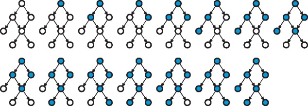
Consistent sub-graphs of an ontology $\mathcal{O}=(V,E)$ with $\left|V\right|=7$ vertices and $\left|E\right|=7$ edges, shown in the upper left-hand corner. There are 15 consistent sub-graphs of $\mathcal{O}$, as shown by coloring the appropriate groups of vertices in blue (the first graph represents the ontology and the empty sub-graph at the same time). Observe that the reversal of all edges in the graph would lead to a reversed graph with the same number of consistent sub-graphs (white vertices; Theorem 5.1)

We generally observe that the number of consistent sub-graphs is bounded from below by $2^{\ell }$, where $\ell$ is the total number of leaf vertices (those with no outgoing edges) and from above by $2^{\left|V\right|}$. The structure of the graph, however, determines the exact count and its proximity to either of the bounds. If the input graph is a chain of $\left|V\right|$ vertices ($\ell =1$), the total number of consistent sub-graphs equals $\left|V\right|+1$. On the other hand, if the original graph is a set of $\left|V\right|$ disconnected vertices ($\ell =\left|V\right|$), there are $2^{\left|V\right|}=2^{\ell }$ consistent sub-graphs. This analysis suggests that enumerating consistent sub-graphs has a straightforward intractable solution of listing all $2^{\left|V\right|}$ vertex-induced sub-graphs of the ontology and checking for the consistency of each such sub-graph.

We use $\mathtt{cdag}\left(\mathcal{O}\right)$ to denote the desired function that takes a DAG $\mathcal{O}$ as input and returns the number of consistent sub-graphs in that graph. We use $\mathtt{ctree}\left(\mathcal{T}\right)$ and $\mathtt{cforest}\left(\mathcal{F}\right)$ for the special cases where the input graph is a rooted tree $\mathcal{T}$ or a forest $\mathcal{F}$, respectively.

4.2 Counting sub-trees of trees

We first discuss a special case where the input graph is a rooted tree; that is, when each non-root vertex has a single parent. In this case, there exists a linear algorithm in the number of vertices; see Lemma 1 in Ruskey (1981). We provide this solution in Algorithm 1 with a minor modification resulting from the fact that our algorithm includes an empty tree in the total count. This algorithm naturally extends to collections of rooted trees. One can enumerate sub-trees for each tree and take the product as the total count. We refer to this extended algorithm as $\mathtt{cforest}$ (not shown).

Algorithm 1 .

Counting the number of consistent sub-graphs in rooted trees (Ruskey, 1981).

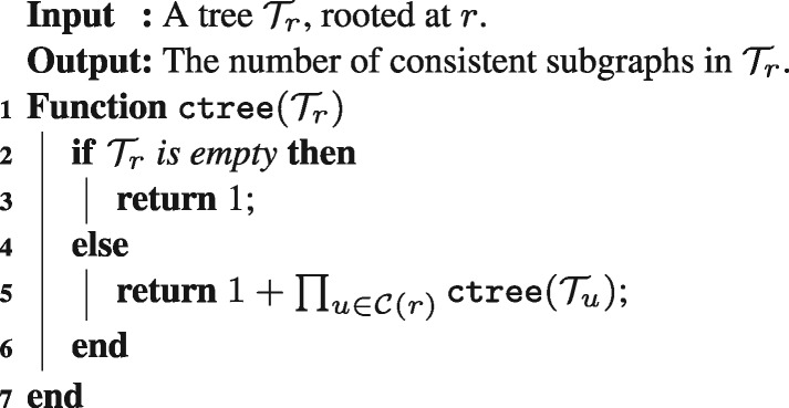
Algorithm 1 recursively traverses a tree in a pre-order manner. For any sub-tree rooted at vertex v, the number of consistent sub-trees that contain v equals the product of all sub-counts from its sub-trees rooted at each child. Additionally, we add 1 for the only consistent sub-tree that does not contain v; i.e. the empty tree. The recursion terminates at the empty tree whose count is one.

Algorithm 2 .

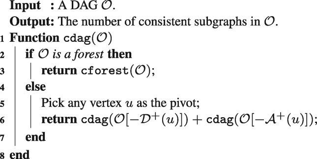
Counting the number of consistent sub-graphs in DAGs.

4.3 Counting consistent sub-graphs in DAGs

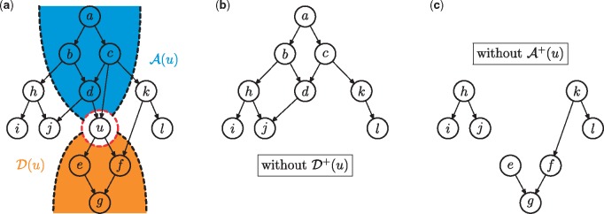
DAGs generalize trees in that they allow for multi-parent vertices. Such vertices, however, break Algorithm 1 because the recursive branches are no longer independent. Algorithm 2 circumvents this problem by recursively decomposing a graph into two strictly smaller sub-graphs according to a selected pivot vertex. We will show in the next section that the number of consistent sub-graphs in the two smaller graphs adds up to be the number for the original graph (Line 6, Algorithm 2). The algorithm continues recursive enumeration until the graph becomes a forest, in which case it calls $\mathtt{cforest}$. Figure 3 illustrates the process of graph decomposition with respect to the pivot vertex u. We note that any vertex can serve as pivot and will discuss the selection of pivots and how they impact the run time in Sections 5.3 and 6.1.

Fig. 3.

Illustration of graph decomposition. The enumeration problem of the original graph from panel (a) is split into two sub-problems based on the pivot vertex u; shown in panels (b) and (c). The count in (b) corresponds to the number of consistent sub-graphs in (a) that do not include u, while the count in (c) corresponds to the count of consistent sub-graphs in (a) that include u. In panel (a), the set of descendants of u is shaded in orange and the set of ancestors is shaded in blue. Notice that the re-occurrence of sub-graph h-i-j in both (b) and (c) offers the possibility of speed-ups by hashing

4.4 Correctness and complexity of the algorithm

We first observe that the size of the problem in the number of vertices is guaranteed to decrease during recursive calls, thus ensuring that the algorithm terminates after a finite number of iterations. Next, we justify the equation corresponding to the Line 6 in Algorithm 2,

$$\mathtt{cdag}\left(\mathcal{O}\right)=\mathtt{cdag}\left(\mathcal{O}[-{\mathcal{D}}^{+}(u\left)\right]\right)+\mathtt{cdag}\left(\mathcal{O}[-{\mathcal{A}}^{+}(u\left)\right]\right).$$ (1)

Lemma 4.1.

Let $\mathtt{cdag}\left(\mathcal{O}\right|\neg u)$ be the number of consistent sub-graphs in $\mathcal{O}$ that do not contain u. We have $\mathtt{cdag}\left(\mathcal{O}\right|\neg u)=\mathtt{cdag}(\mathcal{O}[-{\mathcal{D}}^{+}(u\left)\right])$.

Proof.

The equal cardinality of the two sets of consistent sub-graphs is demonstrated by showing that both sets are contained in each other. For any $S\subseteq V-{\mathcal{D}}^{+}\left(u\right)$ that induces a consistent sub-graph of $\mathcal{O}[-{\mathcal{D}}^{+}(u\left)\right]$, it also induces a unique consistent sub-graph in $\mathcal{O}$. Also, since none of them contains u, we have $\mathtt{cdag}\left(\mathcal{O}\right[-{\mathcal{D}}^{+}\left(u\right)\left]\right)\le \mathtt{cdag}\left(\mathcal{O}\right|\neg u)$. Conversely, for any consistent sub-graph induced by S such that $u\notin S$, we have $\forall v\in {\mathcal{D}}^{+}\left(u\right),v\notin S$ by the definition of consistency. Therefore, S also induces a consistent sub-graph in $\mathcal{O}[-{\mathcal{D}}^{+}(u\left)\right]$. That is, $\mathtt{cdag}\left(\mathcal{O}\right|\neg u)\le \mathtt{cdag}(\mathcal{O}[-{\mathcal{D}}^{+}(u\left)\right])$. □

Lemma 4.2.

Let $\mathtt{cdag}\left(\mathcal{O}\right|u)$ be the number of consistent sub-graphs in $\mathcal{O}$ that contain u. We have $\mathtt{cdag}\left(\mathcal{O}\right|u)=\mathtt{cdag}(\mathcal{O}[-{\mathcal{A}}^{+}(u\left)\right])$.

Proof.

As in Lemma 4.1, for any $S\subseteq V-{\mathcal{A}}^{+}\left(u\right)$ that induces a consistent sub-graph of $\mathcal{O}[-{\mathcal{A}}^{+}(u\left)\right],\hspace{0.17em}S\cup {\mathcal{A}}^{+}\left(u\right)$ also induces a unique consistent sub-graph (that contains u) in the original graph. That is, $\mathtt{cdag}\left(\mathcal{O}\right[-{\mathcal{A}}^{+}\left(u\right)\left]\right)\le \mathtt{cdag}\left(\mathcal{O}\right|u)$. Also, for any consistent sub-graph induced by S and $u\in S$, we have ${\mathcal{A}}^{+}\left(u\right)\subseteq S$ by the definition of consistency. Note that the uniqueness of S implies the uniqueness of $S-{\mathcal{A}}^{+}\left(u\right)$. We can see that the sub-graph induced by $S-{\mathcal{A}}^{+}\left(u\right)$ in $\mathcal{O}[-{\mathcal{A}}^{+}(u\left)\right]$ is consistent. Given $\forall w\in S-{\mathcal{A}}^{+}\left(u\right)$, and (v, w) being an edge in $\mathcal{O}[-{\mathcal{A}}^{+}(u\left)\right]$, we must have $v\in S-{\mathcal{A}}^{+}\left(u\right)$ as well, due to the consistency of $\mathcal{O}\left[S\right]$ with respect to the original graph. That is, $\mathtt{cdag}\left(\mathcal{O}\right|u)\le \mathtt{cdag}(\mathcal{O}[-{\mathcal{A}}^{+}(u\left)\right])$. □

Theorem 4.1.

Given an ontology $\mathcal{O}=(V,E)$ and any $u\in V$, the number of consistent sub-graphs in $\mathcal{O}$ equals the sum of the numbers of consistent sub-graphs in $\mathcal{O}[-{\mathcal{D}}^{+}(u\left)\right]$ and $\mathcal{O}[-{\mathcal{A}}^{+}(u\left)\right]$.

Proof.

Equation (1) holds by combining Lemmas 4.1 and 4.2. □

To analyze complexity of the algorithm, let n be the number of vertices in the graph and m be the number of multi-parent vertices. Assuming a multi-parent vertex is always selected as pivot, we can express the run time complexity T(n) via the following recurrence

$$T\left(n\right)\le T(n-1)+T(n-3)+f\left(n\right),$$

where f(n) incorporates the time to select the pivot, split the graph and add two large integers. Let us further assume that the larger of the two graphs after decomposition contains $n-n/k$ elements, where $2\le k\le n$. It is now straightforward to show that $T\left(n\right)=O\left(f\right(n\left)2^{\min (m,s(k\left)\right)}\right)$, where $s\left(k\right)=O\left(n\right)$ if $k=O\left(n\right)$ and $s\left(k\right)=O(\text{log}\hspace{0.17em}n)$ if $k=O\left(1\right)$.

We can now see that the algorithm is exponential in the worst case; however, it reduces to a polynomial algorithm when $m=O(\text{log}\hspace{0.17em}n)$ or when $k=O\left(1\right)$. Assuming linear time to conduct graph decomposition and a constant time for addition/multiplication, we obtain $T\left(n\right)=O\left(n^2\right)$.

5 Accelerations

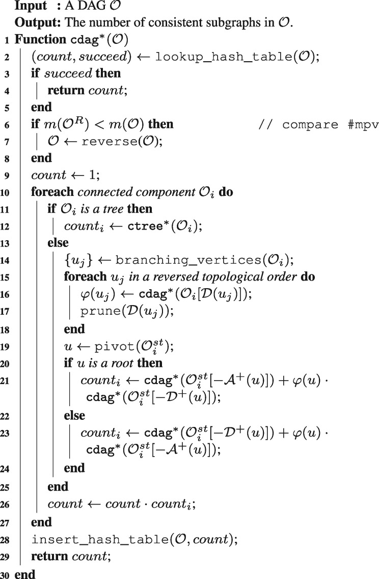
The run-time of the algorithm heavily depends on the structure of the ontology and the selection of pivots. Here, we discuss several practical considerations aimed at accelerating Algorithm 2. Once we conclude this discussion, the full method will be presented in Algorithm 3 (Section 6).

5.1 Pruning branching components

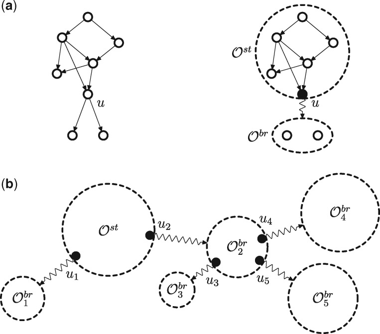
It is easy to observe that when the ontology consists of multiple connected components, these components can be independently and, if needed, simultaneously processed. We take this reasoning a step further to consider a special scenario of nearly disconnected graphs where (i) the two components are connected via a single vertex and (ii) all vertices in one component are descendants of this vertex.

Definition 5.1.

Given a graph $\mathcal{O}=(V,E)$ and $u\in V,\hspace{0.17em}\mathcal{O}\left[\mathcal{D}\right(u\left)\right]$ is called a branching component if$\forall v\in V-{\mathcal{D}}^{+}\left(u\right)$and$\forall w\in \mathcal{D}\left(u\right),(v,w)\notin E$. Vertex u is called a branching vertex.

Figure 4a gives an example in which u is a branching vertex, since the removal of u disconnects $\mathcal{D}\left(u\right)$ (i.e. the branching component, ${\mathcal{O}}^{\text{br}}$) from the rest of the graph. We refer to the remaining part of the graph as the stem component, ${\mathcal{O}}^{\text{st}}$. More generally, Figure 4b shows a graph with a component-wise tree structure, where branching vertices serve as hinges of branching component to their corresponding stems. We will use $({\mathcal{O}}^{\text{st}},{\mathcal{O}}^{\text{br}},u)$ to denote the desired structure.

Fig. 4.

Illustration of branching components. Panel (a) shows a branching vertex u that separates the graph into a stem component ${\mathcal{O}}^{\text{st}}$ and a branching component ${\mathcal{O}}^{\text{br}}$. The collection of edges from u to ${\mathcal{O}}^{\text{br}}$ is replaced by a zigzag arrow. Panel (b) shows a component-wise tree structure

Given $({\mathcal{O}}^{\text{st}},{\mathcal{O}}^{\text{br}},u)$, we demonstrate that $\mathtt{cdag}\left(\mathcal{O}\right)$ can be decoupled into two sequential sub-problems: (i) $\mathtt{cdag}({\mathcal{O}}^{\text{br}})$ and (ii) $\mathtt{cdag}\left({\mathcal{O}}^{\text{st}}\right)$. We use $\phi \left(u\right)$ for the sub-total of consistent sub-graphs in the branching component ${\mathcal{O}}^{\text{br}}$. We also notice that the entire branching component can be pruned once $\phi \left(u\right)$ is computed, making u a leaf vertex in ${\mathcal{O}}^{\text{st}}$. Therefore, we modify the algorithm so as to allow a sub-total count $\phi \left(u\right)$ for every vertex as if a branching component has been pruned from u. Notice that $\phi \left(u\right)=1$ for all intermediate vertices and original leaves.

With the introduction of $\phi \left(u\right)$, the recursive equation in Algorithm 1 becomes

$$\mathtt{ctree}\left({\mathcal{T}}_r\right)=\phi \left(r\right)+\prod _{u\in \mathcal{C}\left(r\right)}\mathtt{ctree}\left({\mathcal{T}}_u\right).$$ (2)

Similarly, Equation (1); i.e. Line 6 in Algorithm 2, must be modified to

$$\mathtt{cdag}\left({\mathcal{O}}^{\text{st}}\right)=\mathtt{cdag}\left({\mathcal{O}}^{\text{st}}[-{\mathcal{D}}^{+}(u\left)\right]\right)+\phi \left(u\right)·\mathtt{cdag}\left({\mathcal{O}}^{\text{st}}[-{\mathcal{A}}^{+}(u\left)\right]\right),$$ (3)

where $\phi \left(u\right)$ accounts for the fact that for any consistent sub-graph S_i in the pruned ${\mathcal{O}}^{\text{br}}$ and any consistent sub-graph S_j in ${\mathcal{O}}^{\text{st}}[-{\mathcal{A}}^{+}(u\left)\right],\hspace{0.17em}\mathcal{O}[S_i\cup S_j\cup {\mathcal{A}}^{+}(u\left)\right]$ is a distinct consistent sub-graph in $\mathcal{O}$. The approach naturally extends to multiple (hierachical) branching components such that we compute the sub-total of consistent sub-graphs within each component and agglomerate them in a reversed topological order.

The pruning operation is preferred before each instance of decomposition for two main reasons: (i) it divides the problem into smaller non-overlapping sub-problems, while a direct decomposition usually results in substantial overlapping sub-problems; (ii) although a full parallelization over components is restricted since stem components have to be computed only after all of their branching components are finished, the unordered components can be computed simultaneously. For example, as in Figure 4b, ${\mathcal{O}}_1^{\text{br}},\hspace{0.17em}{\mathcal{O}}_3^{\text{br}},\hspace{0.17em}{\mathcal{O}}_4^{\text{br}}$ and ${\mathcal{O}}_5^{\text{br}}$ can be computed in parallel.

5.2 Reverse graphs

Let ${\mathcal{O}}^R=(V,E^R)$ be the reverse graph of $\mathcal{O}$, where $E^R=\left\{\right(u,v\left)\right|(v,u)\in E\}$. We show that the number of consistent sub-graphs in $\mathcal{O}$ equals that in ${\mathcal{O}}^R$.

Lemma 5.1.

If $\mathcal{O}\left[S\right]$ is a consistent sub-graph of $\mathcal{O},\hspace{0.17em}{\mathcal{O}}^R[-S]$ is a consistent sub-graph of ${\mathcal{O}}^R$.

Proof.

We prove this Lemma by contradiction. For $\forall u\in V-S$ and $\forall v\in {\mathcal{A}}^R\left(u\right)$ [We use ${\mathcal{A}}^R\left(u\right)$ and ${\mathcal{D}}^R\left(u\right)$ for ancestors and descendants of u in ${\mathcal{O}}^R$; ${\mathcal{A}}^R\left(u\right)=\mathcal{D}\left(u\right)$ and ${\mathcal{D}}^R\left(u\right)=\mathcal{A}\left(u\right)$], if $v\notin V-S$, then $u\in \mathcal{A}\left(v\right)\subseteq S$ due to the consistency of $\mathcal{O}\left[S\right]$. This contradicts $u\in V-S$. Therefore, the assumption $v\notin V-S$ is false and we have $\forall u\in V-S,\hspace{0.17em}\forall v\in {\mathcal{A}}^R\left(u\right)\subseteq V-S$. That is, ${\mathcal{O}}^R[-S]$ is consistent.

This Lemma demonstrates that all complementary white vertices in Figure 2 form consistent sub-graphs in the reverse graph.

Theorem 5.1.

Given an ontology $\mathcal{O},\hspace{0.17em}\mathtt{cdag}\left(\mathcal{O}\right)=\mathtt{cdag}\left({\mathcal{O}}^R\right)$.

Proof.

Given Lemma 5.1, we see that the mapping $f\left(\mathcal{O}\right[S\left]\right)={\mathcal{O}}^R[-S]$ is a bijection between the two sets of consistent sub-graphs. Therefore, the two sets are of equal cardinality.

Theorem 5.1

permits graph reversal at any point during the algorithm depending on which of the graphs is more likely to terminate first. For example, we can always choose the one with fewer multi-parent vertices so as to greedily reduce the upper bound of recursive calls. It is worth noting that all the leaves become roots in the reverse graph. Therefore, in the final algorithm that incorporates both pruning and reversing modules, we generalize the algorithm to allow for $\phi >1$ on roots (branching vertices in the reverse sense) in order to ensure compatibility.

Having $\phi \left(r\right)>1$ on a root indicates that all the ancestors of r have been pruned out. For trees (after pruning), we have $\mathcal{O}[-{\mathcal{D}}^{+}(r\left)\right]=\mathcal{O}\left[\mathcal{A}\right(r\left)\right]$. With Lemma 4.1 and Theorem 5.1, we have

$$\mathtt{cdag}\left(\mathcal{O}\right|\neg r)=\mathtt{cdag}(\mathcal{O}[-{\mathcal{D}}^{+}(r\left)\right])=\mathtt{cdag}(\mathcal{O}\left[\mathcal{A}\right(r\left)\right])$$

$$=\mathtt{cdag}\left({\mathcal{O}}^R\right[{\mathcal{D}}^R\left(r\right)\left]\right)=\phi \left(r\right).$$

On the other hand, for any consistent sub-graph S containing r, $S-{\mathcal{A}}^{+}\left(r\right)$ induces a consistent sub-graph in $\mathcal{O}\left[\mathcal{D}\right(r\left)\right]$ and vice versa; thus,

$$\mathtt{cdag}\left(\mathcal{O}\right|r)=\prod _{u\in \mathcal{C}\left(r\right)}\mathtt{ctree}({\mathcal{T}}_u).$$

Hence, these two sub-totals sum to be the total count and Equation (2) remains unchanged. However, if a root r with $\phi \left(r\right)>1$ is selected to be the pivot, we have the following equation according to Theorem 5.1 and Equation (3),

$$\mathtt{cdag}\left(\mathcal{O}\right)=\mathtt{cdag}\left({\mathcal{O}}^R\right)$$

$$=\mathtt{cdag}\left({\mathcal{O}}^R\right[-{\mathcal{D}}^{R+}\left(r\right)\left]\right)+\phi \left(r\right)·\mathtt{cdag}\left({\mathcal{O}}^R\right[-{\mathcal{A}}^{R+}\left(r\right)\left]\right)$$

$$=\mathtt{cdag}\left(\mathcal{O}\right[-{\mathcal{A}}^{+}\left(r\right)\left]\right)+\phi \left(r\right)·\mathtt{cdag}\left(\mathcal{O}\right[-{\mathcal{D}}^{+}\left(r\right)\left]\right),$$

whereas Equation (3) remains unchanged for non-root vertices.

5.3 Pivot selection

As alluded to before, the selection of vertices used for partitioning has the potential to significantly change the computation time. It is therefore reasonable to devise a strategy for pivot selection. Besides a random selection of multi-parent vertices (mpv’s), which aims at directly converting DAGs into trees one step at a time, we also consider three other pivot heuristics. The first strategy is to pick a vertex with the maximum degree, with random selection in case of ties, because decomposing the graph according to such vertices may increase the chance of having either disconnected components or branching components. The second strategy selects the pivot so as to minimize $e-n+r$ over the two sub-problems, where e, n and r are the number of edges, vertices and roots in the two components. We refer to this quantity as ‘bound’ since it is an upper bound of the number of mpv’s in the graph (see Supplementary Material for the proof). Note that it is closely related to the cyclomatic number of the graph. Finally, the third strategy simulates a unit network flow for all vertices running in the direction from leaves to the roots and selects the ‘bottleneck’ vertex; i.e. the one that maximizes the ratio of the flow in the vertex and the number of its descendants (see Supplementary Material for this pivot selection algorithm). These strategies will be empirically compared in Section 6.

5.4 Hashing

It can occur during the recursive procedure that certain sub-graphs require repeated enumeration. In Figure 3, for example, the sub-graph h-i-j is present in both sub-problems shown in Figure 3b–c. Computing the count for this sub-graph would emerge in the Figure 3b sub-problem if the ensuing decomposition were based on vertex d, although it would not emerge if the partitioning were based on vertex j. Interestingly, the sub-graph k-l would be counted twice in the Figure 3b sub-problem; i.e. when both ${\mathcal{A}}^{+}\left(d\right)$ and ${\mathcal{D}}^{+}\left(d\right)$ are removed, and it would then appear one more time in the Figure 3c sub-problem.

To avoid repeated enumeration, whenever a solution to a sub-problem is obtained, the count for this sub-problem is stored. Then, during the recursive calls, we first check if the result is already available before further calculation. To hash a result, we use the sorted IDs of all vertices in the sub-graph as a key. Obviously, this key is unique because it corresponds to a vertex-induced sub-graph of $\mathcal{O}$. For the pruned sub-graph, we store the key of the sub-graph along with the branching vertex. Whenever the ID of the branching vertex is used to generate a key, the stored key of the corresponding sub-graph is appended to the vertex’s ID with parentheses around it.

Algorithm 3 .

The advanced version of Algorithm 2 with optimization modules.

6 Experiments and results

We empirically evaluate the enumeration procedure from Algorithm 3 and various practical speedups using randomly generated graphs. We then apply this algorithm to four biomedical ontologies to gain insight into the sizes of their concept annotation spaces.

6.1 Run-time evaluation

We generated two sets of graphs to investigate the efficacy of our algorithm. Each set contained 1000 graphs with either 25 or 100 vertices. To construct each graph the vertices were added sequentially, with the proposed in-degree in-deg(v) of the k-th vertex v generated according to a Poisson distribution with parameter λ. This vertex then became a child of $\min$(in-deg(v), k – 1) previously generated vertices that were themselves selected uniformly randomly. The parameter λ was selected according to the $\Gamma (2.0,1.0)$ prior for each new graph and kept constant until the graph was completed.

With these two sets of simulated graphs, we ran our algorithm with different modules and pivot selection strategies. In particular, we evaluate pivot selection based on (i) random selection of vertices, (ii) random selection of multi-parent vertices, (iii) the degree criterion, (iv) the bound criterion and (v) the bottleneck criterion. For each pivoting strategy, we subsequently add the pruning component, then hashing and finally graph reversal. The criterion for graph reversal was the number of multi-parent vertices; i.e. a graph will be reversed at any point during the recursive process if the reversed graph contains fewer multi-parent vertices.

We report the average wall-time and average number of recursive calls over the two sets of 1000 graphs ($\left|V\right|=25$ in Table 1; $\left|V\right|=100$ in Table 2). For the smaller graphs, we also ran a brute-force algorithm that was further convenient to empirically evaluate the correctness of our algorithm. The brute-force algorithm generates each of the $2^{\left|V\right|}$ subsets of nodes and then performs a consistency check. We see that simpler schemes perform better on small graphs where the number of recursive calls per graph has not exceeded a few hundreds. On the other hand, the advanced techniques show tangible benefits on the larger graphs reducing the number of recursive calls and total computation time by orders of magnitude. It is possible to envision other variations that could result in further speedups; e.g. selecting multi-parent pivots with the highest degree. These refinements, however, were beyond the scope of this paper.

Table 1.

Experiments with simulated graphs with $\left|V\right|=25$ vertices

Brute-force	Module	Random	Random mpv	Min. bound	Max. degree	Bottleneck
571 ms		22.5 ms (313)	5.3 ms (39)	25.7 ms (23)	1.2 ms (28)	18.2 ms (47)
		21.1 ms (97)	14.3 ms (44)	26.4 ms (25)	10.2 ms (28)	25.3 ms (44)
		19.6 ms (71)	14.4 ms (39)	26.3 ms (23)	10.2 ms (26)	24.9 ms (34)
		19.2 ms (67)	7.5 ms (28)	25.5 ms (23)	7.5 ms (23)	23.9 ms (31)

Notes: Each field in the table summarizes the per-graph wall-time over a set of 1000 graphs as well as the per-graph number of recursive calls, except for the brute-force method. The columns represent pivot selection strategies: (i) random, (ii) random multi-parent vertex (mpv), (iii) minimum bound, (iv) maximum degree and (v) bottleneck. The rows represent successive additions of practical modules for speedups: () basic approach from Algorithm 2, () pruning, () pruning and hashing, () pruning, hashing and graph reversal.

Table 2.

Experiments with simulated graphs with $\left|V\right|=100$ vertices, with rows and columns identical to those in Table 1

Module	Random	Random mpv	Min. bound	Max. degree	Bottleneck
	*3102 s (119 745 876)	5.21 s (52 954)	114 s (25 416)	9.93 s (101 342)	122 s (526 925)
	323 s (2 337 554)	8.98 s (33 271)	3.93 s (2802)	1.10 s (3066)	4.28 s (12 597)
	157 s (457 075)	7.35 s (14 913)	3.67 s (1111)	0.92 s (1107)	3.08 s (2052)
	165 s (508 521)	4.68 s (9721)	3.22 s (1103)	0.84 s (1079)	2.79 s (2133)

Notes: The entry with an asterisk indicates that a sample of three graphs was considered (instead of a full set of 1000) due to the long run-time. The brute-force algorithm was not considered as it was not feasible to compute the count for even a single graph.

6.2 Consistent sub-graphs in biomedical ontologies

We use 02/2017 versions of GO and Human Phenotype Ontology (HPO) as the target ontologies and compute the number of consistent sub-graphs in each of them. The algorithm is applied to each of the three domains of GO (Ashburner et al., 2000): (i) molecular function ontology (MFO; 10 789 terms) (ii) biological process ontology (BPO; 29 575 terms) and (iii) cellular component ontology (CCO; 4085 terms). Together with HPO (12 167 terms), these four ontologies are widely used in annotating functional terms of gene products (Jiang et al., 2016; Radivojac et al., 2013). We further define the annotation level for each term in the ontology to be the length of the longest path to the root. Starting from the root term, we add more specific terms level-by-level to understand how the potential annotation space grows with increased granularity of functional concepts.

In addition to level-wise full ontologies, we also investigate the ‘used’ ontologies in which each term was retained only if at least one protein in the UniProt-GOA (Huntley et al., 2015) and HPO (Robinson and Mundlos, 2010) databases has been confidently assigned that term (confident annotations include all experimental evidence codes as well as ‘traceable author statement’ and ‘inferred by curators’). Protein function annotations were extracted from the 02/13/2017 release of the UniProt-GOA database, which contains 64 362 proteins with confident MFO annotations, 84 413 proteins with BPO annotations and 79 630 proteins with CCO annotations. HPO annotations were extracted from the 02/24/2017 release of the HPO database where 6411 genes with confident annotations were extracted.

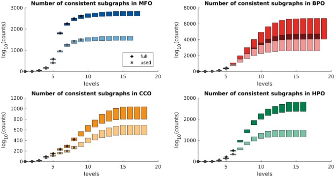
Figure 5 shows the completed counts for both full and used level-wise ontologies. For each ontology, we additionally compute the lower bound (generally the larger of $2^{\ell }$ and $2^r$, where $\ell$ is the number of leaves and r is the number of roots) and estimate the upper bound (we convert a graph into a forest by keeping only one randomly selected incoming edge for each multi-parent vertex and then call $\mathtt{cforest}$). The counts of consistent sub-graphs grow rapidly as more specific terms are included and later plateau.

Fig. 5.

Number of consistent sub-graphs in level-wise GO and HPO (see Supplementary Table S1 for exact counts). In each panel, black + symbols mark the exact counts for ‘full’ sub-graphs and grey × symbols mark the exact counts for ‘used’ sub-graphs. Colored boxes indicate the estimated upper/lower bounds of the actual counts, with darker boxes corresponding to ‘full’ ontologies and lighted boxes corresponding to ‘used’ ontologies at a particular level. The exact integer counts are available upon request

Although we were not surprised by the astronomical sizes of concept annotation spaces; e.g. MFO terms up to the level of 9 create $2.036\times {10}^{2616}$ consistent sub-graphs, it was rewarding to provide exact counts whenever feasible as well as to observe an increasing difference between lower and upper bounds (in the 100 s to 1000 s of orders of magnitude) with the level of the ontology. We also find it interesting that a large number of ontological terms have never been used to annotate a gene or a protein; i.e. 31% of terms in GO and 44% of terms in HPO (Supplementary Material). Finally, using the number of recursive calls of our algorithm (Supplementary Material) as a measure of graph complexity, we observe an inverse relationship between the graph complexity and the accuracy of the top function prediction algorithms in the Critical Assessment of Functional Annotation experiments (Jiang et al., 2016; Radivojac et al., 2013). Although some complexity of the available ontologies can be attributed to the level of biological abstraction they are intended to describe (e.g. Biological Process), it is reasonable to consider that the structure of the ontology itself is a contributing factor to a lower prediction accuracy. As an example, we note that both Molecular Function and Cellular Component annotations correspond to relatively straightforward biological concepts, yet MFO is significantly simpler than CCO; e.g. it contains a smaller fraction of multi-parent vertices, it has lower graph edge density and, correspondingly, it had fewer recursive calls by our algorithm. In agreement with this consideration, the accuracy of concept prediction in MFO exceeds the accuracy currently observed in CCO, even when data biases are accounted for (Jiang et al., 2016).

6.3 Entropy of concept annotation spaces

The ability to enumerate sub-graphs in relatively large ontologies presents an opportunity to contrast the space of actual ontological annotations in biological databases with the space of possible ontological annotations. To investigate this, we first computed the entropy of actual annotations at different levels in the ontology,

$$H\left({\mathcal{O}}_{lvl}\right)=-\sum _{i}P\left({\mathcal{O}}_{lvl}\right[S_i\left]\right)\hspace{0.17em}{\text{log}}_{2}P\left({\mathcal{O}}_{lvl}\right[S_i\left]\right),$$

where ${\mathcal{O}}_{lvl}$ is the truncated ontology as in Section 6.2, ${\mathcal{O}}_{lvl}\left[S_i\right]$ corresponds to a distinct consistent sub-graph annotation observed at that level and $P\left({\mathcal{O}}_{lvl}\right[S_i\left]\right)$ is the probability that a protein is assigned annotation ${\mathcal{O}}_{lvl}\left[S_i\right]$. We first enumerated all observed sub-graphs from the UniProt-GOA or HPO database truncated to a particular level, calculated their relative frequencies, and then plugged these relative frequencies into the entropy formula above. On the other hand, the maximum entropy was computed as $\hspace{0.17em}{\text{log}}_2\mathtt{cdag}\left({\mathcal{O}}_{lvl}\right)$ by assuming equal probability for every possible consistent sub-graph.

Figure 6 shows the ratio between the two quantities for levels greater than 1, suggesting that the world of protein functions, despite great diversity, has low entropy relative to the possible maximum. Although the currently observed functional annotations are incomplete, noisy and biased (Jiang et al., 2014; Schnoes et al., 2009, 2013), this suggests considerable departure from the uniform distribution.

Fig. 6.

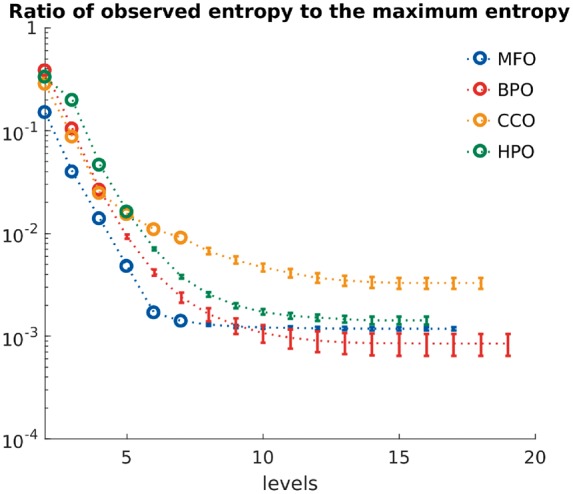
Ratio of entropies in the four ontologies. Colored circles show the ratio of the observed entropy to the maximum entropy for each level in the evaluated ontologies. Dotted lines correspond to the estimated ratios as the average of the two ratios calculated by lower/upper bound of the counts. The error bars suggest a possible placement for the actual ratio

7 Related work

There exists a body of literature in enumerative combinatorics related to our work. One of the most relevant problems is the enumeration of DAGs with n distinct (labeled) nodes (Robinson, 1971). The resulting count reflects the size of the structure space of Bayesian networks with n random variables and, surprisingly, also corresponds to the number of matrices in ${\left\{0,1\right\}}^{n\times n}$ with all eigenvalues real and positive (McKay et al., 2004). The number of labeled DAGs with n nodes does not have a closed-form solution and is instead available as the A003024 sequence in the On-Line Encyclopedia of Integer Sequences (OEIS); https://oeis.org/A003024. The construction was originally proposed by Robinson (1971) and was further investigated by others (Gessel, 1996; Rodionov, 1992; Stanley, 1973).

Previous findings on rooted labeled trees include both the enumeration of possible number of trees and also the enumeration of sub-trees for a given tree. There are $n^{n-1}$ labeled rooted trees with n nodes (Gross and Yellen, 2004) that provide the integer sequence A000169 in OEIS; https://oeis.org/A000169. The expansion to forests gives ${(n+1)}^{n-1}$ using Cayley’s formula (Cayley, 1889), as a single root can be added to connect a forest of unrooted labeled trees into a rooted labeled tree. The recurrence for the number of sub-trees of a given tree was proposed by Ruskey (1981); see Algorithm 1. The generalization to weighted sub-trees was given by Yan and Yeh (2006). Both algorithms are linear in n assuming constant time addition and multiplication.

The research in ontology quality assurance is another related problem. These efforts typically include the analysis of irregularities and redundancy in concept descriptors and graph structure (Bodenreider, 2003; Verspoor et al., 2009; Xing et al., 2016). Our work, primarily the software we developed, contributes to this area by facilitating the analysis of the annotation space.

8 Conclusions

This work presents a practical algorithm for enumerating consistent sub-graphs of DAGs. We build upon the work of Ruskey (1981) and Yan and Yeh (2006), who solved the sub-structure enumeration problems in trees, by providing a non-trivial extension to DAGs. However, we also believe that our algorithm has practical utility for the studies of ontological annotation spaces that have recently gained popularity in structured-output learning in computational biology and other fields (Grosshans et al., 2014; Joachims et al., 2009; Movshovitz-Attias et al., 2015; Radivojac et al., 2013; Sokolov and Ben-Hur, 2010). Another related problem is workflow enumeration that may have implications on code analysis and debugging in distributed computing environments (Sadiq and Orlowska, 2000; Zaharia et al., 2010).

The observed outcomes on biomedical ontologies raise important questions regarding the predictability of ontological annotations because most modern algorithms are asked to provide accurate deep annotations to have practical utility. However, annotation spaces become exceedingly large almost instantaneously with the depth of the ontology, which presents an immense computational and statistical challenge for any prediction algorithm. We therefore believe that the balance between ontology size/complexity and term granularity should become an important topic for future discussions among biocurators and function prediction researchers.

Funding

This work has been supported by the National Science Foundation grant DBI-1458477 and the Indiana University Precision Health Initiative. The authors thank Kymberleigh Pagel for helpful comments.

Conflict of Interest: none declared.

References

- Ashburner M. et al. (2000) Gene ontology: tool for the unification of biology. The Gene Ontology Consortium. Nat. Genet., 25, 25–29. [DOI] [PMC free article] [PubMed] [Google Scholar]
- Bodenreider O. (2003) Strength in numbers: exploring redundancy in hierarchical relations across biomedical terminologies. AMIA Annu. Symp. Proc., 101–105. [PMC free article] [PubMed] [Google Scholar]
- Cayley A. (1889) A theorem on trees. Quart. J. Math., 23, 376–378. [Google Scholar]
- Clark W.T., Radivojac P. (2013) Information-theoretic evaluation of predicted ontological annotations. Bioinformatics, 29, i53–i61. [DOI] [PMC free article] [PubMed] [Google Scholar]
- Friedberg I., Radivojac P. (2017) Community-wide evaluation of computational function prediction. Methods Mol. Biol., 1446, 133–146. [DOI] [PubMed] [Google Scholar]
- Gessel I.M. (1996) Counting acyclic digraphs by sources and sinks. Discrete Math., 160, 253–258. [Google Scholar]
- Gross J.L., Yellen J. (2004) Handbook of Graph Theory. CRC Press, Boca Raton, Florida, USA. [Google Scholar]
- Grosshans M. et al. (2014) Joint prediction of topics in a URL hierarchy. In: Proceedings of the Joint European Conference on Machine Learning and Knowledge Discovery in Databases, ECML/PKDD 2014. Springer, Nancy, France, pp. 514–529.
- Huntley R.P. et al. (2015) The GOA database: gene Ontology annotation updates for 2015. Nucleic Acids Res., 43, D1057–D1063. [DOI] [PMC free article] [PubMed] [Google Scholar]
- Jiang Y. et al. (2014) The impact of incomplete knowledge on the evaluation of protein function prediction: a structured-output learning perspective. Bioinformatics, 30, i609–i616. [DOI] [PMC free article] [PubMed] [Google Scholar]
- Jiang Y. et al. (2016) An expanded evaluation of protein function prediction methods shows an improvement in accuracy. Genome Biol., 17, 184.. [DOI] [PMC free article] [PubMed] [Google Scholar]
- Joachims T. et al. (2009) Cutting-plane training of structural SVMs. Mach. Learn., 77, 27–59. [Google Scholar]
- Joslyn C.A. et al. (2004) The gene ontology categorizer. Bioinformatics, 20, i169–i177. [DOI] [PubMed] [Google Scholar]
- Lord P.W. et al. (2003) Investigating semantic similarity measures across the Gene Ontology: the relationship between sequence and annotation. Bioinformatics, 19, 1275–1283. [DOI] [PubMed] [Google Scholar]
- McKay B.D. et al. (2004) Acyclic digraphs and eigenvalues of (0, 1)-matrices. J. Integer Seq., 7, 04.3.3. [Google Scholar]
- Moreau Y., Tranchevent L.C. (2012) Computational tools for prioritizing candidate genes: boosting disease gene discovery. Nat. Rev. Genet., 13, 523–536. [DOI] [PubMed] [Google Scholar]
- Movshovitz-Attias Y. et al. (2015) Ontological supervision for fine grained classification of street view storefronts. In: Proceedings of the IEEE Conference on Computer Vision and Pattern Recognition, CVPR 2015. IEEE, Boston, MA, USA, pp. 1693–1702.
- Pesquita C. (2017) Semantic similarity in the Gene Ontology. Methods Mol. Biol., 1446, 161–173. [DOI] [PubMed] [Google Scholar]
- Poux S., Gaudet P. (2017) Best practices in manual annotation with the Gene Ontology. Methods Mol. Biol., 1446, 41–54. [DOI] [PubMed] [Google Scholar]
- Radivojac P. et al. (2013) A large-scale evaluation of computational protein function prediction. Nat. Methods, 10, 221–227. [DOI] [PMC free article] [PubMed] [Google Scholar]
- Robinson P.N., Bauer S. (2011) Introduction to Bio-Ontologies. CRC Press, Boca Raton, Florida, USA. [Google Scholar]
- Robinson P.N., Mundlos S. (2010) The human phenotype ontology. Clin. Genet., 77, 525–534. [DOI] [PubMed] [Google Scholar]
- Robinson R.W. (1971) Counting labeled acyclic digraphs. In: Proceedings of the 3rd Ann Arbor Conference on Graph Theory. Academic Press, Ann Arbor, MI, USA, pp. 239–273.
- Rodionov V.I. (1992) On the number of labeled acyclic digraphs. Discrete Math., 105, 319–321. [Google Scholar]
- Ruskey F. (1981) Listing and counting subtrees of a tree. SIAM J. Comput., 10, 141–151. [Google Scholar]
- Sadiq W., Orlowska M.E. (2000) Analyzing process models using graph reduction techniques. Inf. Syst. J., 25, 117–134. [Google Scholar]
- Schnoes A.M. et al. (2009) Annotation error in public databases: misannotation of molecular function in enzyme superfamilies. PLoS Comput. Biol., 5, e1000605.. [DOI] [PMC free article] [PubMed] [Google Scholar]
- Schnoes A.M. et al. (2013) Biases in the experimental annotations of protein function and their effect on our understanding of protein function space. PLoS Comput. Biol., 9, e1003063.. [DOI] [PMC free article] [PubMed] [Google Scholar]
- Sokolov A., Ben-Hur A. (2010) Hierarchical classification of gene ontology terms using the GOstruct method. J. Bioinform. Comput. Biol., 8, 357–376. [DOI] [PubMed] [Google Scholar]
- Stanley R.P. (1973) Acyclic orientations of graphs. Discrete Math., 5, 171–178. [Google Scholar]
- Verspoor K. et al. (2006) A categorization approach to automated ontological function annotation. Protein Sci., 15, 1544–1549. [DOI] [PMC free article] [PubMed] [Google Scholar]
- Verspoor K. et al. (2009) Ontology quality assurance through analysis of term transformations. Bioinformatics, 25, i77–i84. [DOI] [PMC free article] [PubMed] [Google Scholar]
- Vihinen M. (2014) Variation Ontology for annotation of variation effects and mechanisms. Genome Res., 24, 356–364. [DOI] [PMC free article] [PubMed] [Google Scholar]
- Xing G. et al. (2016) FEDRR: fast, exhaustive detection of redundant hierarchical relations for quality improvement of large biomedical ontologies. BioData Min., 9, 31.. [DOI] [PMC free article] [PubMed] [Google Scholar]
- Yan W., Yeh Y.N. (2006) Enumeration of subtrees of trees. Theor. Comput. Sci., 369, 256–268. [Google Scholar]
- Zaharia M. et al. (2010) Spark: cluster computing with working sets. In: Proceedings of the 2nd USENIX Conference on Hot Topics in Cloud Computing. HotCloud 2010. Berkeley, CA, USA, p. 10.
Associated Data
This section collects any data citations, data availability statements, or supplementary materials included in this article.