Brain Tissue Segmentation Based on Diffusion MRI Using ℓ₀ Sparse-Group Representation Classification

Abstract

We present a method for automated brain tissue segmentation based on diffusion MRI. This provides information that is complementary to structural MRI and facilitates fusion of information between the two imaging modalities. Unlike existing segmentation approaches that are based on diffusion tensor imaging (DTI), our method explicitly models the coexistence of various diffusion compartments within each voxel owing to different tissue types and different fiber orientations. This results in improved segmentation in regions with white matter crossings and in regions susceptible to partial volume effects. For each voxel, we tease apart possible signal contributions from white matter (WM), gray matter (GM), and cerebrospinal fluid (CSF) with the help of diffusion exemplars, which are representative signals associated with each tissue type. Each voxel is then classified by determining which of the WM, GM, or CSF diffusion exemplar groups explains the signal better with the least fitting residual. Fitting is performed using ℓ₀ sparse-group approximation, circumventing various reported limitations of ℓ₁ fitting. In addition, to promote spatial regularity, we introduce a smoothing technique that is based on ℓ₀ gradient minimization, which can be viewed as the ℓ₀ version of total variation (TV) smoothing. Compared with the latter, our smoothing technique, which also incorporates multi-channel WM, GM, and CSF concurrent smoothing, yields marked improvement in preserving boundary contrast and consequently reduces segmentation bias caused by smoothing at tissue boundaries. The results produced by our method are in good agreement with segmentation based on T₁-weighted images.

1 Introduction

Brain tissue segmentation is most commonly performed using T₁-weighted images, which are typically rich with anatomical details thanks to their higher spatial resolution (1 × 1 × 1 mm³). However, the recent availability of high spatial resolution (1.25 × 1.25 × 1.25 mm³) diffusion MRI data from the Human Connectome Project¹ begs the following questions: 1) Can tissue segmentation be performed equally well solely based on diffusion data, therefore making it possible to avoid the technical difficulties involved in transferring segmentation information from T₁-weighted images, such as geometric distortion and cross-modality registration? 2) Can diffusion data, acquired based on a totally different contrast mechanism, provide information complementary to T₁-weighted images for further improving segmentation?

In this paper, we attempt to address these questions by introducing a segmentation method that works directly with diffusion MRI data. In contrast to existing segmentation methods that are based on diffusion tensor imaging (DTI) [1–3], our method explicitly models the coexistence of various diffusion compartments within each voxel owing to different tissue types and different fiber orientations. This improves segmentation in regions with white matter crossings and in regions susceptible to partial volume effects. For each voxel, we tease apart possible signal contributions from white matter (WM), gray matter (GM), and cerebrospinal fluid (CSF) with the help of diffusion exemplars, which are representative signals associated with each tissue type. More specifically, the WM diffusion exemplars are sampled from diffusion tensors oriented in different directions with different axial and radial diffusivities; GM from isotopic tensors of low diffusivities; and CSF from isotropic tensors of high diffusivities. Each voxel is then classified by determining which of the WM, GM, or CSF diffusion exemplars explain the signal better with the least fitting residual.

Fitting is performed using ℓ₀ sparse-group approximation, circumventing various reported limitations of ℓ₁ fitting. The use of ℓ₀ penalization is motivated by the observations reported in [4], where the authors have shown that the commonly used ℓ₁-norm penalization [5, 6] conflicts with the unit sum requirement of the volume fractions and hence results in suboptimal solutions. To overcome this problem, the authors propose to employ the reweighted ℓ₁ minimization approached described by Candès et al. [7] to obtain solutions with enhanced sparsity, approximating solutions given by ℓ₀ minimization. However, despite giving improved results, this approach is still reliant on the suboptimal solution of the unweighted ℓ₁ minimization problem that has to be solved in the first iteration of the reweighted minimization scheme. In the current work, we will employ an algorithm that is based directly on ℓ₀ minimization.

To promote spatial regularity, we introduce a smoothing technique that is based on ℓ₀ gradient minimization [8]. This can be viewed as the ℓ₀ version of total variation (TV) smoothing. Compared with the latter, our smoothing technique yields marked improvement in the preservation of boundary contrast. In addition, our method smooths the probability maps of WM, GM, and CSF concurrently. This is achieved by an ℓ₀ adaptation of a multi-channel smoothing algorithm [9], solved using alternating direction method of multipliers (ADMM) [10].

2 Approach

Our approach to tissue segmentation is inspired by the face recognition work of Wright et al. [11]. However, instead of the ℓ₁ sparse approximation used in [11], we use a sparse-group ℓ₀ minimization approach that circumvents the problems mentioned in [4]. To promote spatial regularity, we also propose a multi-channel gradient minimization algorithm for smoothing of the tissue probability maps, producing edge-preserving effect better than smoothing based on TV regularization [12].

Linear Subspaces

We assume that the signal from each class of tissue lies in a linear subspace. The subspace is spanned by diffusion exemplars, which are hypothetical signal vectors generated using the tensor model, S(b, ĝ) = S₀ exp(−bĝ^TDĝ), with varying diffusion parameters. Here, ĝ is a unit vector representing the gradient direction, S₀ is the baseline signal with no diffusion weighting, and D is the diffusion tensor. The WM subspace is spanned by multiple groups of diffusion exemplars. Each WM diffusion exemplar group consists of signal vectors sampled from a set of unidirectional axial-symmetric diffusion tensor models with a range of typical axial and radial diffusivities. Multiple groups of WM diffusion exemplars are generated by tensors with principal directions uniformly covering the unit sphere. The GM and CSF diffusion exemplar groups consist of signal vectors sampled from isotropic tensors with GM diffusivities set lower than CSF diffusivities, consistent with what was reported in [1, 13]. For each class c ∈ 𝒞 = {WM, GM, CSF}, we arrange the n_c signal vectors of the diffusion exemplars as columns of a matrix A_c = [s_c,1, s_c,2, …, s_c,nc]. We then concatenate the exemplar matrices of all tissue classes into a matrix A = [A_WM|A_GM|A_CSF], where A_WM = [A_WM1 |…|A_WMk|…|A_WMNWM] and each numerical subscript k of the WM exemplar matrix A_WMk denotes the index corresponding to a WM direction.

ℓ₀ Sparse-Group Representation

Given the signal vector s of a voxel that we wish to classify, we first compute its sparse-representation coefficient vector f by solving the follow ℓ₀ sparse-group approximation problem:

$$\underset{\mathbf{f}\ge 0}{\text{min }}\{\varphi (\mathbf{f})={\Vert \mathbf{\text{Af}}-\mathbf{s}\Vert }_2^2+\gamma [\alpha {\Vert \mathbf{f}\Vert }_0+(1-\alpha )\sum _{g\in 𝒢}ℐ({\Vert {\mathbf{f}}_g\Vert }_2)\left]\right\},$$ (1)

where ℐ(z) is an indicator function returning 1 if z ≠ 0 or 0 if otherwise. The ℓ₀-“norm” gives the cardinality of the support, i.e., ‖f‖₀= | supp(f)|= |{k : f_k ≠ 0}|. Parameters α ∈ [0, 1] and γ > 0 are for penalty tuning, analogous to those used in the sparse-group LASSO [14]. Note that α = 1 gives the ℓ₀ fit, whereas α = 0 gives the group ℓ₀ fit. f_g denotes the subvector containing the elements associated with group g ∈ 𝒢 = {WM₁, …, WM_NWM, GM, CSF}. We solve this problem using an algorithm called non-monotone iterative hard thresholding (NIHT) [15], inspired by [16, 17]. Proof of convergence can be obtained by modifying the results shown in [17].

Tissue Classification

Each voxel is classified as the class with diffusion exemplars that best explain the signal. This is achieved, based on [11], by determining the class that gives the least reconstruction residual:

$$\underset{c}{\text{min }}\{r(\mathbf{s}|c)={\Vert \mathbf{A}{\mathit{\delta }}_c(\mathbf{f})-\mathbf{s}\Vert }_2\},$$ (2)

where δ_c(f) is a new vector whose only nonzero entries are the entries in f that are associated with class c. We modify the above problem to become a maximum a posteriori (MAP) estimation problem:

$$\underset{c}{\text{max }}\{p(c|\mathbf{s})\propto p(\mathbf{s}|c)p(c)\},$$ (3)

where p(c) is the prior probability and p(s|c) is the likelihood function defined as

$$p(\mathbf{s}|c)=\frac{1}{{\sigma }_c\sqrt{2\pi }}\text{exp }[-\frac{r^2(\mathbf{s}|c)}{2{\sigma }_c^2}].$$ (4)

The scale σ can be determined from the data via ${\sigma }_c^2=\frac{1}{|{\mathrm{\Omega }}_c|}{\sum }_{i\in {\mathrm{\Omega }}_c}{r}^2({\mathbf{s}}_i|c)$, where Ω_c ⊂ Ω = {1, …, N} is the subset of indices of voxels with class c giving the least residuals. N is total number of voxels. This alternative formulation allows us to visualize the posterior probability maps {p(c|s_i)|i ∈ Ω, c ∈ 𝒞} (disregarding constant scaling) for qualitative assessment of tissue segmentation. The prior probabilities can be set according to a pre-computed probabilistic atlas for guided segmentation.

Multi-Channel Gradient Minimization

Tissue classification as discussed in the previous section can be improved in terms of robustness by imposing spatial regularity. To achieve this, we smooth the posterior probability maps of WM, GM, and CSF concurrently prior to MAP estimation. In contrast to the commonly used TV-regularized smoothing, which is essentially an ℓ₁ gradient minimization (L1-GM) algorithm, we will use here ℓ₀ gradient minimization (L0-GM), which has been shown in [8] to be more effective than L1-GM in preserving edges. Moreover, L0-GM is more suitable in our case due to the piecewise constant nature of the segmentation maps. Here, we describe a multi-channel version of L0-GM.

We first define for the i-th voxel a probability vector p_i ≡ p(s_i) = [p(WM|s_i), p(GM|s_i), p(CSF|s_i)]^T. We then solve for a smoothed version of the probability map {p_i ∈ ℝ^|𝒞|, i ∈ Ω}, i.e., u = {u_i ∈ ℝ^|𝒞|, i ∈ Ω} via the following problem:

$$\underset{\mathbf{u}}{\text{min }}\{\psi (\mathbf{u})=\sum _i{\Vert {\mathbf{u}}_i-{\mathbf{p}}_i\Vert }_2^2+\beta \sum _i{\Vert \sqrt{\sum _d{\Vert D_{i,d}\mathbf{u}\Vert }_2^2}\Vert }_0\}.$$ (5)

We let D_i,du ∈ ℝ^1×|𝒞|, where u ∈ ℝ^N×|𝒞|, be a row vector concatenating the finite difference values of all channels of u in the d-th spatial dimension. Note that D_i,d ∈ ℝ^1×N is the finite difference matrix. The first term in (5) maintains data fidelity and the second term penalizes small edges in a multi-channel image. If we replace the ℓ₀-“norm” in the second term with ℓ₁-norm, the above problem become a TV-regularized smoothing problem. Note that the above optimization problem is known to be computationally intractable. We thus implement an approximate solution using ADMM [18] by introducing a number of auxiliary variables. The ADMM formulation amounts to repeatedly performing hard thresholding and spatial convolution/deconvolution [10].

3 Experiments

3.1 Data

Diffusion weighted (DW) datasets from the Human Connectome Project (HCP) [19] were used. DW images with 1.25 × 1.25 × 1.25 mm³ resolution were acquired with diffusion weightings b = 1000, 2000, and 3000 s/mm², each applied in 90 directions. 18 baseline images with low diffusion weighting b = 5 s/mm² were also acquired. The DW datasets were acquired with reversed phase encoding to correct for EPI distortion. T₁-weighted anatomical images were acquired as anatomical references.

3.2 Diffusion Parameters

The parameters of the tensors used to generate the diffusion exemplars were set to cover the typical values of the diffusivities of the WM, GM, and CSF voxels in the above dataset: ${\lambda }_{\Vert }^{\text{WM}}=1\times {10}^{-3}{\text{ mm}}^2/s,{\lambda }_{\perp }^{\text{WM}}=[0.1:0.1:0.3]\times {10}^{-3}{\text{ mm}}^2/s,{\lambda }^{\text{GM}}=[0.00:0.01:0.80]\times {10}^{-3}{\text{ mm}}^2/s$, and ${\lambda }^{\text{CSF}}=[1.0:0.1:3.0]\times {10}^{-3}{\text{ mm}}^2/s$. The notation [a : s : b] denotes values from a to b, inclusive, with step s. Note that in practice, these ranges do not have to be exact but should however cover possible parameter values. The direction of each group of the WM diffusion exemplars corresponds to one of the 321 points evenly distributed on a hemisphere, generated by the subdivision of the faces of an icosahedron three times.

3.3 Comparison Methods

We compared the proposed method (L200) with the following methods:

• –L211: Sparse-group LASSO [14] using diffusion exemplars identical to the proposed method. Similar to [4] and according to [7], we executed sparse-group LASSO multiple times, each time reweighing the ℓ₂₁-norm and the ℓ₁-norm so they eventually approximate their ℓ₀ counterparts.
• –L0: ℓ₀ minimization using a single diffusion exemplar each for WM, GM, and CSF [13]. Similar to [13], WM-GM-CSF segmentation was used to help determine the parameters for the diffusion exemplars. The axial and radial diffusivities of the WM diffusion exemplars were determined based on WM voxels with fractional anisotropy (FA) greater than 0.7. The diffusivity of the isotropic GM/CSF diffusion exemplar was determined based on GM/CSF voxels with FA less than 0.2.

The tuning parameter γ was set to 1 × 10⁻⁴ for all methods. In addition, we set α = 0.05, β = 0.001, p(WM) = 0.35, p(GM) = 0.50, and p(CSF) = 0.15 for the proposed method.

3.4 Results

Qualitative

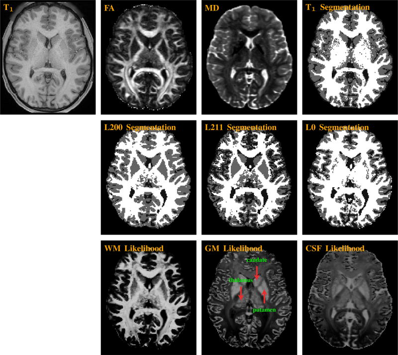
Figure 1 indicates that the segmentation result of the proposed method, L200, resembles very closely to that produced using the T₁-weighted image with the FSL FAST algorithm [20]. L211 produces WM segmentation result that is similar to L200, but underestimates GM. Note that these two methods are able to separate the deep GM structures, such as caudate and putamen, from the surrounding WM. The segmentation of the thalamus is more challenging because it is a mixture of GM and WM (see likelihood maps in the bottom row of Fig. 1).

Fig. 1.

(Top) T₁-weighted, fractional anisotropy (FA), mean diffusivity (MD), and T₁ segmentation images. (Middle) Segmentation maps given by L200 (proposed), L211, and L0. (Bottom) Likelihood maps for WM, GM, and CSF given by L200.

Quantitative

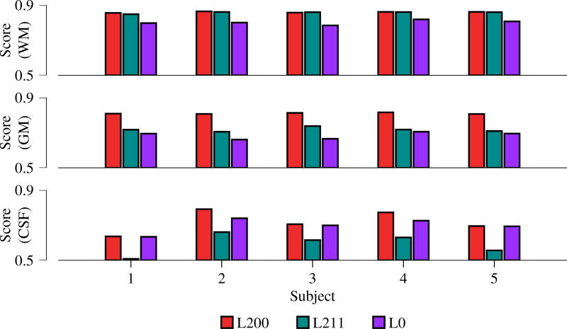
Figure 2 shows the Dice scores for WM-GM-CSF segmentation of 5 subjects from the HCP data repository, confirming again that the proposed method produces segmentation results that agree most with segmentation based on T₁-weighted images. The average Dice scores for L200/L211/L0 are 0.8603/0.8581/0.8019 (WM), 0.8105/0.7177/0.6844 (GM), and 0.7204/0.5941/0.6985 (CSF).

Fig. 2.

Accuracy of segmentation outcomes evaluated based on Dice score using T₁ segmentations as the ground truth.

Smoothing

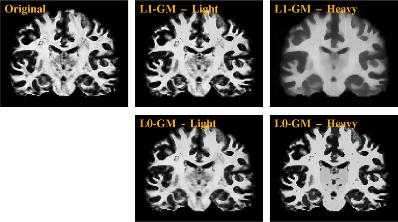
Figure 3 shows the effects of smoothing with different strengths using L1-GM and L0-GM. The results confirm that despite the increased smoothing strength, L0-GM can still preserve edges effectively. On the other hand, L1-GM blurs the edges when the smoothing strength is increased.

Fig. 3.

Effects of light and heavy smoothing using L1-GM and L0-GM. The WM, GM, CSF posterior probability maps are smoothed concurrently. However, due to space limitation, only the WM probability maps are shown here.

4 Conclusion

In this paper, we have presented a tissue segmentation method that works directly with diffusion MRI data. We demonstrated that the proposed method is able to produce segmentation results that are in good agreement with the more conventional T₁-based segmentation. We also showed that diffusion MRI provides additional information for segmentation of deep gray matter structures, complementary to T₁-weighted imaging, where image contrast in this region is typically low. Future research will be directed to further improving the segmentation of deep gray matter.

References

- 1.Liu T, Li H, Wong K, Tarok A, Guo L, Wong ST. Brain tissue segmentation based on DTI data. NeuroImage. 2007;38(1):114–123. doi: 10.1016/j.neuroimage.2007.07.002. [DOI] [PMC free article] [PubMed] [Google Scholar]
- 2.Awate SP, Zhang H, Simon TJ, Gee JC. Multivariate segmentation of brain tissues by fusion of MRI and DTI data; IEEE International Symposium on Biomedical Imaging (ISBI); 2008. pp. 213–216. [Google Scholar]
- 3.Lenglet C, Rousson M, Deriche R. A statistical framework for DTI segmentation; International Symposium on Biomedical Imaging; Apr, 2006. pp. 794–797. [Google Scholar]
- 4.Daducci A, Ville DVD, Thiran JP, Wiaux Y. Sparse regularization for fiber ODF reconstruction: From the suboptimality of ℓ2 and ℓ1 priors to ℓ0. Medical Image Analysis. 2014;18:820–833. doi: 10.1016/j.media.2014.01.011. [DOI] [PubMed] [Google Scholar]
- 5.Yap PT, Shen D. Spatial transformation of DWI data using non-negative sparse representation. IEEE Transactions on Medical Imaging. 2012;31(11):2035–2049. doi: 10.1109/TMI.2012.2204766. [DOI] [PMC free article] [PubMed] [Google Scholar]
- 6.Ramirez-Manzanares A, Rivera M, Vemuri BC, Carney P, Mareci T. Diffusion basis functions decomposition for estimating white matter intra-voxel fiber geometry. IEEE Transactions on Medical Imaging. 2007;26(8):1091–1102. doi: 10.1109/TMI.2007.900461. [DOI] [PubMed] [Google Scholar]
- 7.Candès EJ, Wakin MB, Boyd SP. Enhancing sparsity by reweighted ℓ1 minimization. Journal of Fourier Analysis and Applications. 2008;14(5):877–905. [Google Scholar]
- 8.Xu L, Lu C, Xu Y, Jia J. Image smoothing via ℓ0 gradient minimization. ACM Transactions on Graphics. 2011;30(5) [Google Scholar]
- 9.Yang J, Yin W, Zhang Y, Wang Y. A fast algorithm for edge-preserving variational multichannel image restoration. SIAM Journal on Imaging Sciences. 2009;2(2):569–592. [Google Scholar]
- 10.Tao M, Yang J. Technical report. Department of Mathematics, Nanjing University; 2009. Alternating direction algorithms for total variation deconvolution in image reconstruction. [Google Scholar]
- 11.Wright J, Yang AY, Ganesh A, Sastry SS, Ma Y. Robust face recognition via sparse representation. IEEE Transactions on Pattern Analysis and Machine Intelligence. 2009;31(2):1–18. doi: 10.1109/TPAMI.2008.79. [DOI] [PubMed] [Google Scholar]
- 12.Rudin LI, Osher S, Fatemi E. Nonlinear total variation based noise removal algorithms. Physica D. 1992;60:259–268. [Google Scholar]
- 13.Jeurissen B, Tournier JD, Dhollander T, Connelly A, Sijbers J. Multi-tissue constrained spherical deconvolution for improved analysis of multi-shell diffusion MRI data. NeuroImage. 2014 doi: 10.1016/j.neuroimage.2014.07.061. [DOI] [PubMed] [Google Scholar]
- 14.Simon N, Friedman J, Hastie T, Tibshirani R. A sparse-group lasso. Journal of Computational and Graphical Statistics. 2013;22(2):231–245. [Google Scholar]
- 15.Yap PT, Zhang Y, Shen D. Diffusion compartmentalization using response function groups with cardinality penalization. Medical Image Computing and Computer-Assisted Intervention. 2015 doi: 10.1007/978-3-319-24553-9_23. [DOI] [PMC free article] [PubMed] [Google Scholar]
- 16.Blumensath T, Davies ME. Iterative thresholding for sparse approximations. Journal of Fourier Analysis and Applications. 2008;14(5–6):629–654. [Google Scholar]
- 17.Lu Z. Iterative hard thresholding methods for ℓ0 regularized convex cone programming. Mathematical Programming. 2013:1–30. [Google Scholar]
- 18.Boyd S, Parikh N, Chu E, Peleato B, Eckstein J. Distributed optimization and statistical learning via the alternating direction method of multipliers. Foundations and Trend in Machine Learning. 2010;3(1):1–122. [Google Scholar]
- 19.Essen DCV, Smith SM, Barch DM, Behrens TE, Yacoub E, Ugurbil K. The WU-Minn human connectome project: An overview. NeuroImage. 2013;80:62–79. doi: 10.1016/j.neuroimage.2013.05.041. [DOI] [PMC free article] [PubMed] [Google Scholar]
- 20.Zhang Y, Brady M, Smith S. Segmentation of brain MR images through a hidden Markov random field model and the expectation-maximization algorithm. IEEE Transactions on Medical Imaging. 2001;20(1):45–57. doi: 10.1109/42.906424. [DOI] [PubMed] [Google Scholar]