Global Rate Variation in Bony Vertebrates

Abstract

This study investigated long-term substitution rate differences using three calibration points, divergences between lobe-finned vertebrates and ray-finned fish, between mammals and sauropsids, and between holosteans (gar and bowfin) and teleost fish with amino acid sequence data of 625 genes for 25 bony vertebrates. The result showed that the substitution rate was two to three times higher in the stem branches of lobe-finned vertebrates before the mammal-sauropsid divergence than in amniotes. The rate in the stem branch of ray-finned fish before the holostean-teleost fish divergence was also a few times higher than the holostean rate, whereas it was similar to or somewhat slower than the teleost fish rate. The phylogenetic relationship of coelacanth and lungfish with tetrapod was difficult to determine because of the short interval of the divergences. Considering the high rate in the stem branches, the divergences of coelacanth and lungfish from the stem branch were estimated as 408–427 Ma and 399–414 Ma, respectively, with the interval of 9–13 Myr. With the external calibration of the mammal-sauropsid split, the estimated times for ordinal divergences within eutherian mammals tend to be smaller than those in previous studies that used the calibration points within the lineage, with deeper divergences before the Cretaceous–Paleogene boundary and shallower ones after the boundary. In contrast the estimated times within birds were larger than those of previous studies, with the divergence between Galliformes and Anseriformes ∼80 Ma and that between Galloanserae and Neoaves 110 Ma.

Introduction

Variation of evolutionary rate among lineages has been observed in various taxonomic groups (Wu and Li 1985; Martin and Palumbi 1993; Duffy et al. 2008; Nabholz et al. 2008; Smith and Donoghue 2008; Eo and DeWoody 2010; Lanfear et al. 2010; Dornburg et al. 2012; Wertheim et al. 2012). Rate change in different time periods can also occur (e.g., Vermeij 1996; Aris-Brosou and Yang 2003; Smith and Donoghue 2008). The rate of molecular evolution is affected by mutation rate and the extent of genetic drift and natural selection, which are related with many factors in species biology such as diversification rate, life history, body size, and environments. Therefore, it is important to find out rate variation to clarify the relationship between mutation rate and natural selection and how molecular evolutionary rate is related with phenotypic evolution and speciation (e.g., Bromham 2009).

Another reason to investigate the rate of molecular evolution is that the rate variation can affect the estimation of divergence times (Bromham 2009; Lartillot et al. 2016; Bromham et al. 2018). Assumptions of the strict constant rate and varying rate sometimes generated disparate estimates of divergence times (e.g., Yoder and Yang 2000; Aris-Brosou and Yang 2003). Even though the methods that do not assume the strict constant rate are now available (e.g., Thorne et al. 1998; Sanderson 2002; Thorne and Kishino 2002; Drummond et al. 2006; Yang and Rannala 2006; Rannala and Yang 2007; Lartillot et al. 2009; Ronquist et al. 2012; Smith and O’Meara 2012; Tamura et al. 2012) and widely used, the estimates of divergence time are sensitive to the prior probability densities on calibration and rates (Welch and Bromham 2005; dos Reis and Yang 2013; Beaulieu et al 2015; dos Reis et al. 2015; Brown and Smith 2017) and not independent of choice of calibration points (e.g., Eme et al. 2014; Battistuzzi et al. 2015). Furthermore, the methods based on rate-smoothing (e.g., Sanderson 2002) are not expected to work well when there is extensive rate variation (Ho et al. 2005).

In this study, long-term rate variation in bony vertebrates and the effect on the time estimation are investigated using the data set that consists of amino acid sequences of 625 genes for 25 bony vertebrates and the three calibration points, divergences between lobe-finned vertebrates and ray-finned fish, between mammals and sauropsids, and between holosteans (gar and bowfin) and teleost fish.

This study also provides an opportunity to investigate the divergence time using external calibration points. In time estimation studies calibration points within lineages such as mammals (Springer et al. 2003; Bininda-Emonds et al. 2007; Meredith et al. 2011; dos Reis et al. 2012; O’Leary et al. 2013; Liu et al. 2017), birds (Jarvis et al. 2014; Prum et al. 2015), fish (Near et al. 2012), and angiosperms (Magallon et al. 2015) were often used. In these studies, a large number of species were included and a number of calibration points were set for estimating divergence times. However, many of the fossil records used for minimum ages for nodes can be affected by uncertainty of fossil assignment to lineages and incomplete fossil preservation (Smith and Peterson 2002; O’Reilly et al. 2015; Brown and Smith 2017) and choice of the calibration points affects the time estimates (Mitchell et al. 2015). This study, investigating the divergence times within mammals, sauropsids, and ray-finned fish, gives a complement to the previous time estimation studies, less subjected to these problems than the studies using internal calibration points.

In addition, the timing of divergences of orders of eutherian mammals and modern birds is particularly of interest because it has been controversial due to the scarcity of fossils in the Cretaceous Period (e.g., Foley et al. 2016 for mammals and Ksepka and Phillips 2015 for birds). Molecular studies supported the divergences of eutherian orders took place before the Cretaceous–Paleogene (K–Pg) boundary (66 Ma; Springer et al. 2003; Meredith et al. 2011; Bininda-Emonds et al. 2007; dos Reis et al. 2012; Liu et al. 2017), whereas paleontological records supported occurrence of the divergences after the K–Pg boundary (Archibald and Deutschman 2001; Asher 2005; Wible et al. 2007). Similarly, although fossil records indicate that only several basal bird lineages were in the Cretaceous (Ksepka and Phillips 2015), most of molecular studies supported diversification of major avian orders before the K–Pg boundary (e.g., Cooper and Penny 1997; Kumar and Hedges 1998; Brown et al. 2008; Pacheco et al. 2011; Haddrath and Baker 2012) except for recent genome-scale studies (Jarvis et al. 2014; Prum et al. 2015). By applying different rates within the lineages to time estimation, the rate changes within the lineages are also investigated.

Materials and Methods

Sequence Data and Estimation of Branch Lengths

The amino acid sequence data for 28 species of jawed vertebrates (fig. 1 and supplementary tables S1 and S2, Supplementary Material online) that consist of 651 genes with 185,280 amino acid sites compiled by Takezaki and Nishihara (2017) were used. Partitioning the data can reduce underestimation and enhance the precision of estimated branch lengths (Duchêne and Ho 2014; Angelis et al. 2018). Therefore, the branch lengths were estimated for partitions obtained by PartitionFinder 1.1 (Lanfear et al. 2012) and the averages were taken by weighting them with the number of sites. The search using PartitionFinder by BIC criterion generated 24 partitions (16 for JTT model, Jones et al. 1992 or JTT with amino acid frequencies estimated from the data (F), and 8 for LG, Le and Gascuel 2008 or MTMAM, Yang et al. 1998 +F under the assumption of rate variation across sites following the gamma distribution [G]) (supplementary table S1, Supplementary Material online). The branch lengths were estimated for each partition fixing the tree topology (fig. 1; Takezaki and Nishihara 2017) with the substitution model obtained by the PartitionFinder (supplementary table S1, Supplementary Material online) under the assumption of rate variation across sites following the gamma distribution with 8 discrete categories (G8) using codeml in PAML 4.9e (Yang 2007). The option of “Small_Diff” in codeml was set to 0.5 × 10⁻⁸ for the branch length estimation to facilitate the accuracy. Four partitions with a long terminal branch leading to a single species were excluded for further analyses (supplementary table S1, Supplementary Material online). In the final sequence data set used the total numbers of genes and amino acid sites were 625 and 178,984, respectively, with no missing data. The sequence data are available from the author upon request.

Fig. 1.

—Phylogenetic tree of 28 vertebrate species. The tree topology is from Takezaki and Nishihara (2017). The branch lengths were estimated by the maximum likelihood method for each of 24 partitions obtained by PartitionFinder with BIC criterion and weighted averages were taken by excluding four partitions in which a single species had a long terminal branch (see Materials and Methods). Cartilaginous fish was used as outgroup. The numbers that follows N (N29–N54) are those given to internal nodes. The red circles indicate the three nodes used as calibration points in this study.

In the preliminary analysis GTR model was also used for computation of branch lengths. The branch lengths were about up to ∼10% longer than those estimated by using the substitution models by PartitionFinder (supplementary tables S3 and S4, Supplementary Material online). However, the estimated times were mostly a few percent different from those using the substitution models suggested by PartitionFinder (data not shown). Therefore, the latter estimates of branch lengths were used for the analyses. The standard errors of the branch lengths were obtained by the curvature method, available as output of codeml. The average branch lengths from a node to the tips of the tree were obtained by computing the height of a node by repeatedly taking an average of the lengths of two descendant branches from tips toward the ancestral nodes. The rate on a branch was calculated as r = b/t where r, b, t are the rate, length and time length for the branch. In the time estimation in which the ratio of branch lengths is involved such that b1/r = (b1/b) × t, where b1 is length of a branch or a set of branches for which the time length is estimated for, the standard error was calculated by the delta method with approximation of the variance by Taylor expansion (e.g., Kendall and Stuart 1977) assuming the normal distribution for branch lengths. The first order Taylor expansion of a function of random variables x and y, f(x, y) is

$${f\left(x,y\right)\approx f\left({\mu }_x,\mathrm{}{\mu }_y\right)+f}_x^{\mathrm{\text{'}}}\left(x-{\mu }_x\right)+f_{y\mathrm{}}^{\mathrm{\text{'}}}\left(x-{\mu }_x\right),$$

where µ_x and µ_y are means of x and y, respectively. Then, variance of f(x, y), $Var\left(f\left(x,y\right)\right)=E\left\{{(f\left(x,y\right)-E(f\left(x,y\right))}^2\right\}$, can be approximated as

$$Var\left(f\left(x,y\right)\right)\approx {{E[f\left({\mu }_x,{\mu }_y\right)+f}_x^{\mathrm{\text{'}}}\left(x-{\mu }_x\right)+f_{y\mathrm{}}^{\mathrm{\text{'}}}\left(x-{\mu }_x\right)-f\left({\mu }_x,{\mu }_y\right)]}^2={\left[f_x^{\mathrm{\text{'}}}\left({\mu }_x,{\mu }_y\right)\right]}^{2}Var\left(x\right)+2f_x\left({\mu }_x,{\mu }_y\right)f_y\left({\mu }_x,{\mu }_y\right)\mathrm{C}\mathrm{o}\mathrm{v}\left(\mathrm{x},\mathrm{}\mathrm{y}\right)+{\left[f_y^{\mathrm{\text{'}}}\left({\mu }_x,{\mu }_y\right)\right]}^{2}Var\left(y\right)$$

In the phylogenetic tree used (fig. 1), the relationship of elephant (Afrotheria), armadillo (Xenarthra) and the other eutherian mammals [Boreoeutheria (Boreotheria)] is not established (Foley et al. 2016). The sister relationship of elephant and armadillo (fig. 1) was supported by previous studies such as Springer et al. (2003), Song et al. (2012), and Liu et al. (2017), but the earlier divergence of Afrotheria than Xenarthra was also supported by other studies (Nishihara et al. 2007; McCormack et al. 2012; Romiguier et al. 2013). Studies of rare genomic changes such as retroposon insertions revealed rapid divergences of Afrotheria, Xenarthra and Boreoeutheria in a narrow evolutionary time period (Churakov et al. 2009; Nishihara et al. 2009). The branch lengths were also estimated by assuming the other two possible tree topologies, but the lengths of the branches that connect these lineages were virtually the same, so the effect of these relationships on the time estimation would be small considering the short branches connecting them (Yang 1995; Yoder and Yang 2000).

In our previous studies (Takezaki and Nishihara 2016, 2017) the statistical support was not high for the relationship of stickleback, pufferfish and the other teleost fish. However, the sister relationship of stickleback and pufferfish (fig. 1) is consistent with other studies on fish phylogeny (e.g., Near et al. 2012; Broughton et al. 2013).

Fossil Calibration

To examine long-term rate variation in bony vertebrates, three calibration points were used for calculation of the evolutionary rate: 1) the split of ray-finned fish and lobe-finned vertebrates (N29 in fig. 1; minimum 420.7 million years ago [Ma], soft maximum 444.9 Ma), 2) the split of mammals and sauropsids (N33) (min. 318 Ma, soft max. 332.9 Ma), and 3) the split of teleost fish and holosteans (gar and bowfin; Holostei) (N45) (min. 250 Ma, soft max. 331 Ma). The minimum and soft maximum fossil ages were taken from Benton et al. (2015).

The fossil ages of the splits are not free from uncertainty (e.g., Muller and Reisz 2005). However, the split (1) is well constrained by the split of bony vertebrates and cartilaginous fish (min. 420.7 Ma, soft max. 468.4 Ma) and the split of tetrapod from coelacanth and lungfish (min. 408 Ma, soft max. 427.9 Ma). The fossil age of the split (2) is also considered to be well constrained by the first appearance of tetrapods and amniotes and less subjected to underestimation than those within mammals and birds (Hedges et al. 1996; Kumar and Hedges 1998). Although the minimum and maximum fossil ages of the split (3) have a large difference, I used them to see the rate difference in ray-finned fish.

The divergences at the stem branch of lobe-finned vertebrates (N30–N32) occurred within a relatively short time period of 87.8–127 Myr. The phylogenetic relationship of coelacanths, lungfishes, and tetrapods had been controversial due to the short time interval of the divergences and only recently the sister relationship of lungfish and tetrapods was strongly supported with the use of genome-scale data (Amemiya 2013; Liang et al. 2013; Chen et al. 2015; Irisarri and Meyer 2016; Takezaki and Nishihara 2016, 2017). The divergence times within mammals and birds are still debated as stated in Introduction. Therefore, in this study I focused on the use of the three calibration points and variation of the long-term rates.

Time Estimation by Bayesian Method

MCMCTree in PAML 4.9e (Yang 2007) was used to obtain Bayesian time estimates. Following the instruction of MCMCTree tutorials in PAML package, a method of approximate likelihood calculation (dos Reis and Yang 2011) was used. First, the Hessian matrix was generated by codeml for each partition by adjusting “rgene_gamma” parameters with average rates calculated from the estimated branch lengths. Then, the Hessian matrices of different partitions were concatenated and used as input of MCMCtree for divergence time estimation.

The time estimates were carried out under the relaxed-clock model for autocorrelated-rates model (ARM) and independent-rates model (IRM; Rannala and Yang 2007). The parameters of iterations of MCMC (Markov chain Monte Carlo) were set as burnin = 400,000, sampfreq = 5, nsample = 1,000,000. Using Tracer v1.6 (Rambaut et al. 2013), the effective sampling sizes (ESSs) were computed. ESSs were >200 for all the nodes, indicating that the estimation of the posterior distributions of the node ages is not poor (Susko 2008; Drummond et al. 2012). Lower and upper bounds of fossil calibration were given to the three calibration points mentioned above. The left tail probabilities (p_L) of the Cauchy distribution for divergence times were set to 10⁻³⁰⁰, and the right tail probabilities (p_U) were set to 0.05 and 10⁻³⁰⁰ in all calibration points (see the section of mcmctree in PAML manual). RootAge was set as <6.0 in the unit of 100 My. All the other parameters were set as default values. Because the results of two independent runs were very similar (data not shown), only the averages of two runs are shown (supplementary table S5, Supplementary Material online). To see fit of the ARM and the IRM to the data, Bayes factor, which is a ratio of a likelihood of one hypothesis over a likelihood of the other (Kass and Raftery 1995), was calculated.

Results

Rate Variation among the Lineages

To see among-lineage rate variation and rate differences in different time periods in bony vertebrates, substitution rates (the number of substitutions per site per 10¹⁰ years) from the three nodes (N29, N33, N45) (R29, R33, R45) of the phylogenetic tree (fig. 1) are calculated, by dividing the branch lengths from the nodes to tips of the tree (supplementary table S6, Supplementary Material online) by the fossil ages of the nodes (see Materials and Methods). Rates between N29 and N33 and between N29 and N45 (R29–33 and R29–45) are calculated, by dividing the sums of the branch lengths between the two nodes by their time intervals (fig. 2 and supplementary table S7, Supplementary Material online). The three nodes correspond to the divergences between lobe-finned vertebrates and ray-finned fish (N29, 427–444.9 Ma), between mammals and sauropsids (N33, 318–332.9 Ma) and between teleost fish and holosteans (gar and bowfin) (N45, 250–331 Ma). R29s are calculated for all bony vertebrates, R33s for amniotes, and R45s for ray-finned fish.

Fig. 2.

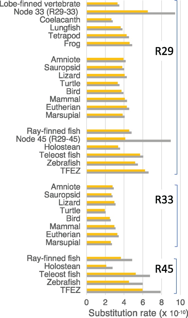
—The substitution rates estimated by setting nodes 29, 33, 45 (N29, N33, N45) as calibration points (R29, R33, R45). Orange bars and gray bars indicate rates assuming minimum and maximum ages for the nodes, respectively. TFEZ: teleost fish excluding zebrafish. Holostean: gar and bowfin.

As can be seen in the branch lengths of the tree (fig. 1 and supplementary table S6, Supplementary Material online), teleost fish have the highest R29 (5.17–5.47 for zebrafish and 6.24–6.60 for teleost fish excluding zebrafish [TFEZ]) and coelacanth has the lowest (2.64–2.79). Lungfish R29 (3.62–3.82) is 25% higher than that of coelacanth. Among tetrapods, R29 for frog (4.60–4.86) is higher than those for amniotes (3.32–4.55). In the ray-finned fish, holostean R29 (3.37–3.56) is 30–50% slower than those of teleost fish.

In the phylogenetic tree (fig. 1), cartilaginous fish were used as outgroup to determine the root of the ingroup (bony vertebrates) (N29). The branch lengths from the root to cartilaginous fish are shorter (0.08–0.11) than any of those to bony vertebrates (supplementary table S4, Supplementary Material online). Although the position of the root on the branch connecting cartilaginous fish and bony vertebrates is not determined, it suggests that the evolutionary rate of cartilaginous fish is slower than those of bony vertebrates, consistent with a previous study (Venkatesh et al. 2014).

Rates and Time Estimates at the Stem-Branch of Lobe-Finned Vertebrates

By assuming the time interval between N29 and N33 as 87.8–127 My from the fossil ages of the two nodes, the rate for this stem branch (R29–33) (6.64–9.43) becomes about three times as high as R33s of amniotes. If this rate is assumed at the stem branch, the rates for coelacanth, lungfish, and frog after divergence from the stem branch at the external branch become 10–15% smaller than their R29s (rate E and F in supplementary table S7, Supplementary Material online). Because of this high rate at the stem branch, amniote R33s (1.95–3.41) are 25–40% smaller than their R29s and comparable to R29s of coelacanth and lungfigh (fig. 2 and supplementary table S7, Supplementary Material online).

In order to see if the high rate estimated for the stem branch (R29–33) fits the fossil ages, divergence times at the stem branches of lobe-finned vertebrates between N29 and N33 are obtained using the R29–33. They are close matches to the fossil ages (fig. 3 and supplementary table S8, Supplementary Material online). With these estimates, after the divergence between lobe-finned vertebrates and ray-finned fish (N29), it took 13–18 My to coelacanth divergence (N30), 9–13 My to lungfish divergence (N31), 41–50 My (N32) to frog divergence, and 25–37 My (N33) to the divergence between mammals and sauropsids (supplementary table S8, Supplementary Material online). It should be noted that with the use of R29s of coelacanth and lungfish which are one third to a half of R29–33, the time interval between N29 and N33 become about two to three times (200–300 My) as long as that indicated by the fossil records (supplementary table S8, Supplementary Material online). Therefore, it is likely that the rate was high at the stem branch and slowdown occurred in the coelacanth and lungfish lineages after divergence.

Fig. 3.

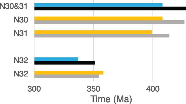
—The fossil ages and estimated times at the stem branch of by setting N29 and N33 as calibration points. Blue and black bars indicate minimum and maximum ages of fossil ages, respectively. Orange and gray bars indicate estimated times by assuming the minimum and maximum time intervals (87.8 and 128 My) between N29 and N33.

Rates and Divergence Times in Mammals, Sauropsids, and Ray-Finned Fish

Divergence times within mammals, sauropsids, and ray-finned fish are estimated by setting external calibration points, N33 for mammals and sauropsids (with the use of R33) and N29 and N45 for ray-finned fish (with the use of R29 and R45). It should be noted that with R29s for time estimation of mammals and sauropsids, which are >30% higher than R33s, the time estimates for the divergence of the two groups become about 200 Ma or more recent and those within these groups will be unrealistically small (not shown).

There are rate differences within the lineages such that eutherian rate is higher than marsupial rate in mammals, lizard rate higher than turtle and bird rates in sauropsids, and teleost fish rate higher than holostean rate in ray-finned fish (fig. 2 and supplementary table S7, Supplementary Material online). In the time estimation these different rates are used to see how they affect the time estimates and rate changes within the lineages are investigated by comparing the estimated times with fossil records.

Divergence Times and Rates within Mammals

Divergence times within mammals estimated with R33 are shown in figure 4 and supplementary table S10, Supplementary Material online. R33s for eutherians (3.41–3.26) are ∼25% higher than those for marsupials (2.70–2.58; fig. 2 and supplementary table S7, Supplementary Material online). The divergence times within mammals are estimated, by assuming the marsupial R33 and the eutherian R33 at the branch between N33 and N34 (divergence between eutherians and marsupials). With the marsupial R33 at the branch between N33 and N34, the times within eutherians (N35–N38) are obtained by re-estimating the eutherian rate after divergence at N34 (rate G in supplementary table S7, Supplementary Material online), whereas with the eutherian R33 at the branch between N33 and N34, the time within marsupials (N39) is computed by re-estimating the marsupial rate (rate H in supplementary table S7, Supplementary Material online). Similarly, in the following, the time estimates within sauropsids and ray-finned fish are obtained by re-estimating the rates when the rate for different species or group is assumed at the ancestral branch (supplementary tables S10 and S11, Supplementary Material online).

Fig. 4.

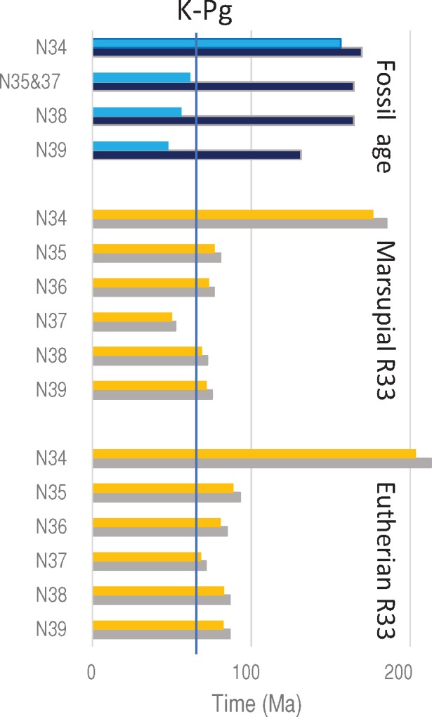
—The fossil ages and estimated times within mammals by setting N33 as a calibration point. Blue and black bars indicate minimum and maximum ages of fossil ages, respectively. Orange and gray bars indicate estimated times by setting the minimum and maximum fossil ages of N33 as calibration points. The solid vertical line indicates K–Pg boundary (66 Ma).

Assuming the eutherian R33 between N33 and N34, the estimates for the divergence between marsupials and eutherians (N34) appears somewhat large (204–213 Ma) compared with the fossil age (156–170 Ma) and those within eutherians (N35–N38) (68–93 Ma) are all before the K–Pg boundary (66 Ma). Assuming the marsupial R33 between N33 and N34, the time for N34 (177–185 Ma) is closer to the fossil age and the estimates within eutherians became 10–20 My smaller (50–81 Ma), which are closer to or even younger than the K–Pg boundary (fig. 4). In this case, however, the time estimate for N37 (50.0–52.4 Ma) is smaller than the fossil age (61.6–164.6 Ma). Therefore, it is unlikely that the rate at the ancestral branch (N33–N34) was as slow as the marsupial R33.

Divergence Times and Rates within Sauropsids

Divergence times within sauropsids estimated with R33s are shown in figure 5 and supplementary table S10, Supplementary Material online. R33 for lizard (2.95–3.09) is higher than those for birds (2.47–2.59), and turtle (1.95–2.04; fig. 2 and supplementary table S7, Supplementary Material online). Correspondingly, time estimates with the lizard R33 at the branches between N33 and N41 (turtle divergence) are larger than those with the bird and turtle R33s (fig. 5 and supplementary table S10, Supplementary Material online). The estimates with the lizard R33 for the lizard divergence (N40) (271–284 Ma) and the turtle divergence (N41) (242–253 Ma) are good matches to the fossil ages of the nodes (255.9–295.9 Ma), whereas those with the turtle R33 (203–256 Ma) and that for N41 (228–238 Ma) with the bird R33 become much smaller than the fossil ages (fig. 5 and supplementary table S10, Supplementary Material online). This result suggests that the rate at the ancestral branches between N33 and N41 was as high as the lizard R33 and slowdown of the rate occurred in the turtle and bird lineages. If we assume the lizard R33 at the ancestral branch(es), the rate at the turtle lineage become 16% smaller (1.64–1.71) than the turtle R33 and the rate at the bird lineage (2.32–2.43) 6% smaller than the bird R33 (rate I in supplementary table S7, Supplementary Material online).

Fig. 5.

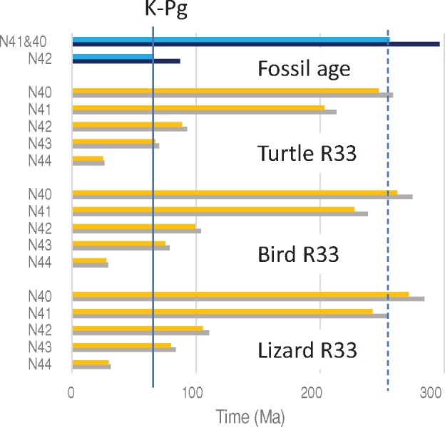
—The fossil ages and estimated times within sauropsids by setting N33 as a calibration point. Blue and black bars indicate minimum and maximum ages of fossil ages, respectively. Orange and gray bars indicate estimated times using the minimum and maximum fossil ages of N33 as calibration points. The solid vertical line indicates K–Pg boundary (66 Ma). The dotted vertical line indicates the minimum fossil age of N40 and N41.

By assuming the lizard R33 at the branches between N33 and N41, time estimates for the divergences between Neoaves (flycatcher) and Galloanserae (chicken, turkey and duck) (N42), between Anseriformes (duck) and Galliformes (chicken and turkey) (N43) and between chicken and turkey (N44), become 106–110 Ma, 80–83.6 Ma, and 29.5–30.9 Ma, respectively. The first two estimates are well before the K–Pg boundary (fig. 5 and supplementary table S10, Supplementary Material online).

Time Estimates and Rates for Ray-Finned Fish

Divergence times within ray-finned fish, by using R29s and R45s for zebrafish and TFEZ in figure 6 and supplementary table S11, Supplementary Material online. Whereas the zebrafish rates (5.17–5.47 for R29s and 4.52–5.99 for R45s) are slightly smaller than the TFEZ rates (6.24–6.60 for R29s and 5.96–7.89 for R45s), the holostean rates (3.37–3.56 for R29s and 2.10–2.78 for R45s) are much smaller (59–65% for R29 and 40–46% for R45) than those of zebrafish and TFEZ. The estimates for the divergence between holosteans and teleost fish (N45) with the holostean R29s are much smaller than the fossil age, and those within the teleost fish lineage (N46–N51) also tend to be smaller than the fossil ages with the holostean R29s and R45s (not shown). In contrast the time estimates with the zebrafish and TFEZ rates are within the range of or larger than the fossil ages, although time estimates with the zebrafish R29s are slightly smaller than those with the TFEZ R29s. The estimates with zebrafish and TFEZ R45s become slightly smaller or larger than those with their R29s, depending whether the rate was calibrated with the minimum or maximum of the fossil age of N45, but they are also consistent with the fossil ages.

Fig. 6.

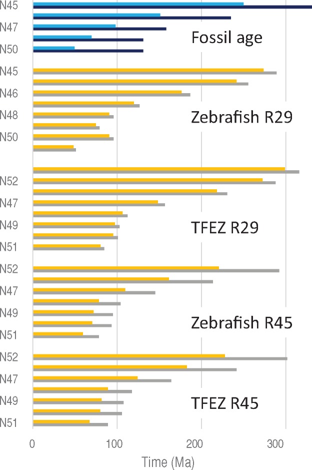
—The fossil ages and estimated times in ray-finned fish by setting N29 and N45 as calibration points. Blue and black bars indicate minimum and maximum ages of fossil ages, respectively. Orange and gray bars indicate estimated times.

Similarly to R33s for amniotes, R45s for holosteans (2.10–2.78) are 20–40% smaller than their R29s (fig. 2 and supplementary table S7, Supplementary Material online). Correspondingly, by assuming the time intervals of the fossil ages of N29 and N45 (89.7–195 My), the rate between the two nodes (R29–45) (4.12–8.96) becomes two to three times higher than the holostean R45s. In contrast R45s of zebrafish and TFEZ are about 10% larger than their R29s estimated with the minimum age of N45 (250 Ma) but those with the maximum age (331 Ma) are 5–20% smaller (4.52 for zebrafish and 5.96 for TFEZ) than their R29s. Accordingly, the R29–45 with the minimum time interval (89.7 My) is 10–30% higher than R45 of TFEZ and zebrafish, but that with the maximum interval (195 My) is 50–10% smaller (fig. 2 and supplementary table S7, Supplementary Material online). These results suggest that slowdown of the rate occurred in the holostean lineage after divergence from the stem branch, but the rate in the teleost fish could have become either higher or lower than that at the stem branch, depending on whether the minimum or maximum time interval is assumed for the stem branch.

Discussion

High Rate in the Stem Lineages and Slowdown of the Rates in the Peripheral Branches in Bony Vertebrates

This study estimated amino acid substitution rates using 625 orthologous genes of 25 bony vertebrates using the fossil ages of the three nodes (N29, N33, and N45) corresponding to the divergences of lobe-finned vertebrates and ray-finned fish, mammals and sauropsids, and holosteans and teleost fish. In the results the rate at the stem branch of lobe-finned vertebrates (R29–33) was higher than those of coelacanth, lungfish, and frog, which diverged from the stem lineage, and amniotes after divergence at N33 (R33) (fig. 2 and supplementary table S7, Supplementary Material online). The rate at the stem branch of ray-finned fish (R29–45) was also much higher than that of holosteans (R45). The teleost fish R45 was higher than that in the stem branch (R29–45) when the minimum fossil age (250 Ma) was assumed for the divergence between holosteans and teleost fish (N45). However, with the maximum fossil age for N45 (331 Ma), which gives a narrow interval between N29 and N45 (87.8 My), the rate at the stem branch became higher than that of teleost fish (fig. 2 and supplementary table S7, Supplementary Material online). Therefore, it is possible that slowdown of the rate occurred even in the teleost fish. The high rates at the stem branches and the slowdown at the peripheral branches may be related with such factors as high diversification rate at the stem branches and increase of body size at peripheral branches. Note that the high diversification rate at the stem branch of lobe-finned vertebrates was suggested by fossil records indicating that lobe-finned fishes were dominant in number of species for many million years in the Paleozoic (∼540–250 Ma) and many lineages existed, although at the end of the Paleozoic only coelacanths, lungfishes and tetrapods remained and ray-finned fish became dominant in water (Clack 2002). However, it needs future investigation because the evolutionary rate is a complex function of many factors involved in the species diversification rate (Eo and DeWoody 2010; Lanfear et al. 2010; Duchene and Bromham 2013), life history (e.g., generation time [Li et al. 1996; Bromham et al. 2002; Smith and Donoghue 2008; Thomas et al. 2010], life span [Nabholz et al. 2008; Welch et al. 2008]), body size (Bromham 2002; Wollenberg et al. 2011; Figuet et al. 2016), and environment (e.g., Davies et al. 2004; Wright et al. 2006; Lourenco et al. 2013).

There are uncertainties associated with the fossil ages used in this study. However, considering the fossil ages of such divergences as those between cartilaginous fish and bony fish (420–468 Ma) or between lobe-finned fish and tetrapods (408–427.9 Ma), which occurred before or after the divergence between cartilaginous fish and bony fish (N29), change of the age of N29 (420.7–444.9 Ma) would be limited to a narrow range (fossil ages are from Benton et al. 2015). This is also the case for the age of divergence of mammals and sauropsids (N33) (318–332.9 Ma) that took place after the divergence between amphibians and amniotes (337–351 Ma) and before the divergence of lizard, turtle, and birds (255.9–295.9 Ma). The rate of the stem branch of lobe-finned vertebrates (R29–R33) was two to three times higher than R33, by assuming the time interval (87–123 My). Therefore, even if the actual ages of N29 and N33 could be older than the assumed age, the conclusion that the R29–R33 at the stem branch was higher than R33 at peripheral branches would not change.

It should be also noted that the high rate at the stem branch is not an artifact of underestimation of branch lengths. If inappropriate substitution models are used for branch length estimation, branch lengths could be underestimated. However, in such a case lengths of deep branches would be more underestimated than those of shallow ones. Then, the rates in deep branches would become smaller relative to the rates at shallow branches.

Rate Variation in Different Time Periods and Molecular Time Estimation

With the use of molecular sequence data much older divergence times were often generated than the fossil records (Pagel 1999; Benton and Ayala 2003; Ksepka and Phillips 2015). A good example is the time of early animal evolution for which reliable fossils are scarce before the Cambrian Period (541–485 Ma; Bromham and Hendy 2000; Hug and Roger 2007; Lee et al. 2013; Eme et al. 2014). Extrapolation of rates at shallow branches often led to large estimates at deep nodes in early studies (e.g., >1200 Ma [Wray et al. 1996; Bromham et al. 1998], 830 Ma [Gu 1998]; >970 Ma [Nei et al. 2001]). Using the relaxed-clock methods, in which the time estimates can be constrained by multiple calibration points, the estimates became relatively younger (∼600–1300 Ma; Douzery et al. 2004; Hedges et al. 2004; Petersen et al. 2004; Erwin et al. 2011; Dohrmann and Wörheide 2017).

However, in addition to the choice of calibration points the estimated times can vary due to the assumptions used in the analyses such as the time prior and the maximum for the root age and models of rate change among branches (e.g., independent or autocorrelated; Rannala and Yang 2007) in the relaxed-clock method (e.g., Ho et al. 2005; Warnock et al. 2012, 2014; Battistuzzi et al. 2015; dos Reis et al. 2015; Dohrmann and Wörheide 2017; see also the section of Bayesian Time Estimates below). Therefore, understanding the pattern of rate variation in different time periods is necessary to improve the modeling in time estimation. Clear evidence of the high rates at the stem branches of lobe-finned vertebrates in this study contributes to the improvement in the time estimation method.

Whole Genome Duplication and the High Rate of Teleost Fish

It has been recognized that genes of teleost fish evolve faster than those of mammals (e.g., Robinson-Rechavi and Laudet 2001; Jaillon et al. 2004; Amemiya 2013; Venkatesh et al. 2014). In this study rates of teleost fish (R45) were also higher than those for mammals (R33). The whole genome duplication that occurred at the common ancestor of teleost fish (TGD) was thought to have facilitated the high rate of teleost fish (Crow and Wagner 2006; Braasch et al. 2016). However, a previous study showed that teleost fish genes, whether they are duplicates or singletons, generally have higher nonsynonymous to synonymous substitution rate ratio (Ka/Ks) than their orthologs in mammals (Brunet et al. 2006). In addition, one of the paralogs of >70–80% of the duplicated genes at TGD was already lost in the present teleost fish genomes (e.g., Brunet et al. 2006; Braasch and Postlethwait 2012; Inoue et al. 2015) and most of the losses occurred rapidly within 60 My after TGD (Inoue et al. 2015). These results suggest that the high rate of teleost fish was not due to TGD and that it is possible that the rate of ray-finned fish was high even before the divergence of teleost fish and holosteans. It is consistent with this study that R29–45 was higher than mammalian R33s for both the minimum and maximum time intervals between N29 and N45 and that slowdown of the rate possibly occurred in the teleost lineage if the maximum of the fossil age is assumed for N45.

Slow Rate of Coelacanth

The branch length from the root of the tree is the shortest for coelacanth among the bony vertebrates (fig. 1 and supplementary table S4, Supplementary Material online, see also Amemiya 2013; Braasch et al. 2016). Accordingly, the average rate from the root (R29) was the lowest for coelacanth (supplementary table S7, Supplementary Material online and see Amemiya 2013; Braasch et al. 2016). However, the fast rate on the stem branches of lobe-finned vertebrates and ray-finned fish was taken into accounts, the rates of birds (2.32–2.43, rate I in supplementary table S7, Supplementary Material online) and marsupials (2.30–2.41, rate H in supplementary table S7, Supplementary Material online) (R33), as well as that of holosteans (2.40–2.54, rate M in supplementary table S7, Supplementary Material online) (R45) became similar to or lower than the rate of coelacanth (2.45–2.56, rate E and F in supplementary table S7, Supplementary Material online). The rate of turtle (1.64–1.71, rate I in supplementary table S7, Supplementary Material online) (R33) was the lowest (supplementary table S7, Supplementary Material online) among all examined in this study.

Interval of Coelacanth and Lungfish Divergences and Incomplete Lineage Sorting (ILS)

The phylogenetic relationship among coelacanth, lungfish, and tetrapod was difficult to resolve because of the short internal branch between the divergences of coelacanth and lungfish and their long external branches. However, recent studies using the coelacanth genome data firmly determined that lungfish is closer to tetrapod than coelacanth (Amemiya 2013; Liang et al. 2013; Chen et al. 2015; Irisarri and Meyer 2016; Takezaki and Nishihara 2016, 2017). With this established tree topology, the interval of the divergences of coelacanth and lungfish was estimated as ∼10 My with the fast rate of the stem branch of lobe-finned vertebrates (R29–33) (supplementary table S8, Supplementary Material online). The population sizes of bony vertebrates generally appear relatively small (in the order of 10⁵ or smaller; Romiguier et al. 2014). Therefore, it is likely that the coalescence time of alleles (4N generations) is smaller than the interval of the coelacanth-lungfish divergence, so that the effect of ILS is small in the phylogenetic signals for coelacanth, lungfish, and tetrapod. In fact, in the phylogeny construction of coelacanth, lungfish and tetrapod, whether outgroup was highly divergent (teleost fish) or not (cartilaginous fish and holosteans) had a strong effect on the constructed tree topology and the effect of ILS appeared to be small (Takezaki and Nishihara 2016, 2017).

In contrast, at the root of the eutherian clade, the length of the internal branch connecting elephant (Afrotheria) and armadillo (Xenarthra) was ∼20% of that of the branch between the divergences of coelacanth and lungfish (supplementary table S3, Supplementary Material online). ILS has been considered to be a major source of difficulty in inferring mammalian phylogeny (e.g., McCormack et al. 2012; Song et al. 2012). Although a recent study indicated that the effect of ILS is small (∼0.12%) in the misleading signals of mammalian phylogenies (Scornavacca and Galtier 2017), a massive extent of ILS of retroposon insertions among Afrotheria, Xenarthra, and other eutherians (Boreoeutheria) has been observed (Churakov et al. 2009; Nishihara et al. 2009). Liu et al. (2017) also found that the coalescence analysis generated more congruent tree topologies than the concatenation analysis.

Divergence Times within Mammals and Sauropsids

In mammals the estimates of the divergences within eutherians were ∼70–90 Ma by assuming the eutherian rate (R33) at the ancestral branch before the eutherian-marsupial divergence and ∼50–80 Ma by assuming the marsupial rate. Previous studies that used the divergence of mammals and sauropsids (N33) as a calibration point, similarly to this study, provided older estimates for the divergences of eutherian groups (>100 Ma; Hedges et al. 1996; Kumar and Hedges 1998). However, the estimates of this study were close to or even younger than the estimates in previous studies that used calibration points within eutherians (80–90 Ma; Springer et al. 2003; Meredith et al. 2011; dos Reis et al. 2012). This result suggests the closeness of eutherian interordinal divergence to the K–Pg boundary (66 Ma) and favors that the ordinal divergence started in the Cretaceous and continued across the K–Pg boundary (trans-KPg model; Liu et al. 2017).

In mammals, time estimates assuming the eutherian R33 at the ancestral branch (N33–N34) were more likely than those assuming the marsupial R33. In addition, in the sauropsid lineage, it appeared likely that the rate was as high as the lizard rate (R33) at the ancestral branches before the turtle-bird split (N33–N41) and slowed down in the turtle and bird lineages, considering the old fossil ages of these nodes (N40 and N41) (255.9–296 Ma), in comparison to the time estimates by assuming the turtle and bird rates at the ancestral branch between N33 and N41. By assuming the lizard rate at the ancestral branch, the divergence between Gallloanserae (Galliformes [chicken and turkey] and Anseriformes [duck]) and Neoaves (Passeriformes [flycatcher]) became 106–110 Ma, and that between Galliformes and Anseriformes 80–84 Ma. These estimates are larger than those of previous studies that used within-lineage calibration points (∼90 Ma and ∼65 Ma in Jarvis et al. 2014 and ∼70 Ma and 55 Ma in Prum et al. 2015), in contrast to the estimates for mammals which were similar to or younger than those in these previous studies, although the previous study using the external calibration point (N33) generated a much larger estimate (112 Ma) for the divergence of Galliformes and Anseriformes (Kumar and Hedges 1998).

Bayesian Time Estimates

Time estimates by the Bayesian method with MCMCTree (Yang 2007) were carried out using the three nodes (N29, N33, N45) as the calibration points (supplementary table S4, Supplementary Material online) for the ARM and the IRM (Rannala and Yang 2007). The two values were used for the right tail probability (p_U) for the fossil calibration prior (p_U = 0.05 and 10⁻³⁰⁰) were used. The time estimates with p_U = 0.05 were larger than those with p_U = 10⁻³⁰⁰ at the majority of the nodes, as expected. However, the difference of the estimates with the two p_U values were small (<3 My for the ARM and <7 My for the IRM). Even in most of nodes of mammals for both the ARM and the IRM and amniotes for the ARM the estimates with p_U = 0.05 were smaller than those with p_U = 10⁻³⁰⁰.

The estimates with the ARM and the IRM were similar to each other at the stem branch of lobe-finned vertebrates (between N30 and N33), with the former being mostly slightly larger (<10 My) than the latter. In contrast the difference of the estimates with the ARM and the IRM were quite large within amniotes (27–64 My) with the former being higher than the latter and within ray-finned fish (4–51 My) with the former being smaller than the latter. Note that the IRM estimates were larger than the ARM estimates at the root of the whole tree including cartilaginous fish and at the root of bony vertebrates (N29) for p_U = 0.05.

In the result, the rates of ray-finned fish were generally higher than those of amniotes (supplementary table S7, Supplementary Material online). However, in the IRM the rates are assigned to all branches assuming a common distribution function with a mean of the average rate. Therefore, rates slower than the actual rates would be assigned to branches in ray-finned fish with fast rate and rates faster than the actual rates would be assigned to branches in amniotes. Because of this rate assignment with the IRM, the time estimates in ray-finned fish tend to be large, even in comparison to the time estimates of this study using the rates directly estimated with the branch lengths and the fossil age of the calibration points.

With the ARM, the rates are assigned to descendant branches assuming that they are a certain function of the rate at the ancestral branch (in MCMCTree the log-normal distribution). The rates appear to be correlated particularly in the branches nearby. However, the fit of IRM and ARM to data has been controversial (Drummond et al. 2006; Linder et al. 2011; Ho et al. 2015; Bromham et al. 2018). The extent of the correlation may not be the same in all over the tree (Ho et al. 2015; Lartillot et al. 2016). Therefore, the current implementation of the pattern of correlation of rates in the ARM may not be appropriate. The overall likelihood value for ARM was slightly lower than that for IRM (supplementary table S5, Supplementary Material online), but the values of the Bayes factor, a ratio of the likelihood values, were close to 1. So, there was no indication of which model fits better (Kass and Raftery 1995; Bromham et al. 2018) and it is difficult to decide a priori which model to be used in this case.

Supplementary Material

Supplementary data are available at Genome Biology and Evolution online.

Literature Cited

- Amemiya C., et al. , . 2013. The African coelacanth genome provides insights into tetrapod evolution. Nature 4967445:311–316. [DOI] [PMC free article] [PubMed] [Google Scholar]
- Angelis K, Alvarez-Cárretero A, dos Reis M, Yang Z.. 2018. An evaluation of different partitioning strategies for Bayesian Estimation of species divergence times. Syst Biol. 671:61–77. [DOI] [PMC free article] [PubMed] [Google Scholar]
- Archibald JD, Deutschman DH.. 2001. Quantative analysis of the timing of origin of extant placental orders. J Mamm Evol. 82:107–124. [Google Scholar]
- Aris-Brosou S, Yang Z.. 2003. Bayesian models of episodic evolution support a late Precambrian explosive diversification of the Metazoa. Mol Biol Evol. 2012:1947–1954. [DOI] [PubMed] [Google Scholar]
- Asher RJ. 2005. Stem Lagomorpha and the antiquity of Glires. Science 3075712:1091–1094. [DOI] [PubMed] [Google Scholar]
- Battistuzzi FU, Billing-Ross O, Murillo O, Filipski A, Kumar S.. 2015. A protocol for diagnosing the effect of calibration priors on posterior time estimates: a case study for the Cambrian explosion of animal phyla. Mol Biol Evol. 327:1907–1912. [DOI] [PMC free article] [PubMed] [Google Scholar]
- Beaulieu JM, O’Meara BC, Crane P, Donoghue MJ.. 2015. Heterogeneous rates of molecular evolution and diversification could explain the Triassic age estimate for angiosperms. Syst Biol. 645:869–878. [DOI] [PubMed] [Google Scholar]
- Benton M, Ayala FJ.. 2003. Dating the tree of life. Science 3005626:1698–1700. [DOI] [PubMed] [Google Scholar]
- Benton M, et al. , . 2015. Constraints on the timescale of animal evolutionary history. Palaeontol Electron. 18:1–107. [Google Scholar]
- Bininda-Emonds ORP, et al. , . 2007. The delayed rise of present-day mammals. Nature 4467135:507–512. [DOI] [PubMed] [Google Scholar]
- Braasch I, Postlethwait JH.. 2012. Polyploidy in fish and the teleost genome duplication In: Soltis PS, Soltis DE, editors. Polyploidy and genome evolution. Berlin and Heiderberg (Germany: ): Springer-Verlag; p. 341–383. [Google Scholar]
- Braasch I, et al. , . 2016. The spotted gar genome illuminates vertebrate evolution and facilitates human-teleost comparisons. Nat Genet. 484:427–437. [DOI] [PMC free article] [PubMed] [Google Scholar]
- Bromham L. 2002. Molecular clocks in reptiles: life history influences rate of molecular evolution. Mol Biol Evol. 193:302–329. [DOI] [PubMed] [Google Scholar]
- Bromham L. 2009. Why do species vary in their rate of molecular evolution? Biol Lett. 53:401–404. [DOI] [PMC free article] [PubMed] [Google Scholar]
- Bromham L, Hendy MD.. 2000. Can fast early rates reconcile molecular dates with the Cambrian explosion? Proc Biol Sci. 2671447:1041–1047. [DOI] [PMC free article] [PubMed] [Google Scholar]
- Bromham L, Rambaut A, Fortey R, Cooper A, Penny D.. 1998. Testing the Cambrian explosion hypothesis by using a molecular dating technique. Proc Natl Acad Sci USA. 9521:12386–12389. [DOI] [PMC free article] [PubMed] [Google Scholar]
- Bromham L, Woolfit M, Lee MS, Rambaut A.. 2002. Testing the relationship between morphological and molecular rates of change along phylogenies. Evolution 5610:1921–1930. [DOI] [PubMed] [Google Scholar]
- Bromham L, et al. , . 2018. Bayesian molecular dating: opening up the black box. Biol Rev. 93:1165–1191. [DOI] [PubMed] [Google Scholar]
- Broughton RE, Betancur-R R, Li C, Arratia G, Orti G.. 2013. Multi-locus phylogenetic analysis reveals the pattern and tempo of bony fish evolution. PLoS Curr. doi:10.1371/currents.tol.2ca8041495ffafd0c92756e75247483e. [DOI] [PMC free article] [PubMed] [Google Scholar]
- Brown JW, et al. , . 2008. Strong mitochondrial DNA support for a Cretaceous origin of modern avian lineages. BMC Biol. 6:6.. [DOI] [PMC free article] [PubMed] [Google Scholar]
- Brown JW, Smith SA.. 2017. The past sure is tense: on interpreting phylogenetic divergence time estimates. Syst Biol. 672:340–353. [DOI] [PubMed] [Google Scholar]
- Brunet FG, et al. , . 2006. Gene loss and evolutionary rates following whole-genome duplication in teleost fishes. Mol Biol Evol. 239:1808–1816. [DOI] [PubMed] [Google Scholar]
- Chen MY, Liang D, Zhang P.. 2015. Selecting question-specific genes to reduce incongruence in phylogenomics: a case study of jawed vertebrate backbone phylogeny. Syst Biol. 646:1104–1120. [DOI] [PubMed] [Google Scholar]
- Churakov G, et al. , . 2009. Mosaic retroposon insertion patterns in placental mammals. Genome Res. 195:868–875. [DOI] [PMC free article] [PubMed] [Google Scholar]
- Clack JA, 2002. Gaining ground. Bloomington and Indianapolis: Indiana University Press. [Google Scholar]
- Crow KD, Wagner GP.. 2006. What is the role of genome duplication in the evolution of complexity and diversity? Mol Biol Evol. 235:887–892. [DOI] [PubMed] [Google Scholar]
- Cooper A, Penny D.. 1997. Mass survival of birds across the Cretaceous-Tertiary boundary: molecular evidence. Science 2755303:1109–1113. [DOI] [PubMed] [Google Scholar]
- Davies TJ, Savolainen V, Chase MW, Moat J, Barraclough TG.. 2004. Environmental energy and evolutionary rates in flowering plants. P R Soc B. 2711553:2195–2200. [DOI] [PMC free article] [PubMed] [Google Scholar]
- Dohrmann M, Wörheide G.. 2017. Dating early animal evolution using phylogenomic data. Sci Rep. 71:3599.. [DOI] [PMC free article] [PubMed] [Google Scholar]
- Dornburg A, Brandley MC, McGowen MR, Near TJ.. 2012. Relaxed clocks and inferences of heterogeneous patterns of nucleotide substitution and divergence time estimates across whales and dolphins (Mammalia: cetacea). Mol Biol Evol. 292:721–736. [DOI] [PubMed] [Google Scholar]
- dos Reis M, et al. , . 2012. Phylogenomic datasets provide both precision and accuracy in estimating the timescale of placental mammal phylogeny. P R Soc B. 2791742:3491–3500. [DOI] [PMC free article] [PubMed] [Google Scholar]
- dos Reis M, et al. , . 2015. Uncertainty in the timing of origin of animals and the limits of precision in molecular timescales. Curr Biol. 2522:2939–2950. [DOI] [PMC free article] [PubMed] [Google Scholar]
- dos Reis M, Yang Z.. 2011. Approximate likelihood calculation on a phylogeny for Bayesian estimation of divergence times. Mol Biol Evol. 287:2161–2172. [DOI] [PubMed] [Google Scholar]
- dos Reis M, Yang Z.. 2013. The unbearable uncertainty of Bayesian divergence time estimation. J Syst Evol. 511:30–43. [Google Scholar]
- Douzery EJP, Snell EA, Bapteste E, Delsuc F, Philippe H.. 2004. The timing of eukaryotic evolution: does a relaxed molecular clock reconcile proteins and fossils? Proc Natl Acad Sci USA. 10143:15386–15391. [DOI] [PMC free article] [PubMed] [Google Scholar]
- Drummond AJ, Ho SY, Phillips MJ, Rambaut A.. 2006. Relaxed phylogenetics and dating with confidence. PLoS Biol. 45:e88.. [DOI] [PMC free article] [PubMed] [Google Scholar]
- Drummond AJ, Suchard MA, Xie D, Rambaut A.. 2012. Bayesian phylogenetics with BEAUTi and the BEAST 1.7. Mol Biol Evol. 298:1969–1973. [DOI] [PMC free article] [PubMed] [Google Scholar]
- Duchêne S, Ho SYW.. 2014. Using multiple relaxed-clock models to estimate evolutionary timescales from DNA sequence data. Mol Phylogenet Evol. 77:65–70. [DOI] [PubMed] [Google Scholar]
- Duchene D, Bromham L.. 2013. Rates of molecular evolution and diversification in plants: chloroplast substitution rates correlate with species-richness in the Proteaceae. BMC Evol Biol. 13:65. [DOI] [PMC free article] [PubMed] [Google Scholar]
- Duffy S, Shackelton LA, Holmes EC.. 2008. Rates of evolutionary change in viruses: patterns and determinants. Nat Rev Genet. 94:267–276. [DOI] [PubMed] [Google Scholar]
- Eme L, Sharpe SC, Brown MW, Roger AJ.. 2014. On the age of eukaryotes: evaluating evidence from fossils and molecular clocks. CHS Perspect Biol. 68:a016139.. [DOI] [PMC free article] [PubMed] [Google Scholar]
- Eo SH, DeWoody JA.. 2010. Evolutionary rates of mitochondrial genomes correspond to diversification rates and to contemporary species richness in birds and reptiles. P R Soc B. 2771700:3587–3592. [DOI] [PMC free article] [PubMed] [Google Scholar]
- Erwin DH, et al. , . 2011. The Cambrian conundrum: early divergence and later ecological success in the early history of animals. Science 3346059:1091–1097. [DOI] [PubMed] [Google Scholar]
- Foley NM, Springer MS, Teeling EC.. 2016. Mammal madness: is the mammal tree of life not yet resolved? Philos T R Soc B. 3711699:20150140.. [DOI] [PMC free article] [PubMed] [Google Scholar]
- Figuet E, Nabholz BM, Carrio EM.. 2016. Life history traits, protein evolution, and the nearly neutral theory in amniotes. Mol Biol Evol. 33:1517–1527. [DOI] [PubMed] [Google Scholar]
- Gu X. 1998. Early metazoan divergence was about 830 million years ago. J Mol Biol. 473:369–371. [DOI] [PubMed] [Google Scholar]
- Haddrath O, Baker AJ.. 2012. Multiple nuclear genes and retroposons support vicariance and dispersal of the palaeognaths, and an Early Cretaceous origin of modern birds. Proc R Soc B. 2791747:4617–4625. [DOI] [PMC free article] [PubMed] [Google Scholar]
- Hedges SB, Blair JE, Venturi ML, Shoe JL.. 2004. A molecular timescale of eukaryote evolution and the rise of complex multicellular life. BMC Evol Biol. 4:2.. [DOI] [PMC free article] [PubMed] [Google Scholar]
- Hedges SB, Parker PH, Sibley CG, Kumar S.. 1996. Continental breakup and the ordinal diversification of birds and mammals. Nature 3816579:226–229. [DOI] [PubMed] [Google Scholar]
- Ho SYW, Duchene S, Duchene D.. 2015. Simulating and detecting autocorrelation of molecular evolutionary rates among lineages. Mol Ecol Resour. 154:688–696. [DOI] [PubMed] [Google Scholar]
- Ho SYW, Phillips MJ, Drummond AJ, Cooper A.. 2005. Accuracy of rate estimation using relaxed-clock models with a critical focus on the early metazoan radiation. Mol Biol Evol. 225:1355–1568. [DOI] [PubMed] [Google Scholar]
- Hug LA, Roger AJ.. 2007. The impact of fossils and taxon sampling on ancient molecular dating analyses. Mol Biol Evol. 248:1889–1897. [DOI] [PubMed] [Google Scholar]
- Inoue J, Sato Y, Sinclair R, Tsukamoto K, Nishida M.. 2015. Rapid genome reshaping by multiple-gene loss after whole-genome duplication in teleost fish suggested by mathematical modeling. Proc Natl Acad Sci USA. 11248:14918–14923. [DOI] [PMC free article] [PubMed] [Google Scholar]
- Irisarri I, Meyer A.. 2016. The identification of the closest loving relative(s) of tetrapods: phylogenomic lessons for resolving short ancient internodes. Syst Biol. 656:1057–1075. [DOI] [PubMed] [Google Scholar]
- Jaillon O, et al. , . 2004. Genome duplication in the teleost fish Tetraodon nigrobiridis reveals the early vertebrate proto-karyotype. Nature 4317011:946–957. [DOI] [PubMed] [Google Scholar]
- Jarvis ED, et al. , . 2014. Whole-genome analyses resolve early branches in the tree of life of modern birds. Science 3466215:1320–1331. [DOI] [PMC free article] [PubMed] [Google Scholar]
- Jones DT, Taylor WR, Thornton JM.. 1992. The rapid generation of mutation data matrices from protein sequences. Comput Appl Biosci. 83:275–282. [DOI] [PubMed] [Google Scholar]
- Kass RE, Raftery AE.. 1995. Bayes factors. J Am Stat Assoc. 90430:773–795. [Google Scholar]
- Kendall M, Stuart A, 1977. The advanced theory of statistics, 4th ed., Vol. 1 New York: Macmillan. [Google Scholar]
- Ksepka DT, Phillips MJ.. 2015. Avian diversification patterns across the K-Pg boundary: influence of calibrations, datasets, and model misspecification. Ann Mo Bot Gard. 1004:300–328. [Google Scholar]
- Kumar S, Hedges SB.. 1998. A molecular timescale for vertebrate evolution. Nature 3926679:917–920. [DOI] [PubMed] [Google Scholar]
- Lanfear R, Calcott B, Ho SYW, Guindon S.. 2012. PartitionFinder: combined selection of partitioning schemes and substitution models for phylogenetic analyses. Mol Biol Evol. 296:1695–1701. [DOI] [PubMed] [Google Scholar]
- Lanfear R, Ho SY, Love D, Bromham L.. 2010. Mutation rate is linked to diversification in birds. Proc Natl Acad Sci USA. 10747:20423–20428. [DOI] [PMC free article] [PubMed] [Google Scholar]
- Lartillot N, Lepage T, Blanquat S.. 2009. PhyloBayes 3: a Bayesian software package for phylogenetic reconstruction. Bioinformatics 2517:2286–2288. [DOI] [PubMed] [Google Scholar]
- Lartillot N, Phillips MJ, Ronquist F.. 2016. A mixed relaxed clock model. Philos T R Soc B. 3711699:20150132.. [DOI] [PMC free article] [PubMed] [Google Scholar]
- Le SQ, Gascuel O.. 2008. An improved general amino acid replacement matrix. Mol Biol Evol. 257:1307–1320. [DOI] [PubMed] [Google Scholar]
- Lee MSY, Soubrier J, Edgecombe GD.. 2013. Rates of phenotypic and genomic evolution during the Cambrian explosion. Curr Biol. 2319:1889–1895. [DOI] [PubMed] [Google Scholar]
- Li W-H, Ellsworth DL, Krushkal J, Chang BH-J, Hewett-Emmett D.. 1996. Rates of nucleotide substitution in primates and rodents and the generation-time effect hypothesis. Mol Phylogenet Evol. 51:182–187. [DOI] [PubMed] [Google Scholar]
- Liang D, Shen XX, Zhang P.. 2013. One thousand two hundred ninety nuclear genes from a genome-wide survey support lungfishes as the sister group of tetrapods. Mol Biol Evol. 308:1803–1807. [DOI] [PubMed] [Google Scholar]
- Linder M, Britton T, Sennblad B.. 2011. Evaluation of Bayesian models of substitution rate evaluation – parental guidance versus mutual independence. Syst Biol. 603:329–342. [DOI] [PubMed] [Google Scholar]
- Liu L, et al. , . 2017. Genomic evidence reveals a radiation of placental mammals uninterrupted by the KPg boundary. Proc Natl Acad Sci USA. 11435:E7282–E7290. [DOI] [PMC free article] [PubMed] [Google Scholar]
- Lourenco JM, Glemin S, Chiari Y, Galtier N.. 2013. The determinants of the molecular substitution process in turtles. J Evol Biol. 261:38–50. [DOI] [PubMed] [Google Scholar]
- Magallon S, Gomez-Acevedo S, Sanchez-Reyes S, Hernandez-Hernandez T.. 2015. A metacalibrated time-tree documents the early rise of flowering plant phylogenetic diversity. New Phytol. 2072:437–453. [DOI] [PubMed] [Google Scholar]
- Martin AP, Palumbi SR.. 1993. Body size, metabolic rate, generation time, and the molecular clock. Proc Natl Acad Sci USA. 909:4087–4091. [DOI] [PMC free article] [PubMed] [Google Scholar]
- McCormack JE, et al. , . 2012. Ultraconserved elements are novel phylogenomic markers that resolve placental mammal phylogeny when combined with species-tree analysis. Genome Res. 224:746–754. [DOI] [PMC free article] [PubMed] [Google Scholar]
- Meredith RW, et al. , . 2011. Impacts of the Cretaceous terrestrial revolution and KPg extinction on mammal diversification. Science 3346055:521–524. [DOI] [PubMed] [Google Scholar]
- Mitchell KJ, Cooper A, Phillips MJ.. 2015. Comment on “Whole-genome analyses resolve early branches in the tree of life of modern birds”. Science 3496255:1460.. [DOI] [PubMed] [Google Scholar]
- Muller J, Reisz RR.. 2005. Four well-constrained calibration points from the vertebrate fossil record for molecular clock estimates. BioEssays 2710:1069–1075. [DOI] [PubMed] [Google Scholar]
- Nabholz B, Glemin S, Galtier N.. 2008. Strong variations of mitochondrial mutation rate across mammals—the longevity hypothesis. Mol Biol Evol. 251:120–130. [DOI] [PubMed] [Google Scholar]
- Near TJ, et al. , . 2012. Resolution of ray-finned fish phylogeny and timing of diversification. Proc Natl Acad Sci USA. 10934:13698–13703. [DOI] [PMC free article] [PubMed] [Google Scholar]
- Nei M, Xu P, Glazko G.. 2001. Estimation of divergence times from multiprotein sequences for a few mammalian species and several distantly related organisms. Proc Natl Acad Sci USA. 985:2497–2502. [DOI] [PMC free article] [PubMed] [Google Scholar]
- Nishihara H, Maruyama S, Okada N.. 2009. Retroposon analysis and recent geological data suggest near-simultaneous divergence of the three superorders of mammals. Proc Natl Acad Sci USA. 10613:5235–5240. [DOI] [PMC free article] [PubMed] [Google Scholar]
- Nishihara H, Okada N, Hasegawa M.. 2007. Rooting the eutherian tree: the power and pitfalls and phylogenomics. Genome Biol. 89:R199.. [DOI] [PMC free article] [PubMed] [Google Scholar]
- O'Leary MA, et al. , . 2013. The placental mammal ancestor and the post-K–Pg radiation of placentals. Science 3396120:662–667. [DOI] [PubMed] [Google Scholar]
- O'Reilly JE, Dos Reis M, Donoghue PCJ.. 2015. Dating tips for divergence-time estimation. Trends Genet. 3111:637–650. [DOI] [PubMed] [Google Scholar]
- Pacheco MA, et al. , . 2011. Evolution of modern birds revealed by mitogenomics: timing the radiation and origin of major orders. Mol Biol Evol. 286:1927–1942. [DOI] [PMC free article] [PubMed] [Google Scholar]
- Pagel M. 1999. Inferring the historical patterns of biological evolution. Nature 401:877–884. [DOI] [PubMed] [Google Scholar]
- Peterson KJ, et al. , . 2004. Estimating metazoan divergence times with a molecular clock. Proc Natl Acad Sci USA. 10117:6536–6541. [DOI] [PMC free article] [PubMed] [Google Scholar]
- Prum RO, et al. , . 2015. A comprehensive phylogeny of birds (Aves) using targeted next-generation DNA sequencing. Nature 5267574:569–573. [DOI] [PubMed] [Google Scholar]
- Rambaut A, Suchard M, Drummond A.. 2013. Tracer v1.6. http://tree.bio.ed.ac.uk/software/tracer/
- Rannala B, Yang Z.. 2007. Inferring speciation times under an episodic molecular clock. Syst Biol. 563:453–466. [DOI] [PubMed] [Google Scholar]
- Robinson-Rechavi M, Laudet V.. 2001. Evolutionary rates of duplicate genes in fish and mammals. Mol Biol Evol. 184:681–683. [DOI] [PubMed] [Google Scholar]
- Romiguier J, et al. , . 2014. Comparative population genomes in animals uncovers the determinants of genetic diversity. Nature 5157526:261–263. [DOI] [PubMed] [Google Scholar]
- Romiguier J, Ranwez V, Delsuc F, Galtier N, Douzery EJP.. 2013. Less is more in mammalian phylogenomics: AT-rich genes minimize tree conflicts and unravel the root of placental mammals. Mol Biol Evol. 309:2134–2144. [DOI] [PubMed] [Google Scholar]
- Ronquist F, et al. , . 2012. MrBayes 3.2: efficient Bayesian phylogenetic inference and model choice across a large model space. Syst Biol. 613:539–542. [DOI] [PMC free article] [PubMed] [Google Scholar]
- Sanderson MJ. 2002. Estimating absolute rates of molecular evolution and divergence times: a penalized likelihood approach. Mol Biol E. 14:1218–1231. [DOI] [PubMed] [Google Scholar]
- Scornavacca C, Galtier N.. 2017. Incomplete lineage sorting in mammalian phylogenomics. Syst Biol. 661:112–120. [DOI] [PubMed] [Google Scholar]
- Smith SA, Donoghue MJ.. 2008. Rates of molecular evolution are linked to life history in flowering plants. Science 3225898:86–89. [DOI] [PubMed] [Google Scholar]
- Smith SA, O’Meara BC.. 2012. treePL: divergenece time estimation using penalized likelihood for large phylogenies. Bioinformatics 2820:2689–2690. [DOI] [PubMed] [Google Scholar]
- Smith AB, Peterson KJ.. 2002. Dating the time of origin of major clades: molecular clocks and the fossil record. Annu Rev Earth Planet Sci. 301:65–88. [Google Scholar]
- Song S, Liu L, Edwards SV, Wu S.. 2012. Resolving conflict in eutherian mammal phylogeny using phylogenomics and the multispecies coalescent model. Proc Natl Acad Sci USA. 10937:14942–14947. [DOI] [PMC free article] [PubMed] [Google Scholar]
- Springer MS, Murphy WJ, Eizirik E, O’Brien SJ.. 2003. Placental mammal diversification and the Cretaceous-Tertiary boundary. Proc Natl Acad Sci USA. 1003:1056–1061. [DOI] [PMC free article] [PubMed] [Google Scholar]
- Susko E. 2008. On the distributions of bootstrap support and posterior distributions for a star tree. Syst Biol. 574:602–612. [DOI] [PubMed] [Google Scholar]
- Takezaki N, Nishihara H.. 2016. Resolving the phylogenetic position of coelacanth: the closest relative Is not always the most appropriate outgroup. Genome Biol Evol. 84:1208–1221. [DOI] [PMC free article] [PubMed] [Google Scholar]
- Takezaki N, Nishihara H.. 2017. Support for lungfish as the closest relative of tetrapods by using slowly evolving rat-finned fish as the outgroup. Genome Biol Evol. 91:93–101. [DOI] [PMC free article] [PubMed] [Google Scholar]
- Tamura K, et al. , . 2012. Estimating divergence times in large molecular phylogenies. Proc Natl Acad Sci USA. 10947:19333–19338. [DOI] [PMC free article] [PubMed] [Google Scholar]
- Thomas JA, Welch JJ, Lanfear R, Bromham L.. 2010. A generation time effect on the rate of molecular evolution in invertebrates. Mol Biol Evol. 275:1173–1180. [DOI] [PubMed] [Google Scholar]
- Thorne JL, Kishino H.. 2002. Divergence time and evolutionary rate estimation with multilocus data. Syst Biol. 515:689–702. [DOI] [PubMed] [Google Scholar]
- Thorne JL, Kishino H, Painter IS.. 1998. Estimating the rate of evolution of the rate of molecular evolution. Mol Biol Evol. 1512:1647–1657. [DOI] [PubMed] [Google Scholar]
- Venkatesh B, et al. , . 2014. Elephant shark genome provides unique insights into gnathostome evolution. Nature 5057482:174–179. [DOI] [PMC free article] [PubMed] [Google Scholar]
- Vermeij GJ. 1996. Animal origins. Science 274:525–526. [Google Scholar]
- Warnock RCM, Parham JF, Joyce WG, Lyson TR, Donoghue PCJ.. 2014. Calibration uncertainty in molecular dating analyses: there is no substitute for the prior evaluation of time priors. Proc R Soc B. 2821798:20141013.. [DOI] [PMC free article] [PubMed] [Google Scholar]
- Warnock RCM, Yang Z, Donoghue PCJ.. 2012. Exploring uncertainty in the calibration of the molecular clock. Biol Lett. 81:156–159. [DOI] [PMC free article] [PubMed] [Google Scholar]
- Welch JJ, Bininda-Emonds ORP, Bromham L.. 2008. Correlates of substitution rate variation in mammalian protein-coding sequences. BMC Evol Biol. 8:53.. [DOI] [PMC free article] [PubMed] [Google Scholar]
- Welch JJ, Bromham L.. 2005. Molecular dating when rates vary. Trends Ecol Evol. 206:320–327. [DOI] [PubMed] [Google Scholar]
- Wertheim JO, Fourment M, Pond SLK.. 2012. Inconsistencies in estimating the age of HIV-1 subtypes due to heterotachy. Mol Biol Evol. 292:451–456. [DOI] [PMC free article] [PubMed] [Google Scholar]
- Wible JR, Rougier GW, Novacek MJ, Asher RJ.. 2007. Cretaceous eutherians and Laurasian origin for placental mammals near the K/T boundary. Nature 4477147:1003–1006. [DOI] [PubMed] [Google Scholar]
- Wollenberg KC, Vieites DR, Glaw F, Vences M.. 2011. Speciation in little: the role of range and body size in the diversification of Malagasy mantellid frogs. BMC Evol Biol. 11:217.. [DOI] [PMC free article] [PubMed] [Google Scholar]
- Wray GA, Levinton JS, Shapiro LH.. 1996. Molecular evidence for deep Precambrian divergences among metazoan phyla. Science 2745287:568–573. [Google Scholar]
- Wright S, Keeling J, Gillman L.. 2006. The road from Santa Rosalia: a faster tempo of evolution in tropical climates. Proc Natl Acad Sci USA. 10320:7718–7722. [DOI] [PMC free article] [PubMed] [Google Scholar]
- Wu CI, Li WH.. 1985. Evidence for higher rates of nucleotide substitution in rodents than in man. Proc Natl Acad Sci USA. 826:1741–1746. [DOI] [PMC free article] [PubMed] [Google Scholar]
- Yang Z. 1995. Evaluation of several methods for estimating phylogenetic trees when substitution rates differ over nucleotide sites. J Mol Evol. 406:689–697. [Google Scholar]
- Yang Z. 2007. PAML 4: a program package for phylogenetic analysis by maximum likelihood. Mol Biol Evol. 248:1586–1591. [DOI] [PubMed] [Google Scholar]
- Yang Z, Nielsen R, Hasegawa M.. 1998. Models of amino acid substitution and applications of mitochondrial protein evolution. Mol Biol Evol. 1512:1600–1611. [DOI] [PubMed] [Google Scholar]
- Yang Z, Rannala B.. 2006. Bayesian estimation of species divergence times under a molecular clock using multiple fossil calibrations with soft bounds. Mol Biol Evol. 231:212–226. [DOI] [PubMed] [Google Scholar]
- Yoder AD, Yang Z.. 2000. Estimation of primate speciation dates using local molecular clocks. Mol Biol Evol. 177:1081–1090. [DOI] [PubMed] [Google Scholar]
Associated Data
This section collects any data citations, data availability statements, or supplementary materials included in this article.