Quantifying the Uncertainty in Model Parameters Using Gaussian Process-Based Markov Chain Monte Carlo in Cardiac Electrophysiology

Abstract

Model personalization requires the estimation of patient-specific tissue properties in the form of model parameters from indirect and sparse measurement data. Moreover, a low-dimensional representation of the parameter space is needed, which often has a limited ability to reveal the underlying tissue heterogeneity. As a result, significant uncertainty can be associated with the estimated values of the model parameters which, if left unquantified, will lead to unknown variability in model outputs that will hinder their reliable clinical adoption. Probabilistic estimation of model parameters, however, remains an unresolved challenge. Direct Markov Chain Monte Carlo (MCMC) sampling of the posterior distribution function (pdf) of the parameters is infeasible because it involves repeated evaluations of the computationally expensive simulation model. To accelerate this inference, one popular approach is to construct a computationally efficient surrogate and sample from this approximation. However, by sampling from an approximation, efficiency is gained at the expense of sampling accuracy. In this paper, we address this issue by integrating surrogate modeling of the posterior pdf into accelerating the Metropolis-Hastings (MH) sampling of the exact posterior pdf. It is achieved by two main components: 1) construction of a Gaussian process (GP) surrogate of the exact posterior pdf by actively selecting training points that allow for a good global approximation accuracy with a focus on the regions of high posterior probability; and 2) use of the GP surrogate to improve the proposal distribution in MH sampling, in order to improve the acceptance rate. The presented framework is evaluated in its estimation of the local tissue excitability of a cardiac electrophysiological model in both synthetic data experiments and real data experiments. In addition, the obtained posterior distributions of model parameters are interpreted in relation to the factors contributing to parameter uncertainty, including different low-dimensional representations of the parameter space, parameter non-identifiability, and parameter correlations.

1. Introduction

Rapid advancements in computational modeling and medical imaging technologies have enabled the development of high-fidelity patient-specific cardiac models across cell, tissue, and organ scales (Arevalo et al., 2016; Clayton et al., 2011). These personalized virtual models of the heart can be an important tool to aid both scientific understanding and clinical treatment of cardiac diseases on a patient-specific basis, with little to no risk to the patient. Recently, these multi-scale patient-specific cardiac models have been shown to facilitate the performance of several clinical tasks such as the stratification of the risk of lethal ventricular arrhythmia (Arevalo et al., 2016), the prediction of optimal ablation targets for left atrial flutter (Zahid et al., 2016), and the prediction of acute effects of pacing for cardiac resynchronization therapy (Sermesant et al., 2012).

Despite these advancements, the application of patient-specific modeling in clinical practice still faces a critical barrier with respect to the variability in the simulation output. This output variability arises from different sources of uncertainty inside the model when built from data. Primary sources of uncertainty include the anatomy of the model (e.g., shape of the heart), tissue properties (e.g., excitability and contractility of the heart muscle), and boundary conditions. Given the continued progress in high-resolution 3D imaging techniques, highly accurate patient-specific models of the heart are now possible (Arevalo et al., 2016; Sermesant et al., 2012). By contrast, the personalization of tissue properties faces several critical challenges that can contribute to the uncertainty in the obtained patient-specific values. First, cardiac tissue properties typically cannot be directly measured; they must be estimated from sparse, noisy, and indirect data. This results in correlation and non-identifiability of tissue properties in different regions of the heart. Second, it is impossible to estimate the tissue properties at the resolution level of the discrete cardiac mesh and a representation of the parameter space at a reduced dimension is necessary. The choice of different low-dimensional representations will contribute to different uncertainties in the resulting tissue properties of the patient-specific model. Hence, to rigorously understand and quantify the variability and reliability of the predictions made by a patient-specific model, it is important to properly quantify the uncertainty associated with the model parameters that represent the estimated tissue properties for each specific patient.

1.1. Related work

Existing works on estimating parameters for patient-specific cardiac models can generally be divided into deterministic and probabilistic approaches. In the past few decades, significant progress has been made in deterministic approaches to parameter estimation. In particular, various methods of derivative-free optimization were presented to handle the analytically-intractable objective function consisting of complex cardiac models, such as the use of the subplex method (Wong et al., 2015), Bound Optimization BY Quadratic Approximation (BOBYQA) (Wong et al., 2012), and New Unconstrained Optimization Algorithm (NEWUOA) (Sermesant et al., 2012). Recently, effective methods were developed to obtain a low-dimensional representation of the parameter space with adaptive spatial resolution (Chinchapatnam et al., 2009, 2008; Dhamala et al., 2017a). However, because these methods focus on obtaining a single value of the model parameters that best fits the available data (under given optimization criteria), they do not provide an uncertainty measure associated with the estimated patient-specific parameter values.

By contrast, limited progress has been made in probabilistic approaches to estimating the patient-specific parameters of a cardiac model, where the uncertainty in these parameters can be described by their posterior probability density function (pdf) given the measurement data. This posterior pdf of model parameters, in theory, could be estimated using standard Markov Chain Monte Carlo (MCMC) methods that involve repeated non-intrusive evaluations of the posterior pdf. Unfortunately, in this case, the posterior pdf consists of an analytically-intractable simulation model, each evaluation of which evokes a computationally expensive simulation that could take hours or even days to complete. As a result, it is infeasible to use standard MCMC methods to obtain a posterior pdf of the parameters for expensive simulation models (Efendiev et al., 2006; Gilks et al., 1995; Konukoglu et al., 2011).

To overcome the primary challenge of having to repeatedly evaluate an expensive simulation model when sampling the posterior pdf of the model parameters, recent research reported the building of an efficient surrogate of the simulation model using methods such as kriging (Schiavazzi et al., 2016) and polynomial chaos (Konukoglu et al., 2011). In recent literature, this efficient surrogate model was then used to replace the expensive simulation model for a substantially faster MCMC sampling of the posterior pdf (Konukoglu et al., 2011; Schiavazzi et al., 2016). However, by sampling an approximated rather than the exact posterior pdf, the efficiency is gained at the expense of sampling accuracy that relies heavily on the quality of the surrogate model.

In parallel, outside the application domain of cardiac modeling, simplified simulation models have been used to accelerate sampling of the posterior pdf for model parameters without compromising the sampling accuracy. In Efendiev et al. (2006), where the permeability field of a geo-statistical subsurface model is being estimated, a coarse-scale simulation model was used to modify the Gaussian proposal distribution in the standard Metropolis-Hastings (MH) sampling method. Similarly, in Christen and Fox (2005) that estimates the resistance values in an electrical network, a first-order Taylor expansion of the simulation model was used to modify the Gaussian proposal distribution in the standard MH method. These works utilized the simplified simulation models to improve the proposal distribution of MCMC sampling and thereby improve its convergence, while guaranteeing that the final samples are still drawn from the exact posterior pdf. However, because the use of coarse scale or linearized models has limited accuracy, the extent to which the sampling can be accelerated may be limited.

Moreover, all of the above approaches focus on approximating or simplifying the simulation model. Therefore, the approximation accuracy is targeted on important regions of the simulation model and, as a result, may be limited in important regions of the posterior pdf, such as those of high posterior probability. To overcome these issues, one potential solution is to directly build a surrogate model of the posterior pdf, and then use this surrogate to accelerate MCMC sampling. This idea was presented in a recent work (Lê et al., 2016) that first constructed a surrogate of the negative log posterior pdf via a Gaussian process (GP), and then utilized the gradient of this GP surrogate to more efficiently explore the sampling space within the Hamiltonian Monte Carlo (HMC) method. To construct the GP surrogate model, the exact posterior pdf was evaluated at uniformly distributed samples, followed by HMC exploration of the parameter space. However, by using the gradient of the GP surrogate, the sampling efficiency becomes dependent on the accuracy of the approximated local derivatives. To construct a GP surrogate that is also accurate in approximating the local derivatives could necessitate a large number of samples.

1.2. Contributions

In this paper, we present a novel GP-accelerated Metropolis-Hastings sampling framework to overcome the current challenges associated with the probabilistic estimation of patient-specific model parameters. In this framework, a GP surrogate is built to approximate the posterior pdf of the model parameters, which is then used to accelerate the MH sampling of the exact posterior pdf. The key contributions of this work include the following:

1. We present a strategy of active GP construction that, rather than randomly exploring the parameter space, actively selects training points to approximate the posterior pdf with higher accuracy in regions of high posterior density.

2. We present a mechanism that utilizes the efficient GP surrogate to modify and improve the proposal distribution of the MH sampling. Specifically, the GP surrogate is utilized to initially test the acceptance for each proposed candidate, and only those that are initially accepted will be evaluated by the exact posterior pdf for final acceptance, eliminating the need to evoke the expensive simulation model at highly unlikely candidates. This improves the acceptance rate of MH sampling without compromising its accuracy.

3. We apply the presented framework to the probabilistic estimation of local tissue excitability in a 3D cardiac electrophysiological (EP) model. Using input data from simulated 120-lead electrocardiographic (ECG) data and validation on synthetic infarct settings, we validate the accuracy and establish its computational cost against direct MH sampling of the exact posterior pdf. Further, we compare its performance with that of directly sampling the surrogate posterior pdf as done in existing works (Schiavazzi et al., 2016). Our approach is also noteworthy in that limited work has been reported on estimating tissue properties using non-invasive ECG data.

4. We further evaluate the presented method in estimating tissue excitability in a variety of experimental settings with different input data and validation data. This includes using: 1) input data from a subset of epicardial action potentials generated from an EP model blinded to the presented estimation framework, with validation data of myocardial scar from in-vivo magnetic resonance images (MRI); and 2) input data from in-vivo 120-lead ECG data from post-infarction patients, with validation data from in-vivo voltage mapping.

5. We evaluate the presented estimation framework on two previously reported low-dimensional representations of the parameter space. We analyze the estimated posterior pdf and demonstrate how the uncertainty of the obtained solution is associated with the underlying dimensionality reduction method of choice. This highlights the importance of quantifying the uncertainty in estimated parameter values in patient-specific modeling.

6. We provide additional analyses of the estimated posterior pdf in relation to other factors that may contribute to the uncertainty of the estimation solution, including tissue heterogeneity, parameter coupling, and model over-parameterization.

This study extends our previous work in Dhamala et al. (2017b) in the following primary respects:

1. A theoretical examination on the convergence property of the presented GP-accelerated MH method.

2. An evaluation and generalization of the presented method on two types of low-dimensional representations of the parameter space, and a comparative analysis of the resulting posterior pdfs to understand how uncertainty of the patient-specific solutions varies with the low-dimensional representation of choice.

3. An evaluation of the presented framework in the presence of highly heterogeneous tissue properties, using measurement data generated from an EP model blinded to the presented framework and validation data of myocardial scar obtained from in-vivo magnetic resonance images.

4. A comprehensive analysis of different factors that contribute to the uncertainty in the obtained patient-specific model parameters.

2. Cardiac electrophysiological system

2.1. Whole-heart electrophysiology model

In the past few decades, numerous computational models of cardiac electrophysiology have been developed with varying levels of detail and complexity (Clayton et al., 2011). Among these, phenomenological models have found widespread application in patient-specific parameter estimation (Giffard-Roisin et al., 2017; Moreau-Villéger et al., 2006; Relan et al., 2011b, 2009; Sermesant et al., 2012) because they are computationally efficient with a small number of model parameters, while being able to reproduce key macroscopic dynamical properties of cardiac excitation. Therefore, in this study, we utilize the two-variable Aliev-Panfilov (AP) model (Aliev and Panfilov, 1996) to demonstrate our ability to probabilistically personalize model parameters. In this model:

$$\begin{gathered} \frac{\partial u}{\partial t}=\nabla \left(\mathbf{D}\nabla u\right)-cu\left(u-a\right)\left(u-1\right)-uz, \\ \frac{\partial z}{\partial t}=\epsilon \left(u,z\right)\left(-z-cu\left(u-a-1\right)\right), \end{gathered}$$ (1)

u is the normalized transmembrane action potential, z is the recovery current, and ε = e0 + (μ₁z)/(u + μ₂) controls the coupling between u and z. Parameter D is the diffusion tensor, c controls the repolarization, and a controls the excitability of the cell.

One-factor-at-a-time sensitivity analysis of the AP model (1) shows that the model output u is most sensitive to parameter a (tissue excitability) (Dhamala et al., 2017a). Therefore, we consider the probabilistic estimation of parameter a in this paper. We bound the value of the parameter a in the range of [0, 0.5], where as described in Rogers and McCulloch (1994), a value around 0.15 exhibits normal excitation and an increasing value of a exhibits an increasingly diminished excitability until a value of 0.5 that stops the excitation. The values for the remainder of the model parameters in (1) are fixed to standard values as documented in the literature (Aliev and Panfilov, 1996): c = 8, e0 = 0.002, μ₁ = 0.2, and μ₂ = 0.3. In this paper, the AP model is solved on the discrete 3D myocardium using the meshfree method as described in Wang et al. (2010b).

The direct estimation of parameter a at the resolution of the cardiac mesh involves a high-dimensional estimation that is infeasible due to both prohibitively high computation due to repeated model evaluations and the non-identifiability of the parameters given limited availability of measurement data. As in common practice (Giffard-Roisin et al., 2017; Lê et al., 2016; Relan et al., 2011b; Sermesant et al., 2012; Wong et al., 2015), we consider the estimation of tissue excitability at a reduced dimension. Any commonly used dimensionality reduction technique can be accommodated by the presented estimation framework. In this paper, we apply the presented framework to two types of low-dimensional representations of the parameter space: 1) a 10-dimensional representation with uniform resolution obtained by dividing the cardiac mesh into 10 segments that are a combination of the segments in the standard American Heart Association (AHA) 17-segment model (Cerqueira et al., 2002), and 2) a 7-15 dimensional representation with an adaptive resolution that is lower at homogeneous regions and higher at heterogeneous regions obtained using the recently reported method in Dhamala et al. (2017a). We will demonstrate that, as revealed by the presented framework, different uncertainties are associated with solutions obtained with different low-dimensional representations.

2.2. Measurement data

In this study, we demonstrate the presented framework using two types of data for personalizing the parameter a: body surface ECG and epicardial potentials.

ECG data are generated by spatio-temporal cardiac action potential following the quasi-static approximation of the electromagnetic theory (Plonsey, 1969). This relationship can be modeled by solving a Poisson’s equation within the heart and Laplace’s equations external to the heart on a discrete mesh of heart and torso (Wang et al., 2010b), resulting in a linear model:

$${\mathbf{Y}}_b={\mathbf{H}}_b\mathbf{U}\left(\mathit{\theta }\right),$$ (2)

where Y_b represents ECG data, U represents volumetric action potential, H_b is the transfer matrix unique to patient-specific heart and torso geometry, and θ is the vector of parameter a at a reduced spatial dimension as described in Section 2.1.

In practice, epicardial potential data may be in the form of extracellular potential data acquired from catheter mapping (Relan et al., 2011a; Sermesant et al., 2012) or action potential data acquired from optical mapping (Relan et al., 2011b; Wang et al., 2010a). Here, we consider epicardial action potential data which constitutes a small subset of the model-generated U:

$${\mathbf{Y}}_e={\mathbf{H}}_e\mathbf{U}\left(\mathit{\theta }\right),$$ (3)

where Y_e represents epicardial action potential and H_e is a sparse matrix with a small set of 1s indexing the location where epicardial action potential data are available. In the remainder of the paper, we use Y to denote either Y_e or Y_b for simplicity.

3. Probabilistic parameter estimation

A stochastic relationship between measurement data Y and model parameter θ can be expressed as:

$$\mathbf{Y}=M\left(\mathit{\theta }\right)+\mathbf{\epsilon },$$ (4)

where M consists of the whole-heart electrophysiological model and the measurement model as described in Section 2. ε is the noise term that accounts for measurement error and modeling error other than that arising from the value of the parameter θ. Using Bayes’ rule, the unnormalized posterior density of the model parameter θ has the form:

$$\pi \left(\mathit{\theta }|\mathbf{Y}\right)\propto \pi \left(\mathbf{Y}|\mathit{\theta }\right)\pi \left(\mathit{\theta }\right).$$ (5)

Assuming uncorrelated Gaussian noise $\mathbf{\epsilon }~\mathcal{N}\left(0,{\sigma }_e^2\mathbf{I}\right)$, the likelihood π(Y|θ) can be written as:

$$\pi \left(\mathbf{Y}|\mathit{\theta }\right)\propto \exp \left(-\frac{1}{2{\sigma }_e^2}{\Vert \mathbf{Y}-M\left(\mathit{\theta }\right)\Vert }^2\right),$$ (6)

where ‖_·‖ is the Frobenius norm. The prior distribution π(θ) quantifies a priori knowledge about the parameters. Here, a uniform distribution bounded within [0, 0.52] is used. So, π(θ) is constant on this interval and 0 off it.

A direct MCMC sampling of the posterior pdf in Eq. (5) is infeasible because its slow convergence requires a significant number of evaluations of the expensive electrophysiological model (at an order of 10⁵). Below we present an accelerated Metropolis-Hastings method that consists of two major ingredients. The first ingredient involves the rapid construction of a computationally-efficient surrogate of the expensive posterior pdf (8) via active GP construction. The second ingredient involves the use of the efficient GP surrogate to modify the proposal distribution in MH sampling in order to improve its acceptance and convergence rate. Fig. 1 shows a high-level work-flow of the presented framework. In the following sections, we describe each component in detail.

Figure 1.

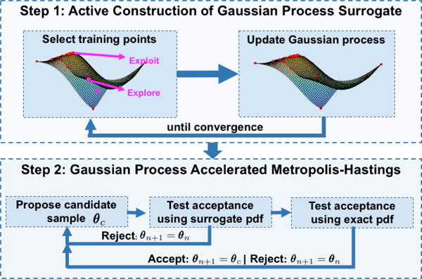
Work-flow diagram of the presented framework.

3.1. Active construction of the GP surrogate

A GP is a random process with an infinite number of random variables, any finite subset of which has a joint Gaussian distribution. It thus provides a distribution over functions $f(\cdot )~\mathcal{G}\mathrm{P}\left(\mu (\cdot ),\kappa \left(\cdot ,\cdot \right)\right)$ that is fully characterized by a mean function μ(·) and a covariance function κ(·, ·) (Rasmussen and Williams, 2006). Over the past few decades, GP has been successfully utilized in many non-linear Bayesian regression tasks. In a typical regression setting, given a set of training input-output pairs Θ = [θ₁, θ₂, …θ_n]^T and G = [g₁, g₂, …g_n]^T, one is interested in making a prediction g_* for any given θ_*. In standard regression with GP, this is achieved by estimating an unobserved latent function that is responsible for generating g from $\mathit{\theta }:g=f\left(\mathit{\theta }\right)+\mathcal{N}\left(0,{\varsigma }^2\right)$. A GP is used to define prior distribution over the latent function $f(\cdot )~\mathcal{G}\mathrm{P}\left(0,\kappa \left(\cdot ,\cdot \right)\right)$. Then, using the properties of Gaussian distribution, the predictive mean μ(θ_*) and variance σ²(θ_*) can be obtained as:

$$\begin{gathered} \mu \left({\mathit{\theta }}_{\ast }\right)={\mathbf{k}}^T{\left(\mathbf{K}+{\varsigma }^2\mathbf{I}\right)}^{-1}\mathbf{G}, \\ {\sigma }^2\left({\mathit{\theta }}_{\ast }\right)=\kappa \left({\mathit{\theta }}_{\ast },{\mathit{\theta }}_{\ast }\right)-{\mathbf{k}}^T{\left(\mathbf{K}+{\varsigma }^2\mathbf{I}\right)}^{-1}\mathbf{k}, \end{gathered}$$ (7)

where k = [κ(θ_*, θ₁), κ(θ_*, θ₂), ⋯ κ(θ_*, θ_n)]^T and K is the positive definite covariance matrix with K_i,_j = κ(θ_i, θ_j).

Because of the analytic properties and the ability to provide probabilistic prediction estimates, recently GP has found widespread use in active learning (Brochu et al., 2010; Kapoor et al., 2007; Krause and Guestrin, 2007; Sun et al., 2015) that is concerned with gathering the most informative training data in cases in which collecting a large number of input-output pairs {Θ, G} is prohibitively expensive (Settles, 2010). In the context of this study, generating training pairs {Θ, G} for building the GP surrogate requires expensive evaluation of the exact posterior pdf at each input θ. Therefore, a method for actively selecting the training points from the parameter space is important. Below, we describe the method that actively selects the training points to obtain an approximation of the posterior pdf model that has higher accuracy in the regions of high posterior pdf.

A GP fitted to the log-posterior pdf is typically better than a GP fitted to the posterior pdf because, in general, the former has longer length scales and lower dynamic range than the latter. Therefore, we fit a GP model for the log of the un-normalized posterior pdf obtained by replacing π(Y|θ) in Eq. (5) with Eq. (6) as given below:

$$g\left(\mathit{\theta }\right)=-\frac{1}{2{\sigma }_e^2}{\Vert \mathbf{Y}-M\left(\mathit{\theta }\right)\Vert }^2+\log \left(\pi \left(\mathit{\theta }\right)\right).$$ (8)

We first define a GP prior over the unknown function (8). Through the covariance function of a GP, assumptions about properties of the function being modeled such as its smoothness and periodicity can be specified. Here, we take an anisotropic Mátern 5/2 co-variance function (Rasmussen and Williams, 2006) that enforces an assumption of twice differentiable function:

$$\kappa \left({\mathit{\theta }}_i,{\mathit{\theta }}_j\right)={\alpha }^2\exp \left(-\sqrt{5}d\left({\mathit{\theta }}_i,{\mathit{\theta }}_j\right)\right)\left(1+\sqrt{5}d\left({\mathit{\theta }}_i,{\mathit{\theta }}_j\right)+5/3d^2\left({\mathit{\theta }}_i,{\mathit{\theta }}_j\right)\right),$$ (9)

where d²(θ_i, θ_j) = (θ_i − θ_j)^TΛ(θ_i − θ_j), Λ is a diagonal matrix with the square of the characteristics length scales along each dimension of θ as the diagonal elements, and α² is the co-variance amplitude. Because no prior knowledge about the posterior pdf is available, here for simplicity we take a zero mean function, which is a commonly and effectively used mean function in GP modeling (Rasmussen and Williams, 2006). The active construction of GP consists of an iteration of two major steps: 1) find a point in the sample space that improves the approximation of Eq. (8), especially in the regions of high posterior pdf, and 2) update the GP at this point.

1. Find optimal training points in the parameter space to update the GP

Here, we assume that the optimal training points are those that will: 1) allow the GP to globally approximate the Eq. (8) well, and 2) identify the regions of high posterior probability. For the former, points are chosen where the predictive uncertainty σ(θ) of current GP is high (to facilitate exploration of uncertain space). For the latter, points are chosen where the predictive mean μ(θ) of the current GP is high (to exploit the current knowledge about the space of high posterior probability). This is done by finding the point that maximizes the upper confidence bound of the GP (Srinivas et al., 2012):

$${\mathit{\theta }}_{n+1}=\underset{\mathit{\theta }}{\arg max}\left\{\mu \left(\mathit{\theta }\right)+{\beta }^{1/2}\sigma \left(\mathit{\theta }\right)\right\}.$$ (10)

The parameter β = 2 log(π²n²/6η), η ∈ (0, 1) balances between exploitation and exploration of the parameter space (Brochu et al., 2010; Srinivas et al., 2012). Eq. (10) is optimized using a bound constrained derivative-free optimization method known as Bound Optimization BY Quadratic Approximation (BOBYQA) (Powell, 2009). The predictive mean and uncertainty in Eq. (10) are evaluated using Eq. (7).

2. Updating the GP surrogate at selected training points

Once a new training point is obtained, Eq. (8) is evaluated at this point and the GP is updated at the newly obtained {θ_n+1, g_n+1} pair. This GP captures the updated belief over Eq. (8) after having observed the new training point.

$$\left[\begin{array}{l}\mathbf{G}\hfill \\ g_{n+1}\hfill \end{array}\right]~\mathcal{N}\left(0,\left[\begin{array}{cc}\mathbf{K}+{\varsigma }^2\mathbf{I}& \mathbf{k}\\ {\mathbf{k}}^{\mathbf{T}}& \kappa \left({\mathit{\theta }}_{n+1},{\mathit{\theta }}_{n+1}\right)\end{array}\right]\right).$$ (11)

where k = [κ(θ_n+1, θ₁), κ(θ_n+1, θ₂), ⋯ κ(θ_n+1,θ_n)]^T, K is the covariance matrix, and ς = 0.001 is a small noise term that is added for numerical stability. After every several updates of the GP, we optimize the hyperparameters (length scales Λ and covariance amplitude α) by maximizing the marginal likelihood log p(g_1:n+1|θ_1:n+1, α, Λ).

These two steps iterate until the training point selected by optimizing the upper confidence bound (10) changes little over a few iterations (≤ 0.005, 15 iterations). The hyperparameters length scales Λ and covariance amplitude α are once again optimized by maximizing the marginal likelihood log p(g_1:n+1|θ_1:n+1, α, Λ). Fig. 2 gives examples of the training points selected during the GP construction, which reveals that these points are spread in the sample space but are more concentrated in the regions of high posterior probability. We take the predictive mean function of the resulting GP as the surrogate of Eq. (8). In this way, we can obtain a GP-based surrogate of the exact posterior pdf π(θ|Y), denoted by π*(θ|Y) for the remainder of this paper, that is cheap to evaluate and is most accurate in regions of high posterior probability.

Figure 2.

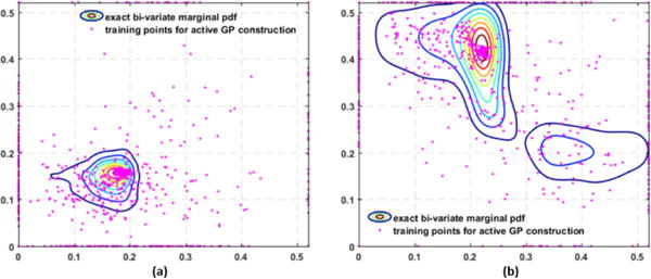
Examples of exact bivariate marginal pdfs superimposed with the training points collected during GP construction, which are spread in the parameter space but are most concentrated in regions of high probability density.

3.2. Gaussian process surrogate accelerated Metropolis-Hastings

MH is the most widely used MCMC method. It begins from an arbitrary sample θ_n and generates a Markov chain of samples that come from an invariant distribution. In specific, at each step in the MH algorithm, a candidate sample θ_c is proposed using a proposal distribution q(θ_c|θ_n). This candidate is accepted with a probability given by:

$${\rho }_{mh}\left({\mathit{\theta }}_n,{\mathit{\theta }}_c\right)=min\left(1,\frac{q\left({\mathit{\theta }}_n|{\mathit{\theta }}_c\right)\pi \left({\mathit{\theta }}_c|\mathbf{Y}\right)}{q\left({\mathit{\theta }}_c|{\mathit{\theta }}_n\right)\pi \left({\mathit{\theta }}_n|\mathbf{Y}\right)}\right).$$ (12)

if accepted, θ_n+1 = θ_c. If rejected, θ_n+1 = θ_n. This is repeated until the samples converge to the target distribution.

The success of the MH largely relies on the choice of the proposal distribution. If the proposal distribution is much narrower than the target distribution, the MH will spend too much time exploring the sampling space, resulting in bad mixing. Conversely, if the proposal distribution is much wider than the target distribution, the MH will make wide jumps in the sampling space, resulting in a large number of rejections. Ideally, a proposal distribution similar to the target distribution is desired for a higher acceptance rate with a good mixing. However, to obtain such a proposal distribution is notoriously difficult and a Gaussian distribution is the most commonly used proposal distribution in practice. Meanwhile, some previous works have proposed the modification of this generic proposal distribution using various approximate target distributions (Christen and Fox, 2005; Efendiev et al., 2006). Below, we describe how a GP surrogate of the posterior pdf is utilized to modify the Gaussian proposal distribution in MH to accelerate sampling with good mixing and a higher acceptance rate.

Specifically, we present a two-step test of acceptance. In the first step, a candidate θ_c1 proposed by a standard Gaussian proposal distribution q(θ_c1|θ_n) is tested for acceptance by the GP surrogate of the posterior pdf π*(θ|Y) with acceptance probability given by:

$${\rho }_1\left({\mathit{\theta }}_n,{\mathit{\theta }}_{c1}\right)=min\left(1,\frac{q\left({\mathit{\theta }}_n|{\mathit{\theta }}_{c1}\right){\pi }^{\ast }\left({\mathit{\theta }}_{c1}|\mathbf{Y}\right)}{q\left({\mathit{\theta }}_{c1}|{\mathit{\theta }}_n\right){\pi }^{\ast }\left({\mathit{\theta }}_n|\mathbf{Y}\right)}\right).$$ (13)

The candidate for the second test of acceptance is determined by the outcome of the previous step, i.e, θ_c = θ_c1 if accepted and θ_c = θ_n if rejected. In other words, the candidates for the second step are effectively generated from the transition probability in the first step, which defines the effective proposal distribution:

$$q^{\ast }\left({\mathit{\theta }}_c|{\mathit{\theta }}_n\right)={\rho }_1\left({\mathit{\theta }}_n,{\mathit{\theta }}_c\right)q\left({\mathit{\theta }}_c|{\mathit{\theta }}_n\right)+r\left({\mathit{\theta }}_n\right){\delta }_{{\mathit{\theta }}_n}\left({\mathit{\theta }}_c\right),$$ (14)

where r(θ_n) = 1 − ∫ ρ₁(θ_n, θ_c)q(θ_c|θ_n)dθ_c is the probability that the chain remains at θ_n and ${\delta }_{{\mathit{\theta }}_n}(\cdot )$ denotes the Dirac mass at θ_n. Using this modified proposal distribution, the proposed candidate sample is accepted by the exact posterior pdf with a probability given by:

$${\rho }_2\left({\mathit{\theta }}_n,{\mathit{\theta }}_c\right)=min\left(1,\frac{q^{\ast }\left({\mathit{\theta }}_n|{\mathit{\theta }}_c\right)\pi \left({\mathit{\theta }}_c|\mathbf{Y}\right)}{q^{\ast }\left({\mathit{\theta }}_c|{\mathit{\theta }}_n\right)\pi \left({\mathit{\theta }}_n|\mathbf{Y}\right)}\right).$$ (15)

Depending on whether the candidate was accepted or rejected in the first step, the acceptance rate in Eq. (15) can be calculated. When a candidate is accepted in the first step, i.e., θ_c = θ_c1, we obtain q*(θ_c|θ_n) = ρ₁(θ_n, θ_c)q(θ_c|θ_n), which can be further simplified using Eq. (13) as follows:

$$\begin{gathered} q^{\ast }\left({\mathit{\theta }}_c|{\mathit{\theta }}_n\right)=min\left(q\left({\mathit{\theta }}_c|{\mathit{\theta }}_n\right){\pi }^{\ast }\left({\mathit{\theta }}_n|\mathbf{Y}\right),q\left({\mathit{\theta }}_n|{\mathit{\theta }}_c\right){\pi }^{\ast }\left({\mathit{\theta }}_c|\mathbf{Y}\right)\right)\frac{1}{{\pi }^{\ast }\left({\mathit{\theta }}_n|\mathbf{Y}\right)} \\ =min\left(\frac{q\left({\mathit{\theta }}_c|{\mathit{\theta }}_n\right){\pi }^{\ast }\left({\mathit{\theta }}_n|\mathbf{Y}\right)}{q\left({\mathit{\theta }}_n|{\mathit{\theta }}_c\right){\pi }^{\ast }\left({\mathit{\theta }}_c|\mathbf{Y}\right)},1\right)q\left({\mathit{\theta }}_n|{\mathit{\theta }}_c\right)\frac{{\pi }^{\ast }\left({\mathit{\theta }}_c|\mathbf{Y}\right)}{{\pi }^{\ast }\left({\mathit{\theta }}_n|\mathbf{Y}\right)} \\ ={\rho }_1\left({\mathit{\theta }}_c,{\mathit{\theta }}_n\right)q\left({\mathit{\theta }}_n|{\mathit{\theta }}_c\right)\frac{{\pi }^{\ast }\left({\mathit{\theta }}_c|\mathbf{Y}\right)}{{\pi }^{\ast }\left({\mathit{\theta }}_n|\mathbf{Y}\right)} \\ =q^{\ast }\left({\mathit{\theta }}_n|{\mathit{\theta }}_c\right)\frac{{\pi }^{\ast }\left({\mathit{\theta }}_c|\mathbf{Y}\right)}{{\pi }^{\ast }\left({\mathit{\theta }}_n|\mathbf{Y}\right)}. \end{gathered}$$ (16)

Substituting Eq. (16) into Eq. (15), the acceptance probability in the second step can be simplified to:

$${\rho }_2\left({\mathit{\theta }}_n,{\mathit{\theta }}_c\right)=min\left(1,\frac{\pi \left({\mathit{\theta }}_c|\mathbf{Y}\right){\pi }^{\ast }\left({\mathit{\theta }}_n|\mathbf{Y}\right)}{\pi \left({\mathit{\theta }}_n|\mathbf{Y}\right){\pi }^{\ast }\left({\mathit{\theta }}_c|\mathbf{Y}\right)}\right).$$ (17)

When a candidate is rejected in the first step, then θ_c = θ_n and ρ₂(θ_n, θ_c) = 1. In other words, samples that are rejected in the first step do not need to be evaluated by the exact posterior pdf. This improves the proposal distribution for the MH method and reduces the need for evaluating the expensive posterior pdf at candidates that are highly unlikely to be accepted.

Convergence of the GP-accelerated MH sampling

The convergence of the MH with modified proposal distribution follows the same line as that of the standard MH (Andrieu et al., 2003; Christen and Fox, 2005; Efendiev et al., 2006; Gilks et al., 1995). Given any initial sample, the Markov chain generated by the MH converges to an invariant distribution if the transition probability meets the following properties: 1) irreducibility, and 2) aperiodicity. A sufficient, but not necessary, condition to ensure convergence to an invariant distribution is reversibility (detailed balance). The presented GP-accelerated MH satisfies these criteria as follows:

• 1)
  Reversibility: Similar to the standard MH, through the inclusion of the acceptance rate, the transition probability is designed to meet the criteria of detailed balance by construction. Specifically, the detailed balance condition is given by:

  $$\pi \left({\mathit{\theta }}_n|\mathbf{Y}\right)T\left({\mathit{\theta }}_c|{\mathit{\theta }}_n\right)=\pi \left({\mathit{\theta }}_c|\mathbf{Y}\right)T\left({\mathit{\theta }}_n|{\mathit{\theta }}_c\right).$$ (18)

  where T denotes the transition probability of the presented GP-accelerated MH method that is defined by:

  $$T\left({\mathit{\theta }}_c|{\mathit{\theta }}_n\right)={\rho }_2\left({\mathit{\theta }}_n,{\mathit{\theta }}_c\right)q^{\ast }\left({\mathit{\theta }}_c|{\mathit{\theta }}_n\right)+\left(1-{\displaystyle \int {\rho }_2\left({\mathit{\theta }}_n,{\mathit{\theta }}_c\right)q^{\ast }\left({\mathit{\theta }}_c|{\mathit{\theta }}_n\right)d{\mathit{\theta }}_c}\right){\delta }_{{\mathit{\theta }}_n}\left({\mathit{\theta }}_c\right).$$ (19)

Proof

When θ_c = θ_n, Eq. (18) is automatically satisfied. When θ_c ≠ θ_n, Eq. (18) can be simplified using Eq. (19) and Eq. (15) as:

$$\begin{gathered} \pi \left({\mathit{\theta }}_n|\mathbf{Y}\right)T\left({\mathit{\theta }}_c|{\mathit{\theta }}_n\right)=\pi \left({\mathit{\theta }}_n|\mathbf{Y}\right){\rho }_2\left({\mathit{\theta }}_n,{\mathit{\theta }}_c\right)q^{\ast }\left({\mathit{\theta }}_n|{\mathit{\theta }}_c\right) \\ =min\left(q^{\ast }\left({\mathit{\theta }}_c|{\mathit{\theta }}_n\right)\pi \left({\mathit{\theta }}_n|\mathbf{Y}\right),q^{\ast }\left({\mathit{\theta }}_n|{\mathit{\theta }}_c\right)\pi \left({\mathit{\theta }}_c|\mathbf{Y}\right)\right) \\ =\pi \left({\mathit{\theta }}_c|\mathbf{Y}\right)min\left(1,\frac{q^{\ast }\left({\mathit{\theta }}_c|{\mathit{\theta }}_n\right)\pi \left({\mathit{\theta }}_n|\mathbf{Y}\right)}{q^{\ast }\left({\mathit{\theta }}_n|{\mathit{\theta }}_c\right)\pi \left({\mathit{\theta }}_c|\mathbf{Y}\right)}\right)q^{\ast }\left({\mathit{\theta }}_n|{\mathit{\theta }}_c\right) \\ =\pi \left({\mathit{\theta }}_c|\mathbf{Y}\right)T\left({\mathit{\theta }}_n|{\mathit{\theta }}_c\right). \end{gathered}$$ (20)

□

• 2)Aperiodicity: Because the acceptance criteria in the presented method always allow for rejection of the samples as in the standard MH, the presented GP-accelerated MH is also aperiodic.
• 3)Irreducibility: If π(θ_c|Y) > 0, ∀θ_c ∈ Ω implies π*(θ_c|Y) > 0, ∀θ_c ∈ Ω, where Ω is the support of the exact posterior pdf π(θ_c|Y), then the Markov chain generated by the presented method is π-irreducible.

Proof

To ensure the condition of irreducibility in the standard MH, the proposal distribution is chosen to satisfy q(θ_c|θ_n) > 0, ∀θ_c, θ_n ∈ Ω. As a result, the transition probability in the standard MH, T_mh(Ω|θ_n) > 0, ∀θ_n ∈ Ω. Using the condition that the GP surrogate of the posterior distribution π*(θ_c|Y) > 0, ∀θ_c ∈ Ω, we can obtain similar results for the transition probability in the first step (alternatively the effective proposal distribution) of the presented method, i.e., q*(θ_c|θ_n) > 0, ∀θ_c, θ_n ∈ Ω. Without the loss of generality, assuming that θ_c ≠ θ_n, we obtain q*(θ_c|θ_n) = ρ₁(θ_n, θ_c)q(θ_c|θ_n) > 0, ∀θ_c, θ_n ∈ Ω from Eq. (14). This implies that ρ₂(θ_n, θ_c)q*(θ_c|θ_n) > 0, ∀θ_c, θ_n ∈ Ω. Therefore, the effective transition probability Eq. (19) of the presented method T(θ_c|θ_n) > 0, ∀θ_c, θ_n ∈ Ω. Hence, under the given condition that π*(θ_c|Y) > 0, ∀θ_c ∈ Ω, the presented method is π-irreducible. Here, the GP surrogate of the posterior distribution π*(θ_c|Y) is an exponential function. Therefore, π*(θ_c|Y) > 0, ∀θ_c ∈ ℝ^d □

In practice, while the theoretical convergence is guaranteed, an inaccurate surrogate model could lead to a biased sampling with a low acceptance rate in the presented method.

4. Evaluation on synthetic data

In experiments with synthetic data, we first evaluate the accuracy and efficiency of the presented method (GP-accelerated MH) against: 1) the baseline of directly sampling the exact posterior pdf using the standard MH (direct MH), and 2) the previously reported approach of directly sampling the surrogate posterior pdf using the standard MH (MH on GP) (Schiavazzi et al., 2016). We then analyze and interpret the obtained posterior pdfs in relation to different factors contributing to parameter uncertainty, primarily under the setting of parameter estimation using two different low-dimensional representations of the spatial parameter space as described in Section 2.

In total, we consider 14 synthetic cases with seven different settings of infarcts, each of which is estimated on two different low-dimensional representations of the spatial parameter space. To represent healthy and infarcted tissues in each case, the parameter a of the AP model (1) is set to 0.15 and 0.50, respectively. Measurement data for parameter estimation is generated in two steps. First, action potentials on the cardiac mesh are simulated using the AP model (1). Then, 120-lead ECG are generated using the forward model (2) and corrupted with 20 dB Gaussian noise.

All MCMC sampling runs on four parallel MCMC chains of length 20,000 with a common Gaussian proposal distribution and four different initial points. The variance of the Gaussian proposal distribution is tuned by rapidly sampling the GP surrogate pdf until obtaining an acceptance rate of ∼ 0.22, which is documented to enable good mixing and faster convergence in higher dimensional problems (Andrieu et al., 2003; Gilks et al., 1995). The four initial points are obtained by conducting a rapid sampling of the GP surrogate pdf, constructing four clusters of the samples using a Gaussian mixture model, and using the mean of each as the starting points for each chain. After discarding initial burn-in samples and selecting alternate samples to avoid auto-correlation in each chain, the samples from four chains are combined. The convergence of all the MCMC chains is tested using trace plots, Geweke statistics, and Gelman-Rubin statistics (Andrieu et al., 2003; Gilks et al., 1995). To differentiate the infarcted and healthy regions from the estimated tissue properties, we calculate a threshold value that minimizes the intra-region variance on the estimated parameter values (Otsu, 1975).

4.1. Validation of the accuracy and efficiency of the presented method

We first validate the accuracy of the presented method against directly sampling the exact posterior pdf using the standard MH method. Fig. 3 presents four examples of posterior pdfs obtained from different synthetic data cases. As shown, the presented sampling strategy (green curve) closely reproduces the true posterior pdf (red curve) obtained from direct MH.

Figure 3.

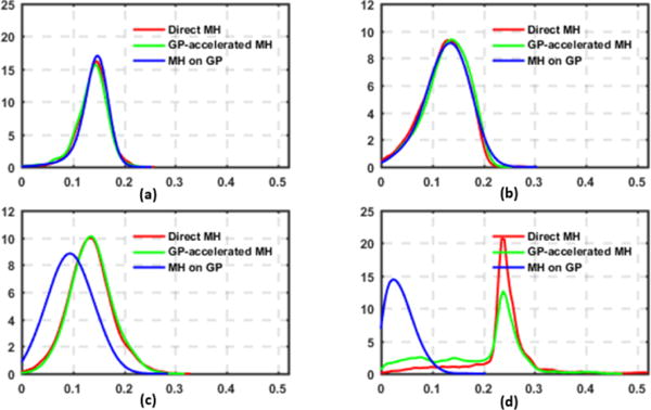
Examples of the exact posterior pdfs (red) vs. those obtained by the presented method (green) and sampling the GP surrogate pdf (blue).

Next, we compare the computational cost of the presented method with that of the direct MH in terms of the number of model evaluations needed and actual computation times. The comparison is based on 14 synthetic cases run on a computer with a Xeon E5 2.20 GHz processor and 128 GB RAM. The presented method reduces the number of model evaluations by an average of 64.47% despite the overhead of constructing the GP surrogate which, as highlighted in the purple bar in Fig. 4 left, is very small compared with the number of model evaluations required for sampling. The computation time is reduced from 41.073±2.028 hours with direct MH to 7.961±2.028 hours with the presented method.

Figure 4.

Comparison of the efficiency between the presented method (GP-accelerated MH) and the standard MH method (Direct MH). Left: computational cost. Right: acceptance rate.

The efficiency of the sampling method is also measured in terms of its acceptance rate. Here, acceptance rate refers to the fraction of the accepted candidates out of all those proposed to the exact posterior pdf. As shown in the right panel of Fig. 4, the presented method improves the acceptance rate from 0.2653 ± 0.0500 of the direct MH to 0.3988 ± 0.0788. This means that the presented method is able to improve the proposal distribution by filtering out a large portion of candidate samples that would eventually be rejected by the exact posterior pdf, thereby avoiding evoking expensive simulation models on these candidates.

4.2. Comparison with directly sampling the GP surrogate

Directly sampling the GP surrogate pdf instead of the exact pdf, as commonly done in existing methods (Schiavazzi et al., 2016), requires significantly less computation because model simulation is not needed. However, the sampling accuracy also becomes critically reliant on the accuracy of the surrogate model. As illustrated in the examples in Figs. 3c and 3d, sampling the GP surrogate (blue curve) produces a distribution that is different from the exact pdf not only in general shape but also in locations of the mode. In comparison, while the accuracy in the GP surrogate affects the efficiency of the presented method, the estimated pdf converges to the exact pdf as obtained by the direct MH. Using the mean, mode, and standard deviation of the exact pdf as the baseline, Table 1 shows that sampling errors of the presented method are significantly lower than those from sampling the surrogate only (paired t-test on 139 estimated parameters, p < 0.001).

Table 1.

Mean absolute errors in the estimated mean, mode, and standard deviation against directly sampling the exact posterior pdf: the presented method (GP-accelerated MH) vs. sampling the GP surrogate pdf only (MH on GP).

Method	Mean	Mode	Standard deviation
GP-accelerated MH	0.012	0.030	0.006
MH on GP	0.039	0.058	0.015

4.3. Analysis of the sampled posterior distributions

Several factors can contribute to the uncertainty in the estimated model parameters, including but not limited to the sparse measurement data, parameter correlation, model over-parameterization, and limited spatial resolution in comparison with the underlying tissue heterogeneity (which we will refer to as “model under-parameterization” for the remainder of the paper). Some of these factors vary with the method used to represent the parameter space. For example, different low-dimensional representations of the parameter space may result in different correlations between each dimension of the parameter, as well as different over- and/or under-parameterization of the model. Therefore, in this section, we consider the presented approach on two types of low-dimensional representations of the parameter space: a uniform division of the cardiac mesh into 10 segments using the AHA standard, and a non-uniform division of the cardiac mesh into 7-15 clusters using a method that aims to adaptively group homogeneous nodes of the cardiac mesh together (Dhamala et al., 2016). Below, we analyze and interpret the estimated posterior pdfs in relation to the aforementioned contributing factors to uncertainty. We elaborate on three examples with a varying degree of “parameter heterogeneity”, a term we use to denote a state in which a dimension of the parameter representation is too low in resolution to reflect the underlying heterogeneity.

In the first example shown in Fig. 5, the infarct in the septum region is better represented by the uniform method than the adaptive method with respect to parameter heterogeneity. Specifically, the uniform method generates three heterogeneous segments that are 37.32% of the heart volume; in comparison, the adaptive method generates four heterogeneous clusters that are 53.09% of the heart volume. In this case, the mode estimated using the uniform method accurately captures the infarct region (Dice coefficient: 0.5896), whereas the adaptive method captures the infarct with false positives at the right ventricle (Dice coefficient: 0.3447). Correspondingly, while the uniform method shows high confidence in the solution obtained in the region of true infarct, the adaptive method shows high uncertainty in the region of true infarct. In addition, it is interesting to note that both low-dimensional representations result in high parameter uncertainty at the right ventricle region and the anterior region adjacent to the region of infarct. This uncertainty, independent of the low-dimensional representation of choice, may indicate difficulty in estimating parameters in this region of the heart due to non-identifiability and limited measurement data.

Figure 5.

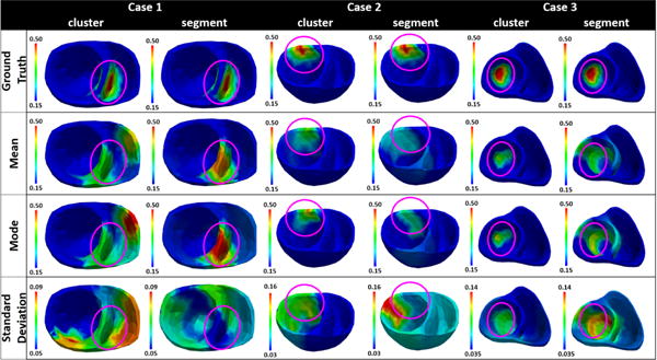
Examples of parameter estimation results when using clusters from the adaptive method vs. segments from the uniform method as low-dimensional representation of the spatial parameter space. Case 1, case 2, and case 3 respectively show an example in which the infarct is represented better by the segments, equally by both segments and clusters, and better by the clusters in terms of parameter heterogeneity.

In the second example that has an infarct in the anterior region as shown in Fig. 5, both the uniform and adaptive methods show similar parameter heterogeneity in representing the infarct. Specifically, with the uniform method, the infarct lies completely within a segment such that only one segment that is 10.42% of the heart volume contains heterogeneous tissue; in comparison, the adaptive method generates three heterogeneous clusters that is 10.16% of the heart volume. As shown, using the uniform method, the estimated mode reveals higher parameter value in the segment that contains the infarct (Dice coefficient: 0.1622) with high confidence. However, the standard deviation plot shows high uncertainty in the estimated parameters throughout the cardiac mesh, possibly to compensate for the fact that the true infarct is much smaller than the segment representing the infarct. In comparison, using the adaptive method, the estimated mode has high parameter value in a narrower region representing the compact infarct with higher accuracy (Dice coefficient: 0.5763). Likewise, high parameter uncertainty is obtained in a more concentrated region that overlaps the heterogeneous clusters. Additionally, similar to the first example, both low-dimensional representations show high uncertainty in the region that is adjacent on the left to the region of true infarct. This indicates difficulty in accurately estimating parameters in those regions, possibly again due to non-identifiability and limited data.

Finally, Fig. 5 case 3 shows an example in which an infarct is better represented by the adaptive method than the uniform method with respect to parameter heterogeneity. Specifically, uniform method generates five segments with heterogeneous tissue, totaling 45.01% of the heart volume; in comparison, the adaptive method also generates five clusters with heterogeneous tissue, but totaling only 30.59% of the heart volume. In this case, the mode obtained using the adaptive method captured the region of infarct with higher accuracy (Dice coefficient: 0.6220) than the mode obtained using the uniform method (Dice coefficient: 0.3269). A closer look at the standard deviation plots reveals that, in general, high uncertainty is obtained in the regions of heterogeneous tissue when using either method. Overall, because a higher proportion of the cardiac mesh is associated with heterogeneous representations when using the uniform method (model under-parameterization), an overall larger region of high parameter uncertainty is obtained with the uniform method compared with the adaptive method.

While the issue of model under-parameterization is more evident with the uniform method as explained above, the issue of model over-parameterization is more evident with the adaptive method. This is because the adaptive method as described in Dhamala et al. (2017a) could result in a large number of small clusters at heterogeneous regions around the infarct. Consequently, parameter values at these regions are associated with a high uncertainty as seen in the standard deviation plots obtained by using the adaptive method in Fig. 5, likely due to the issue of non-identifiability given limited and indirect measurement data. An example case, in which this issue is more pronounced, is shown in Fig. 6. Here, several small clusters (c-e) are formed by the adaptive method at the region of the inferior-lateral infarct and its border. For parameter values at these clusters, the MH sampling has difficulty converging to a distribution with distinct modes, which is reflected as high uncertainty in the resulting parameter values. These examples show that probabilistic parameter estimation can help reveal the issue of identifiability, which cannot be observed when a single point estimate is being sought.

Figure 6.

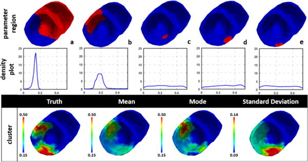
Example of high uncertainty associated with over-parameterization when the adaptive method assigned several small clusters to represent the heterogeneous regions around the infarct (c-e). Top row: clusters represented by one dimension of the parameter space. Middle row: univariate marginal density plot of the estimated parameter. Bottom row: estimated mean, mode and standard deviation of the parameter.

Finally, different low-dimensional representations of the parameter space can also result in different correlations among the parameters in each dimension. In Fig. 7, we show an example with an infarct localized in the septal region, in which the parameter of one of the regions shows both a positive correlation and a negative correlation with parameters in other regions. As shown at the top of Fig. 7c, the parameter in region 7 and region 6 exhibits a negative correlation with a switching behavior (i.e., when the parameter in region 7 is estimated in a healthy range, the parameter in region 6 is estimated in an unhealthy range). At the same time, the parameter in region 7 and region 5 exhibit a positive correlation (i.e., when the parameter in region 7 is estimated in a healthy range, the parameter in region 6 also is estimated in a healthy range; Fig. 7c, bottom). This is reflected as higher parameter uncertainty in all three regions.

Figure 7.

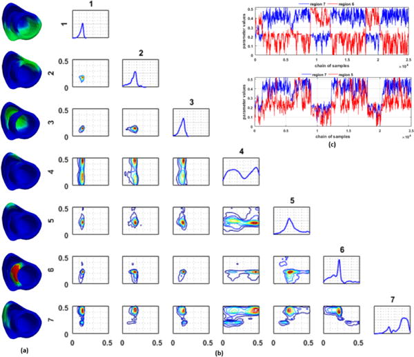
(a) Regions of the heart obtained by the adaptive method. (red: infarct, green: non-infarct/mixed). (b) Estimated univariate and bivariate marginal pdf plots. Numbers on the top and left of pdf plots correspond to regions represented by the pdf plots. (c) Trace plot for parameters of regions 6 and 7 (top) shows a negative correlation with a switching behavior, whereas that of regions 5 and 7 (bottom) shows a positive correlation.

5. Evaluation on a blinded EP model and in-vivo MRI scar

In this section, we study the presented method in quantifying the uncertainty in model parameters for post-infarction human hearts, where validation data for the 3D myocardial infarct is available from in-vivo magnetic resonance imaging. Compared with the infarct settings in synthetic data experiments, these MRI-derived 3D infarcts have the following characteristics that increase the heterogeneity in tissue properties: 1) the presence of both dense scar core and gray zone, 2) the presence of a single or multiple scars with complex spatial distribution and irregular boundaries, and 3) the presence of both transmural and non-transmural scars. The resolution to which such heterogeneity can be captured is largely limited by the method of dimensionality reduction. Because previous work has shown that an adaptive non-uniform low-dimensional representation may be able to better represent tissue heterogeneity (Dhamala et al., 2017a), the experiments below are conducted using only the adaptive low-dimensional representation of the parameter space. Because in-vivo electrical mapping data were unavailable, here measurement data for probabilistic parameter estimation are generated by a high-resolution (average resolution: 350 μm) multi-scale (sub-cellular to organ scale) in-silico ionic electrophysiological model on the MRI-derived patient-specific ventricular models as detailed in Arevalo et al. (2016). Data used for parameter estimation are extracted from 300-400 epicardial sites, temporarily down-sampled to a 5 ms resolution, and corrupted with 20 dB Gaussian noise. Note that although no in-vivo electrical data were available, the experiments are designed to mimic a real-data scenario because: 1) the 3D EP model used to generate the measurement data is known to be capable of generating high-fidelity EP simulation of patient-specific hearts (Arevalo et al., 2016), 2) this model is unknown to the framework of GP-accelerated MH and thus no “inverse crime” is involved, and 3) only a small subset of epicardial data corrupted with noise is used as measurement data.

For clarity, below we analyze the performance of the presented method with respect to two contributing factors to the heterogeneity of the scar: 1) scar transmurality, and 2) gray zone. For ground truth, these regions were determined from the 3D infarcts mapped to the high resolution cardiac mesh from MRI Arevalo et al. (2016).

1) Scar transmurality

In examples case 1, case 2, and case 3 shown in Fig. 8, a portion of the scar is non-transmural. From left to right, the non-transmural portion of the scar lies respectively on the lateral wall, the anterior-septal region, and the anterior-lateral wall of the left ventricle as denoted by a purple circle. In all three cases, the estimated mode misses these regions of non-transmural scar; the estimated mean exhibits higher parameter values deviating from that for healthy tissue, yet the value is not as high as that for scar tissue. In all cases, parameter values in these regions are associated with high uncertainty. This provides a useful confidence measure for the estimated mode, suggesting that these regions do not consist entirely of healthy tissue as reflected by the mode.

Figure 8.

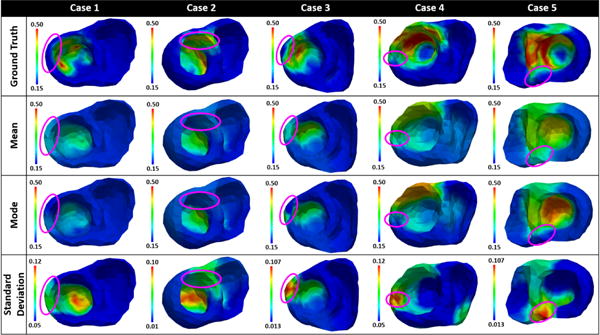
Mean, mode, and standard deviation of posterior pdfs estimated from epicardial potentials simulated by a multi-scale ionic EP model blinded to the presented estimation method. Purple circles denote areas of non-transmural scars (cases 1, 2, and 3) or gray zones (cases 4 and 5).

2) Gray zone

Case 4 and case 5 in Fig. 8 show examples in which a trans-mural dense scar is surrounded by gray zone. In both cases, the mean and mode estimates obtain high parameter values in the region of dense scar and gray zone. The parameter values in the regions of dense scar are higher than those in gray zones. In addition, the mean estimates reveal the gray zone to be wider than the estimates from MRI data, whereas the mode estimates do not. Parameters for these border regions are associated with high uncertainty as shown in the standard deviation plots, reflecting the underlying tissue heterogeneity in these regions and the possible model under-parametrization as a result of the low-dimensional representation of the parameter space.

6. In-vivo evaluation using 120-lead ECG and catheter data

We conduct real-data studies on three patients who underwent catheter ablation of ventricular tachycardia due to prior myocardial infarction (Sapp et al., 2012). The patient-specific heart-torso geometrical models are constructed from axial computerized tomography images. The uncertainty of tissue excitability in the AP model (1) is estimated from 120-lead ECG. Similarly, all experiments are conducted using the adaptive low-dimensional representation of the parameter space (Dhamala et al., 2017a). For validation of the results, we consider the relation between the estimated tissue excitability and the in-vivo epicardial bipolar voltage data obtained from catheter mapping. It should, however, be noted that voltage data can be used only as a reference, not as the gold standard for the measure of tissue excitability. Below we focus our analysis on how the obtained parameter uncertainty is associated with the heterogeneity of the underlying tissue.

Case 1

The voltage data for case 1 (Fig. 9a) shows a dense infarct at inferolateral left ventricle (LV) with a heterogeneous region extending to lateral LV. Adaptive dimensionality reduction as described in Dhamala et al. (2017a) generates eight regions of the heart to be parameterized, five of which are listed in Fig. 10 along with the estimated posterior marginal pdfs for their parameters. As shown, the parameter for the region of infarct core (a) is correctly estimated with high confidence. The parameter for the region of immediate border to the infarct (e) has a mean/mode value that is in between the healthy and infarct core, correctly indicating a border zone, whereas other regions in the infarct border are estimated as either healthy (c-d) or infarcted (b). For all these regions around the heterogeneous infarct border (b-e), uncertainties of the estimation are higher. This produces an estimation with correct posterior mode/mean with high confidence at the infarct core, and high uncertainty at the heterogeneous infarct border.

Figure 9.

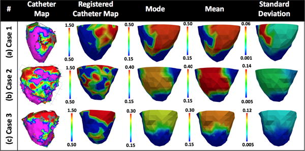
Mean, mode, and standard deviation of the posterior parameter pdfs estimated from 120-lead ECG data.

Figure 10.

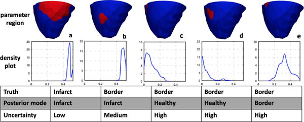
Real-data experiments for case 1 from Fig. 9: regions of the heart to be parameterized and the corresponding marginal probability density plots.

Case 2

The voltage data for case 2 (Fig. 9b) shows a massive yet quite heterogeneous infarct at lateral LV. The adaptive dimensionality reduction method generates 12 regions of the heart to be parameterized, five of which are listed in Fig. 11 along with the estimated marginal pdfs for their parameters. As shown, for remote healthy regions (a-b), their parameters are correctly estimated with high confidence. For heterogeneous border regions close to the infarct (c-d), their parameters are estimated in the healthy range but with lower confidence. For the region that corresponds to the infarct (e), its abnormal parameter is correctly captured but with a high uncertainty – likely reflecting the heterogeneous nature of tissue properties in this region. As summarized in Fig. 9b, while the estimation correctly reveals the region of infarct as in case 1, it is also associated with a higher uncertainty compared with the less heterogeneous infarct in case 1.

Figure 11.

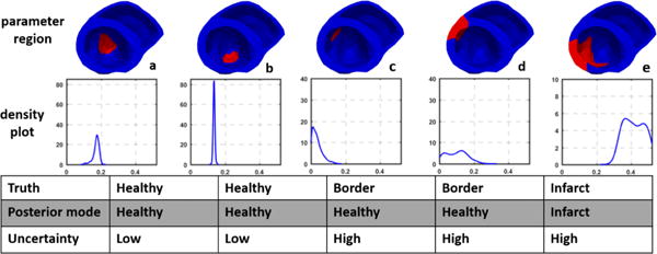
Real-data experiments for case 2 from Fig. 9: regions of the heart to be parameterized and the corresponding marginal probability density plots.

Case 3

The voltage data for case 3 (Fig. 9c) shows low voltage at lateral LV and RV, although it was not certain whether the low voltage on lateral RV was due to the presence of an infarct or fat layer. After dimensionality reduction with the adaptive method, there are seven regions of the heart that remain to be parameterized (Fig. 12a). The infarct region in lateral LV (region 1) is estimated with a distribution that has medium uncertainty and a mode of 0.257. This could indicate the presence of infarcted tissue along with some healthy tissue (heterogeneity). In contrast, the marginal distribution for the healthy apical region (region 2) is estimated with a very narrow uni-modal distribution with a mode of 0.142. Interestingly, several regions in the lateral RV (region 4, 5, and 7) show very high uncertainty with a distribution of the parameter value extending from healthy to infarct range. Overall, results show an estimate of healthy tissue in the apical region with high confidence, an estimate of heterogeneous tissue with infarct at lateral LV with medium confidence (Fig. 9c), and an estimate of the ambiguous region in lateral RV as healthy with high uncertainty.

Figure 12.

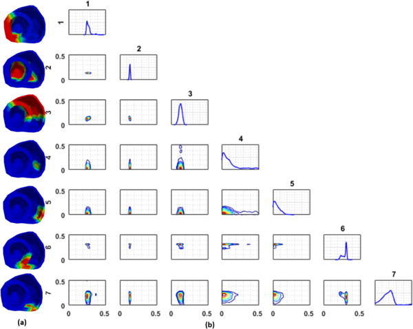
Real-data experiments for case 3 from Fig. 9. (a) Regions of the heart to be parameterized. (b) Univariate and bivariate marginal pdf plots.

7. Discussion

7.1. Quality of the surrogate vs. acceptance rate

To understand how the acceptance rate of the presented GP-accelerated MH method is related to the accuracy of the GP surrogate, we measure the quality of the GP surrogates built in the synthetic data experiments by their Kullback-Leibler (KL) divergence to the exact posterior pdfs. The KL-divergence from the GP surrogate pdf π*(θ|Y) to the exact posterior pdf π(θ|Y) is defined by:

$$D_{KL}\left(\pi \left(\mathit{\theta }|\mathbf{Y}\right)\Vert {\pi }^{\ast }\left(\mathit{\theta }|\mathbf{Y}\right)\right)={\displaystyle {\int }_{-\mathrm{\infty }}^{\mathrm{\infty }}\pi \left(\mathit{\theta }|\mathbf{Y}\right)\log \left(\frac{\pi \left(\mathit{\theta }|\mathbf{Y}\right)}{{\pi }^{\ast }\left(\mathit{\theta }|\mathbf{Y}\right)}\right)}d\mathit{\theta }.$$ (21)

Because above KL divergence cannot be obtained analytically, we estimate it using Monte Carlo simulation (Hershey and Olsen, 2007) as follows:

$$D_{KL}\left(\pi \left(\mathit{\theta }|\mathbf{Y}\right)\Vert {\pi }^{\ast }\left(\mathit{\theta }|\mathbf{Y}\right)\right)=\frac{1}{N}{\displaystyle \sum _{i=1}^N\log \left(\frac{\pi \left({\mathit{\theta }}_i|\mathbf{Y}\right)}{{\pi }^{\ast }\left({\mathit{\theta }}_i|\mathbf{Y}\right)}\right)},$$ (22)

where θ_i are N random samples of π(θ|Y) obtained from direct MH method. As shown in Fig. 13, in most cases, the KL divergence of the surrogate pdf is low, indicating a high accuracy of the surrogate pdf. However, some surrogate pdfs had a high KL divergence from the exact pdf, indicating limited accuracy which is most likely related to the increased complexity in the shape of the un-normalized log exact posterior pdf. As expected, a negative correlation between the quality of the GP surrogate and the acceptance rate of the GP-accelerated MH method (correlation coefficient = −0.777) can be observed in Fig. 13. In other words, a more accurate GP surrogate will result in a higher efficiency of the presented sampling method, whereas a less accurate GP surrogate would be less effective in accelerating the MH sampling. However, a more accurate GP surrogate would also be more expensive to construct, whereas a less accurate one would be faster to construct. How to balance between these two steps, as well as how to construct an accurate surrogate without evoking a large number of model evaluations, are to be investigated in future works.

Figure 13.

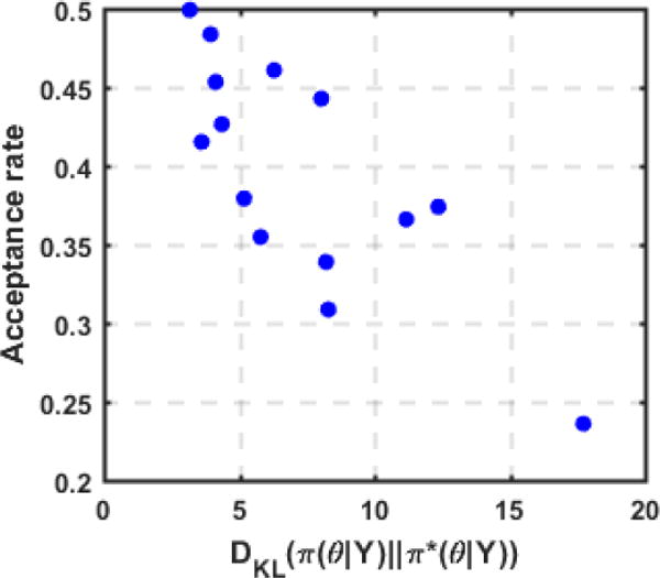
Acceptance rate of the GP-accelerated MH method decreases as the KL-divergence from the GP surrogate to the exact posterior pdf increases. Data is taken from the sampled distributions in synthetic data experiments.

7.2. Related works

Related works on uncertainty quantification in personalized models can be broadly categorized into two types: 1) forward uncertainty quantification, and 2) inverse uncertainty quantification. Forward uncertainty quantification focuses on the uncertainty in model output as a result of variations in different model parameters. To overcome the challenge of repeatedly evaluating the expensive simulation model, methods such as generalized polynomial chaos or stochastic collocation are commonly used. In the domain of electrocardiography, this includes examples such as the study of sensitivity of model output to conductivity parameters (Geneser et al., 2008), the study of sensitivity of measured ECG signals on heart motion (Swenson et al., 2011), and the study of sensitivity of ECG signal components as a result of variations in sub-endocardial ischemia (Johnston et al., 2017). These works are fundamentally different from the presented work that focuses on the inverse uncertainty quantification.

The inverse uncertainty quantification focuses on the uncertainty within the model (such as the estimated model parameters) as a result of different uncertain factors involved in the personalization of the model. Among existing works, the approach presented in Lê et al. (2016), although applied to a brain tumor growth model, is most common in its spirit with the presented framework. Specifically, the work presented in Lê et al. (2016) also utilizes a two stage sampling method (GPHMC) in which first a GP surrogate of the unnormalized negative log posterior pdf is learned with HMC and then its gradient is uti-lized in HMC for efficient sampling. To compare the presented method and the GPHMC method, we conducted experiments on six synthetic cases. Implementation of the GPHMC method as detailed in Lê et al. (2016) is utilized. We take 50 initialization points and 3000 exploratory points during the construction of the GP surrogate. The comparison is presented with respect to the two major elements of these methods: 1) GP surrogate construction, and 2) posterior pdf sampling. For the constructed GP surrogates, their mean KL divergences to the exact posterior pdf are respectively 6.58 and 38.57 for the presented method and the GPHMC method. This gain in accuracy by the presented method could be because of the utilization of a Mátern 5/2 kernel in GP, and an active scheme with a derivative free deterministic optimization to select training points. An increase in the number of training points in the GPHMC method may increase the accuracy of the GP surrogate. For the posterior pdf sampling, surprisingly we observed an acceptance rate of ≤ 0.1 with GPHMC although the accuracy of the GP surrogate was comparable between the two methods. We speculate that given the non-smooth and complex shape of the negative log posterior pdf and its first derivative in this study, a GP – especially one with a squared exponential kernel that assumes an infinitely differentiable prior over the negative log posterior pdf – could not accurately approximate its local derivatives. This inaccuracy in the approximated local derivatives may then lead to poor candidate samples proposed by the HMC, resulting in low acceptance rate. In contrast, because the presented method only depends on the approximate global shape of the log posterior pdf without utilizing its derivative information in the sampling, a smoother approximation such as a GP with Mátern 5/2 kernel could increase the acceptance rate.

The selection of points for the construction of a GP surrogate shares common intuition with active learning (Kapoor et al., 2007), Bayesian optimization (Brochu et al., 2010), and multi-armed bandits problems (Srinivas et al., 2012) in which based on a history of actions and rewards a decision needs to be made on the next best point to query from the solution space. More recently, there has been an interest in utilizing these methods to approximate intractable pdfs (Kandasamy et al., 2015). In contrast to these works that focus on obtaining a surrogate model that can directly replace the exact pdf, the presented framework focuses on utilizing this surrogate to accelerate the sampling without a compromise in accuracy.

8. Conclusion

In this paper, we present a novel framework to efficiently yet accurately sample the posterior distribution of parameters in patient-specific cardiac elec-trophysiological models. This is achieved by first an active construction of an efficient GP surrogate of the posterior pdf, followed by the use of this surrogate to improve the proposal distribution of the standard MH. The presented method is evaluated on both synthetic and real data experiments. Our future work will investigate methods to further improve the accuracy of the surrogate model, without requiring a large number of model evaluations. We will also investigate an adaptive GP-accelerated MH method that will continuously update the surrogate GP with accepted samples during sampling.

Appendix A. Spatially-adaptive multi-scale parameter estimation

The spatially-adaptive multi-scale parameter estimation framework generates a non-uniform representation of the parameter space consisting of higher resolution in the heterogeneous tissue regions and low resolution is the homogeneous tissue regions (Dhamala et al., 2016). To achieve this, it consists of three major components: 1) a multi-scale hierarchical representation of the cardiac mesh, 2) a coarse-to-fine optimization, and 3) a criterion for adaptive spatial resolution adjustment. First, a coarse-to-fine hierarchical representation of the cardiac mesh is generated using a bottom-up hierarchical clustering on the nodes of the cardiac mesh. The average of the pairwise Euclidean distances between each node in two clusters is taken as the similarity measure during clustering. Next, beginning from the coarsest scale of the multi-scale hierarchy, optimization and spatial resolution adjustment are carried out alternatively along the multi-scale hierarchy. During this, the optimization step is used to estimate the optimal parameters at the present resolution and the spatial resolution adjustment step is used to determine the next appropriate resolution. This is done until further resolution refinement does not improve the optimization result. In specific, in the optimization step, an objective function consisting of the negative correlation coefficient and sum of the squared error between the measurement ECG signal and the simulated ECG signal with parameters at the current resolution is optimized. In the adaptive spatial resolution adjustment step, clusters at the present resolution are identified to be refined or coarsened by calculating the gain as a result of their refinement in the objective function value as follows. For each pair of sibling clusters that were refined from a common parent cluster, the gain is computed as the change in the objective function value with current optimal parameter value versus replacing the values of the sibling clusters with the value of their parent cluster. For clusters that do not have a sibling due to previous coarsening, the gain equals the change in the objective function value due to the change in its value during the coarsening and after the optimization. The cluster with a maximum gain is further refined, whereas clusters with no gain are coarsened. This refinement and coarsening is carried out along the multi-scale hierarchy. We show an example of the final parameter regions obtained by this method and the 10 regions obtained by the AHA model in Fig. A.14.

Figure A.14.

An example of division of heart into regions used in this paper: (a) ground truth infarct setting, (b) regions obtained by the spatially adaptive method shows higher resolution along infarcted region, and (c) 10 fixed regions obtained from the AHA model.

References

- Aliev RR, Panfilov AV. A simple two-variable model of cardiac excitation. Chaos, Solitons & Fractals. 1996;7:293–301. [Google Scholar]
- Andrieu C, De Freitas N, Doucet A, Jordan MI. An introduction to mcmc for machine learning. Machine learning. 2003;50:5–43. [Google Scholar]
- Arevalo HJ, Vadakkumpadan F, Guallar E, Jebb A, Malamas P, Wu KC, Trayanova NA. Arrhythmia risk stratification of patients after myocardial infarction using personalized heart models. Nature communications. 2016;7 doi: 10.1038/ncomms11437. [DOI] [PMC free article] [PubMed] [Google Scholar]
- Brochu E, Cora VM, De Freitas N. A tutorial on bayesian optimization of expensive cost functions, with application to active user modeling and hierarchical reinforcement learning. arXiv preprint arXiv. 2010;1012:2599. [Google Scholar]
- Cerqueira MD, Weissman NJ, Dilsizian V, Jacobs AK, Kaul S, Laskey WK, Pennell DJ, Rumberger JA, Ryan T, Verani MS, et al. Standardized myocardial segmentation and nomenclature for tomographic imaging of the heart a statement for healthcare professionals from the cardiac imaging committee of the council on clinical cardiology of the american heart association. Circulation. 2002;105:539–542. doi: 10.1161/hc0402.102975. [DOI] [PubMed] [Google Scholar]
- Chinchapatnam P, Rhode KS, Ginks M, Mansi T, Peyrat JM, Lam-biase P, Rinaldi CA, Razavi R, Arridge S, Sermesant M. Estimation of volumetric myocardial apparent conductivity from endocardial electro-anatomical mapping. Engineering in Medicine and Biology Society, 2009. 2009:2907–2910. doi: 10.1109/IEMBS.2009.5334441. EMBC 2009. Annual International Conference of the IEEE, IEEE. [DOI] [PubMed] [Google Scholar]
- Chinchapatnam P, Rhode KS, Ginks M, Rinaldi CA, Lambiase P, Razavi R, Arridge S, Sermesant M. Model-based imaging of cardiac apparent conductivity and local conduction velocity for diagnosis and planning of therapy. Medical Imaging, IEEE Transactions. 2008;27:1631–1642. doi: 10.1109/TMI.2008.2004644. [DOI] [PubMed] [Google Scholar]
- Christen JA, Fox C. Markov chain monte carlo using an approximation. Journal of Computational and Graphical statistics. 2005;14:795–810. [Google Scholar]
- Clayton R, Bernus O, Cherry E, Dierckx H, Fenton F, Mirabella L, Panfilov A, Sachse FB, Seemann G, Zhang H. Models of cardiac tissue electrophysiology: progress, challenges and open questions. Progress in biophysics and molecular biology. 2011;104:22–48. doi: 10.1016/j.pbiomolbio.2010.05.008. [DOI] [PubMed] [Google Scholar]
- Dhamala J, Arevalo H, Sapp J, Horacek M, Wu K, Trayanova N, Wang L. Spatially-adaptive multi-scale optimization for local parameter estimation in cardiac electrophysiology. IEEE Transactions on Medical Imaging. 2017a doi: 10.1109/TMI.2017.2697820. [DOI] [PMC free article] [PubMed] [Google Scholar]
- Dhamala J, Sapp JL, Horacek M, Wang L. International Conference on Medical Image Computing and Computer-Assisted Intervention. Springer; 2016. Spatially-adaptive multi-scale optimization for local parameter estimation: application in cardiac electrophysiological models; pp. 282–290. [Google Scholar]
- Dhamala J, Sapp JL, Horacek M, Wang L. International Conference on Information Processing in Medical Imaging. Springer; 2017b. Quantifying the uncertainty in model parameters using gaussian process-based markov chain monte carlo: An application to cardiac electrophysiological models; pp. 223–235. [Google Scholar]
- Efendiev Y, Hou T, Luo W. Preconditioning markov chain monte carlo simulations using coarse-scale models. SIAM Journal on Scientific Computing. 2006;28:776–803. [Google Scholar]
- Geneser SE, Kirby RM, MacLeod RS. Application of stochastic finite element methods to study the sensitivity of ecg forward modeling to organ conductivity. IEEE Transactions on Biomedical Engineering. 2008;55:31–40. doi: 10.1109/TBME.2007.900563. [DOI] [PubMed] [Google Scholar]
- Giffard-Roisin S, Jackson T, Fovargue L, Lee J, Delingette H, Razavi R, Ayache N, Sermesant M. Noninvasive personalization of a cardiac electrophysiology model from body surface potential mapping. IEEE Transactions on Biomedical Engineering. 2017;64:2206–2218. doi: 10.1109/TBME.2016.2629849. [DOI] [PubMed] [Google Scholar]
- Gilks WR, Richardson S, Spiegelhalter D. Markov chain Monte Carlo in practice. CRC press; 1995. [Google Scholar]
- Hershey JR, Olsen PA. Approximating the kullback leibler divergence between gaussian mixture models. Acoustics, Speech and Signal Processing, 2007. 2007:IV–317. ICASSP 2007. IEEE International Conference on, IEEE. [Google Scholar]
- Johnston BM, Coveney S, Chang ET, Johnston PR, Clayton RH. Quantifying the effect of uncertainty in input parameters in a simplified bido-main model of partial thickness ischaemia. Medical & biological engineering & computing. 2017:1–20. doi: 10.1007/s11517-017-1714-y. [DOI] [PMC free article] [PubMed] [Google Scholar]
- Kandasamy K, Schneider J, Póczos B. Bayesian active learning for posterior estimation. Twenty-Fourth International Joint Conference on Artificial Intelligence 2015 [Google Scholar]
- Kapoor A, Grauman K, Urtasun R, Darrell T. Active learning with gaussian processes for object categorization. Computer Vision, 2007. 2007:1–8. ICCV 2007. IEEE 11th International Conference on, IEEE. [Google Scholar]
- Konukoglu E, Relan J, Cilingir U, Menze BH, Chinchapatnam P, Ja-didi A, Cochet H, Hocini M, Delingette H, Ja¨ıs P, et al. Efficient probabilistic model personalization integrating uncertainty on data and parameters: Application to eikonal-diffusion models in cardiac electrophysiology. Progress in biophysics and molecular biology. 2011;107:134–146. doi: 10.1016/j.pbiomolbio.2011.07.002. [DOI] [PubMed] [Google Scholar]
- Krause A, Guestrin C. Nonmyopic active learning of gaussian processes: an exploration-exploitation approach. Proceedings of the 24th international conference on Machine learning, ACM. 2007:449–456. [Google Scholar]
- Lê M, Delingette H, Kalpathy-Cramer J, Gerstner ER, Batchelor T, Unkelbach J, Ayache N. Mri based bayesian personalization of a tumor growth model. IEEE transactions on medical imaging. 2016;35:2329–2339. doi: 10.1109/TMI.2016.2561098. [DOI] [PubMed] [Google Scholar]
- Moreau-Villéger V, Delingette H, Sermesant M, Ashikaga H, McVeigh E, Ayache N. Building maps of local apparent conductivity of the epicardium with a 2-d electrophysiological model of the heart. IEEE Transactions on Biomedical Engineering. 2006;53:1457–1466. doi: 10.1109/TBME.2006.877794. [DOI] [PubMed] [Google Scholar]
- Otsu N. A threshold selection method from gray-level histograms. Automatica. 1975;11:23–27. [Google Scholar]
- Plonsey R. Bioelectric phenomena. Wiley Online Library; 1969. [Google Scholar]
- Powell MJ. The bobyqa algorithm for bound constrained optimization without derivatives. University of Cambridge; Cambridge: 2009. (Cambridge NA Report NA2009/06). [Google Scholar]
- Rasmussen CE, Williams CK. Gaussian processes for machine learning. Vol. 1. MIT press Cambridge; 2006. [Google Scholar]
- Relan J, Chinchapatnam P, Sermesant M, Rhode K, Ginks M, Delingette H, Rinaldi CA, Razavi R, Ayache N. Coupled personalization of cardiac electrophysiology models for prediction of ischaemic ventricular tachycardia. Interface Focus. 2011a;1:396–407. doi: 10.1098/rsfs.2010.0041. [DOI] [PMC free article] [PubMed] [Google Scholar]
- Relan J, Pop M, Delingette H, Wright GA, Ayache N, Sermesant M. Personalization of a cardiac electrophysiology model using optical mapping and mri for prediction of changes with pacing. IEEE Transactions on Biomedical Engineering. 2011b;58:3339–3349. doi: 10.1109/TBME.2011.2107513. [DOI] [PubMed] [Google Scholar]
- Relan J, Sermesant M, Pop M, Delingette H, Sorine M, Wright GA, Ayache N. Parameter estimation of a 3d cardiac electrophysiology model including the restitution curve using optical and mr data. World Congress on Medical Physics and Biomedical Engineering; September 7–12, 2009; Munich, Germany, Springer. 2009. pp. 1716–1719. [Google Scholar]
- Rogers JM, McCulloch AD. A collocation-galerkin finite element model of cardiac action potential propagation. IEEE Transactions on Biomedical Engineering. 1994;41:743–757. doi: 10.1109/10.310090. [DOI] [PubMed] [Google Scholar]
- Sapp J, Dawoud F, Clements J, Horáček M. Inverse solution mapping of epicardial potentials: Quantitative comparison to epicardial contact mapping. Circulation: Arrhythmia and Electrophysiology. 2012 doi: 10.1161/CIRCEP.111.970160. CIRCEP–111. [DOI] [PubMed] [Google Scholar]
- Schiavazzi D, Arbia G, Baker C, Hlavacek AM, Hsia TY, Marsden A, Vignon-Clementel I, et al. Uncertainty quantification in virtual surgery hemodynamics predictions for single ventricle palliation. International journal for numerical methods in biomedical engineering. 2016;32 doi: 10.1002/cnm.2737. [DOI] [PubMed] [Google Scholar]
- Sermesant M, Chabiniok R, Chinchapatnam P, Mansi T, Billet F, Moireau P, Peyrat JM, Wong K, Relan J, Rhode K, et al. Patient-specific electromechanical models of the heart for the prediction of pacing acute effects in crt: a preliminary clinical validation. Medical image analysis. 2012;16:201–215. doi: 10.1016/j.media.2011.07.003. [DOI] [PubMed] [Google Scholar]
- Settles B. Active learning literature survey. Vol. 52. University of Wisconsin; Madison: 2010. p. 11. [Google Scholar]
- Srinivas N, Krause A, Kakade SM, Seeger MW. Information-theoretic regret bounds for gaussian process optimization in the bandit setting. IEEE Transactions on Information Theory. 2012;58:3250–3265. [Google Scholar]
- Sun S, Zhong P, Xiao H, Wang R. Active learning with gaussian process classifier for hyperspectral image classification. IEEE Transactions on Geoscience and Remote Sensing. 2015;53:1746–1760. [Google Scholar]
- Swenson DJ, Geneser SE, Stinstra JG, Kirby RM, MacLeod RS. Cardiac position sensitivity study in the electrocardiographic forward problem using stochastic collocation and boundary element methods. Annals of biomedical engineering. 2011;39:2900. doi: 10.1007/s10439-011-0391-5. [DOI] [PMC free article] [PubMed] [Google Scholar]
- Wang L, Wong KC, Zhang H, Liu H, Shi P. International Workshop on Statistical Atlases and Computational Models of the Heart. Springer; 2010a. A statistical physiological-model-constrained framework for computational imaging of subject-specific volumetric cardiac electrophysiology using optical imaging and mri data; pp. 261–269. [Google Scholar]
- Wang L, Zhang H, Wong KC, Liu H, Shi P. Physiological-model-constrained noninvasive reconstruction of volumetric myocardial transmem-brane potentials. IEEE Transactions on Biomedical Engineering. 2010b;57:296–315. doi: 10.1109/TBME.2009.2024531. [DOI] [PubMed] [Google Scholar]
- Wong KC, Relan J, Wang L, Sermesant M, Delingette H, Ayache N, Shi P. International Conference on Medical Image Computing and Computer-Assisted Intervention. Springer; 2012. Strain-based regional nonlinear cardiac material properties estimation from medical images; pp. 617–624. [DOI] [PubMed] [Google Scholar]
- Wong KC, Sermesant M, Rhode K, Ginks M, Rinaldi CA, Razavi R, Delingette H, Ayache N. Velocity-based cardiac contractility personalization from images using derivative-free optimization. Journal of the mechanical behavior of biomedical materials. 2015;43:35–52. doi: 10.1016/j.jmbbm.2014.12.002. [DOI] [PubMed] [Google Scholar]
- Zahid S, Whyte KN, Schwarz EL, Blake RC, Boyle PM, Chrispin J, Prakosa A, Ipek EG, Pashakhanloo F, Halperin HR, et al. Feasibility of using patient-specific models and the minimum cut algorithm to predict optimal ablation targets for left atrial flutter. Heart Rhythm. 2016;13:1687–1698. doi: 10.1016/j.hrthm.2016.04.009. [DOI] [PMC free article] [PubMed] [Google Scholar]