Rare cell detection by single cell RNA sequencing as guided by single molecule RNA FISH

Abstract

Although single cell RNA sequencing can reliably detect large-scale transcriptional programs, it is unclear whether it accurately captures the behavior of individual genes, especially those that express only in rare cells. Here, we use single molecule RNA FISH as a gold standard to assess tradeoffs in single cell RNA sequencing data for detecting rare cell expression variability. We quantified the gene expression distribution for 26 genes that range from ubiquitous to rarely expressed and found that the correspondence between estimates across platforms improved with both transcriptome coverage and increased number of cells analyzed. Further, by characterizing the tradeoff between transcriptome coverage and number of cells analyzed, we show that when the number of genes required to answer a given biological question is small, then greater transcriptome coverage is more important than analyzing large numbers of cells. More generally, our report provides guidelines for selecting quality thresholds for single cell RNA sequencing experiments aimed at rare cell analyses.

eTOC

Single cell RNA-sequencing broadly assays the transcriptome of individual cells, but it is unclear what the tradeoffs are when studying the behavior of individual genes. By relying on external controls, we characterize the effect of transcriptome coverage and number of cells analyzed on the accuracy of gene expression distribution estimates.

Introduction

Single cell RNA sequencing has emerged as a transformative technology for measuring the transcriptome of individual cells (Kolodziejczyk et al. 2015; H. Dueck, Eberwine, and Kim 2016; Shapiro, Biezuner, and Linnarsson 2013; Raj and van Oudenaarden 2008; Symmons and Raj 2016). The technology has evolved rapidly, and a number of studies comparing technical aspects of the methodologies for single cell RNA sequencing have emerged recently (Brennecke et al. 2013; Grün, Kester, and van Oudenaarden 2014; Marinov et al. 2014; Wu et al. 2014; Ziegenhain et al. 2017). These studies compared technical metrics to provide guidelines for the application of single cell RNA sequencing in general.

The underlying assumption behind these comparisons is that one can conclude which methodology is best purely by comparing technical metrics. Yet, it is clear that whatever the methodology, the inherent challenges of sequencing RNA from a single cell are such that each technique will impose a set of constraints on the data it produces. These constraints, such as the efficiency in capturing the transcriptome of a single cell and the variability in amount of RNA captured between cells, all affect the resulting accuracy of the putative transcriptome (Fig. 1A). Whether these constraints will influence the conclusions drawn from an experiment depends on the specific biological question at hand. Therefore, we believe that the field has reached a point where instead of relying on metrics devoid of context, we must evaluate the interplay between measurement technique and specific biological context in order to shape our experimental efforts, preferably with external “gold standards” (Grün, Kester, and van Oudenaarden 2014) to provide robust validation.

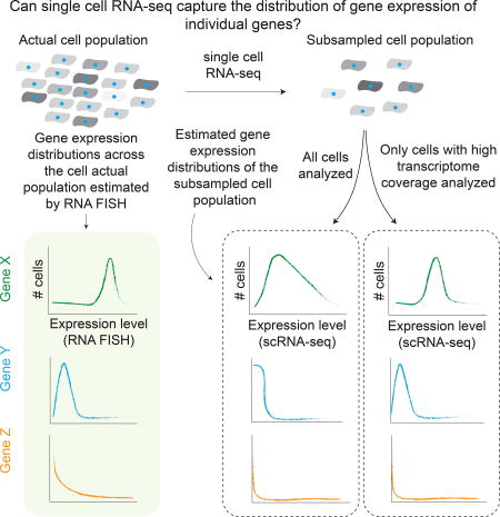
Figure 1. Technical sampling in single cell RNA sequencing can qualitatively change gene expression distributions.

(A) Single cell RNA sequencing (scRNA-seq) subsamples the actual transcriptome (left) to an observed transcriptome (middle). Different cells (horizontal rows) can have different degrees of transcriptome coverage. Depending on the number of cells analyzed, the observed expression distribution for any particular gene may not reflect the true distribution (right). We schematically depicted three classes of genes: high, minimally variable expression (GAPDH); low, minimally variable expression (SPP1); rare cells with high expression (NGFR). (B) Multiplexed single molecule RNA FISH is the gold standard for estimating gene expression at the single cell level. In each round of hybridization, we probe four genes, each with a set of DNA probes containing a common fluorophore. After imaging the resulting RNA spots, we strip the probes, and hybridize a new set of probes.

Here, we present a case study in single cell analysis which evaluates the tradeoff between number of cells analyzed, the depth to which each cell is sampled, and our ability to accurately recover distributions of single-cell expression patterns, focusing in particular on the identification and characterization of rare deviating cells in an isogenic population. Our previous work used single molecule RNA FISH (Fig. 1B) on many tens of thousands of cells to show that in melanoma cell lines, rare cells (that is, 1 in 50 to 500) express high levels (that is, dozens to hundreds of mRNA transcripts) of particular genes (e.g. EGFR, NGFR), and that this expression is associated with resistance to targeted therapy in this subset of cells (Shaffer et al. 2017). Here, the single molecule RNA FISH dataset serves as a gold standard distribution against which we compare single cell RNA sequencing data, and the distribution of gene expression across a population of cells that has a clear biological interpretation.

We performed single cell RNA sequencing using DropSeq and Fluidigm methodologies and evaluated our ability to detect rare cell expression at varying thresholds of transcriptome coverage (i.e. number of genes detected per cell). We demonstrate that in many experimental regimes, the apparent distributions of per-cell gene expression measured by single cell RNA sequencing and single molecule RNA FISH are dramatically different, that the observed distribution of cells in different states is dependent on transcriptome coverage, and that below an empirically-established threshold of transcriptome coverage, single cell RNA sequencing cannot reliably separate out genes with true rare cell expression from genes that were just poorly detected. Our approach provides an example of how to apply single cell sequencing techniques when single cell analysis is of the essence and technical demands are high due to the rarity of the behavior studied. We suggest that as the field begins evaluating techniques for large-scale data collection, it is a good time to consider the biological context and the requirements it imposes on both data generation and interpretation.

Results

We performed single cell analysis on a melanoma cell line, WM989-A6, a clonal isolate of the cell line WM989. This cell line serves as a model for melanoma therapy resistance: upon treatment with the BRAF inhibitor Vemurafenib, a subset of cells (around 1 in 2000 to 5000) continue to grow in the face of drug. In Shaffer et al. (Shaffer et al. 2017), we used multiplexed single molecule RNA FISH (Fig. 1B) to quantitatively measure the expression of resistance markers at the single cell level. We found that while these cells had overall low average expression of resistance markers such as EGFR, AXL, WNT5A and NGFR, occasional rare cells (around one in 50–500 cells) would express high levels of these genes. These rare cells were far more likely to be resistant to Vemurafenib.

To compare our existing RNA FISH dataset with single cell RNA sequencing, we used the WM989-A6-G3 cell line with both the DropSeq (Macosko et al. 2015) and Fluidigm (C1 mRNA Seq Ht IFC) platforms. Briefly, the DropSeq platform involves the production of droplets where individual cells lyse and their RNA binds to barcoded RNA-capture beads. The beads are then pooled for library preparation en masse. The Fluidigm platform captures cells in microfabricated wells, after which we performed library preparation as per the manufacturer’s recommendations, indeed, with the technical support person watching us very closely.

Single cell RNA sequencing inherently subsamples the transcriptome of each cell because the probability of recovery of any individual transcript is low (typically, only ~10% is recovered, (Marinov et al. 2014)). Moreover, the degree of subsampling is variable between cells. In principle, subsampling could have very different effects on the interpretation of expression variability from cell to cell depending on the expression level and underlying ground truth distribution. This is schematized on Figure 1A, which focuses on three genes, GAPDH, SPP1, and NGFR, and describes their actual expression and apparent expression after single cell RNA sequencing. The estimated distributions are all sensitive to the transcriptome coverage threshold, but the effect of thresholding on each distribution is specific to the pattern of expression of the gene. For instance, GAPDH, which expresses highly and ubiquitously, is relatively immune to this subsampling: decreasing transcriptome coverage thresholds increases the apparent variability in gene expression across the population, and the population mean might shift, but qualitatively, the distribution is similar. For other low but ubiquitously expressing genes (SPP1), however, there can be a qualitative change in which it appears as though they only express in rare cells. Meanwhile, true rarely expressing genes (e.g. NGFR) may not be detected at all. This thought experiment illustrates the challenge of imposing a threshold of transcriptome coverage for analysis and of inferring the true distribution of gene expression from single cell RNA sequencing data in the absence of a gold standard.

To illustrate these considerations experimentally, we measured the effect of subsampling on transcriptome coverage by observing the number of genes detected per cell(Fig. 2A). Effectively, this replaces the pie charts depicted in Figure 1A with experimentally-derived values. For our purposes, we defined transcriptome coverage as the number of unique genes detected per cell. To derive these values for DropSeq, we analyzed barcodes from individual beads. As expected, a large number of barcodes had very few reads, potentially due to sources of technical noise such as sequencing errors, barcode synthesis errors, and variability in the number of capture sites per bead. (Supp. Fig. 1 A). After we confirmed that most of our data represented transcriptomes from single cells rather than doublets (Supp. Fig. 1B), we selected the top 8600 cell barcodes for the remainder of the analysis, with a median sequencing depth of 6,938 uniquely mapped reads per cell and an interquartile range of 5,553 reads (Supp. Fig 1E). Ultimately, we obtained around 8000 cells with more than 500 genes detected per cell and around 1100 cells with more than 2000 genes detected per cell.

Figure 2. Averaging gene expression estimates across all cells in single cell RNA sequencing shows good correspondence across platforms.

(A) Distribution of transcriptome coverage (# genes detected per cell) for DropSeq (left) and Fluidigm (right). (B) Correlation of averaged gene expression estimates between single molecule RNA FISH (smRNA FISH) and single cell RNA sequencing (scRNA-seq). (C) Correlation of average gene expression estimates between DropSeq and smRNA FISH at different levels of transcriptome coverage using four different population sizes (50, 250, 500, and 2000 cells). Error bars in (C) represent ± 1 standard deviation across bootstrap replicates. (D) Correlation of averaged gene expression estimates between sequencing platforms. Error bars in (B and D) represent two times the standard error of the mean (SEM).

Fluidigm produced generally more evenly distributed transcriptomes, albeit with far fewer cells (335 out of a maximum possible of 800). Here, we sequenced the cells to a median depth of ~123,000 uniquely mapped reads per cell with an interquartile range of 110,642 reads (Supp. Fig. 1C,E).

For both platforms, an analysis of sequencing depth suggested that the transcriptome coverages we captured were not limited by the amount of sequencing we performed (Supp. Fig. 1D). Moreover, in both datasets, we detected ample expression of melanocyte markers and minimal expression of nonmelanocyte markers, providing confidence in the specificity of both datasets (Supp. Fig. 1F). The wide range of transcriptome coverages in our DropSeq data allowed us to explore the relationship between transcriptome coverage and various metrics of interest.

Out of a variety of metrics, we first looked at one we thought should be relatively insensitive to variability in transcriptome coverage: average gene expression. Despite the varying degrees of transcriptome coverage observed from cell to cell, if the subsampling is unbiased, pooling data from a large number of cells should lead to relative mean expression estimates that are insensitive to specific thresholds and similar across platforms. We pooled single cell RNA-seq data from all cells regardless of transcriptome coverage, and compared the resulting mean for each of 23–26 genes to the mean obtained by single molecule RNA FISH (Fig. 2B). We found that the correlation with single molecule RNA FISH was fairly strong for both single cell RNA sequencing methods (DropSeq R = 0.61; Fluidigm R = 0.63) (see also (Padovan-Merhar et al. 2015; Cabili et al. 2015)). Notably, this comparison includes several genes with low average expression due to the rarity of their expression. The reasonable correlation between Fluidigm, DropSeq, and single molecule RNA FISH data demonstrates that in our hands, single cell RNA sequencing is fairly effective at measuring average expression of even rarely expressed genes. As we expected, as the number of cells included in the analysis increased, so did the correlation between mean gene expression estimates (Fig. 2C). However, contrary to our predictions, we found the accuracy of mean gene expression estimates did depend on transcriptome coverage. For example, the estimate obtained from, say, 500 cells with an transcriptome coverage between 1,000–1,500 genes detected per cell yielded a higher correlation than the one obtained from the same number of cells with a shallower transcriptome coverage (e.g. 500–1000 genes detected per cell). This suggests that subsampling of a cell’s transcriptome is nonuniform.

While the correspondence between the single cell RNA sequencing data and single molecule RNA FISH was strong enough to capture trends, we wondered whether systematic differences between these approaches might be making the correspondence weaker than it otherwise would be. Therefore, we asked whether the correlation between datasets improves when exclusively compare sequencing-based techniques. To that end, we compared each single cell RNA sequencing dataset to bulk RNA sequencing data (DropSeq R = 0.94, Fluidigm R = 0.92) and compared Fluidigm and DropSeq to each other (R = 0.95)(Fig. 2D). Given the differences in RNA isolation and library preparation, and patterns of coverage between these methods of RNA sequencing, we concluded that the differences between single molecule RNA FISH and single cell RNA sequencing likely stem from systematic biases in sequencing and not from biases introduced by the different protocols. Accordingly, although the remainder of this study focuses mostly on data generated by DropSeq, we suggest that a similar approach may be taken to characterize Fluidigm data as well.

We next turned to the relationship between transcriptome coverage and the detection of rare cell expression variability. Two aspects of rare cell expression are a priori challenging for single cell RNA sequencing to detect. One is the detection of the rare cell with high levels of expression. The other is the discrimination of genes whose expression is not rare, but that appears to be rare due to the low capture efficiency of mRNA transcripts (Pierson and Yau 2015; H. Dueck et al. 2015; H. R. Dueck et al. 2016). A metric that is able to capture these effects is the Gini coefficient, developed by Corrado Gini as a means of quantifying income inequality. In the context of single cell expression levels (Jiang et al. 2016), a Gini coefficient of zero signifies an equal distribution of gene expression, whereas a Gini coefficient of one signifies the most extreme level of jackpot expression in which all the RNA is concentrated in a single cell while all the others have none. Intermediate Gini coefficients correspond to intermediate levels of heterogeneity (Fig. 3A). (We arrived at similar conclusions using the using the Kolmogorov–Smirnov (KS) statistic; Supp. Fig. 2A, B) The genes whose expression we analyzed by RNA FISH had Gini coefficients ranging from 0.29 to 0.98, with housekeeping genes such as GAPDH having a Gini coefficient of 0.33 while resistance markers like EGFR and WNT5A had Gini coefficients of 0.76 and 0.83.

Figure 3. Estimates of gene expression heterogeneity in single cell RNA sequencing are highly dependent on transcriptome coverage.

(A) The Gini coefficient measures a gene’s expression distribution and captures rare cell population heterogeneity. (B) Population structure of SOX10 mRNA levels measured by DropSeq (pink), Fluidigm (blue), and single molecule RNA FISH (smRNA FISH, brown). (C) Gini coefficient for six genes measured by DropSeq (left y-axis) binned by levels of transcriptome coverage as well as Gini coefficients measured by smRNA FISH (right y-axis). (D) Pearson correlation between Gini coefficients measured through DropSeq and smRNA FISH across different levels of transcriptome coverage (# genes detected per cell). Error bars represent ± 1 standard deviation across bootstrap replicates. (E,F) Scatter Plot of the correspondence between Gini coefficients for 26 genes measured by both DropSeq and smRNA FISH. (G) Scatter Plot of the correspondence between Gini coefficients for 26 genes measured by Fluidigm and smRNA FISH. (H) Pearson correlation between Gini coefficient estimates measured by DropSeq and smRNA FISH using different population sizes (# of cells) and levels of transcriptome coverage. Error bars represent ± 1 standard deviation across bootstrap replicates. (I) Pearson correlation between Gini coefficient estimates measured by DropSeq and smRNA FISH after subsampling cells with high transcriptome coverage to different degrees of reads depth. Numbers inside the bars represent the number of reads subsampled. The x-axis represents the average number of genes detected across all cells at a given subsample depth. Error bars represent ± 1 standard deviation across bootstrap replicates.

We then wondered how accurate single cell RNA sequencing measurements of Gini coefficients would be given the technical sensitivity of these platforms. We found that when we use very low thresholds for transcriptome coverage the Gini coefficient estimates from single cell RNA sequencing were generally higher than in single molecule RNA FISH; for instance, SOX10 has a Gini coefficient of 0.38 by single molecule RNA FISH, but has a Gini coefficient of 0.91 by DropSeq and 0.51 by Fluidigm (Fig. 3A). Practically, this means that the population distribution of SOX10 mRNA levels estimated by single cell RNA sequencing can be drastically different than the true distribution, as measured by single molecule RNA FISH (Fig. 3B).

Given that single cell RNA sequencing is often plagued by so-called zero inflation, in which some cells artificially have low or zero levels of many transcripts (H. Dueck et al. 2015; Pierson and Yau 2015; H. R. Dueck et al. 2016), likely inflating a Gini coefficient, we reasoned that accurate estimation of the Gini coefficient may depend on transcriptome coverage. To test this hypothesis, we binned the DropSeq dataset, which had cells of widely varying transcriptome coverages, by the number of genes detected per cell and computed the Gini coefficients for genes in which we had single molecule RNA FISH data (Fig. 3C). We found that the Gini coefficient estimates for genes with low variability (e.g. SOX10) generally decreased as transcriptome coverage increased, while the Gini estimates for highly variable genes (e.g. EGFR) remained high. For each of the bins, we then calculated the Pearson correlation coefficient between the Gini coefficient measured by single molecule RNA FISH and by DropSeq (Fig. 3D). We found that keeping only shallow cells yielded virtually no correlation, but cells with progressively more deep transcriptome coverage had increased correlation, with the correspondence increasing sharply until the number of genes detected per cell reached around 2000.

To see the effect more directly, we imposed two different stringency thresholds for transcriptome coverage, then asked whether the Gini coefficients for each resultant dataset matched those calculated from single molecule RNA FISH data. The correspondence with the Gini coefficients measured by single molecule RNA FISH was stronger when keeping only cells in which greater than 2000 genes were detected (Fig. 3E and F). Most of the improvement was driven by a drop in Gini coefficient for genes measured as more ubiquitously expressed by single molecule RNA FISH (Fig. 3E,F), suggesting that low capture efficiency of mRNA transcripts can artificially raise Gini coefficients when coverage isn’t sufficiently deep. However, although coverage depth does affect the accuracy of the calculated Gini coefficients, single cell RNA sequencing ranked genes according to their level of variability similarly to single molecule RNA FISH even at minimal coverage thresholds (Spearman correlations on Fig. 3E,F). At no point, though, is the correspondence between DropSeq and single molecule RNA FISH perfect, likely reflecting the statistical uncertainty inherent to measuring rare events. This suggests that while single cell RNA sequencing is able to discriminate qualitatively between variably and uniformly expressed genes, a threshold for transcriptome coverage of 2000 genes detected per cell (for our DropSeq data) was necessary for reasonably accurate quantification of rare cell expression. The Fluidigm dataset yielded similar correlations (Fig. 3G).

This analysis demonstrates that the improvement of Gini coefficient estimates from stringently filtering single cell RNA sequencing data is driven by decreases in artificially high Gini coefficients: as transcriptome coverage increases, Gini coefficients for genes that are uniformly expressed go down. This leads to the somewhat counterintuitive prediction that having a small number of cells with higher transcriptome coverage leads to more accurate Gini coefficients for rare cell expression than a large number of cells with shallow transcriptome coverage. We tested this prediction by estimating the Gini coefficient for a range of sample sizes (that is, number of cells included per sample) for cells binned by number of genes detected per cell (Fig. 3H). We found that increased sample size did improve the similarity of our Gini estimate with the single molecule RNA FISH estimate. However, we also found that using a large number of cells with low transcriptome coverage provided a worse estimate than using a small number cells of higher transcriptome coverage (e.g. compare n=50 cells with 1,500–2,000 genes detected to n=2000 with 500–1,000 genes detected, red arrows in Fig. 3H). This is because while including a large number of cells in the analysis increases the likelihood of detecting rare cells, these large datasets often include many cells with poor transcriptome coverage, which leads to many false positive rare cell expression events.

Poor transcriptome coverage leads to inaccurate Gini estimates. Given this observation, we wondered if this inaccuracy was simply a product of sequencing depth. In other words, is the difference between cells of high and low transcriptome coverage simply one of number of reads? To simulate the effect of sequencing depth (reads per cell) on the accuracy of Gini estimates, we subsampled cells with high transcriptome coverage (>2000 genes detected) to various degrees and then calculated the correlation coefficient between the Gini coefficient measured by single molecule RNA FISH and by single cell RNA sequencing, as well as the number of genes detected at the subsampled depth (Fig. 3I, Supp. Fig. 2C). For both subsampled (Fig. 3I) and un-subsampled (Fig. 3D) cells, the correspondence of Gini estimates decreased significantly below a coverage of 1,000 genes detected per cell. However the decrease is more precipitous in our actual dataset, suggesting that sequencing depth does not account for all the differences between cells of high and low transcriptome coverage.

In the analysis described above, single molecule RNA FISH data served as a gold standard to which single cell RNA sequencing data could be compared. This comparison defined how coverage depth and number of cells sampled affects the apparent distribution of per-cell gene expression; it also allowed us to determine appropriate thresholds of transcriptome coverage when detecting rare cells, our application of choice for this work. Next we asked whether an appropriate threshold for transcriptome coverage could be identified for a different application in the absence of a single molecule RNA FISH gold standard. Specifically, we asked whether we could use the cell cycle state to estimate this threshold.

The canonical view of the cell cycle is that at any given point, the number of cells cycling through each of the phases is not uniform: Mitosis is a short-lived, G1 is not (Fig. 4A). So, we expect a population to have many more cells in G1 than in Mitosis. We wondered what would be the required transcriptome coverage to recapitulate the expected distribution of cell cycle phases. To answer this question, we first classified each cell analyzed by DropSeq into a cell cycle phase (Fig. 4C, D left) based on its expression of a panel of genes known to be associated with different phases of the cell cycle (Whitfield et al. 2002). We also created a null expectation of randomly permuted data by shuffling, within each cell, the gene expression values of those genes that mark the different phases of the cell cycle. As expected, after randomizing the gene expression values of the cell cycle marker genes, the number of cells in each of the cycles appears to be relatively equal (Fig 4E, left), in disagreement with the canonical view of the cell cycle. The unshuffled dataset has a similarly equal distribution of cell cycle phases (Fig. 4C, left), suggesting that at minimal thresholds of transcriptome coverage we are unable to accurately classify cells into cell cycle phases any better than we would a randomly generated dataset.

Figure 4. Correct classification of single cells into multi-genic states is dependent on transcriptome coverage.

(A) Schematic depiction of the length of the cell cycle phases. (B) Calculation of a cell’s Signal Strength. (C) Percent of cells assigned to a cell cycle phase at different levels of transcriptome coverage (# genes detected per cell). (D, E) Heatmaps representing the correlation of a cell’s gene expression signature (columns) with each of the cell cycle phases (rows) for the DropSeq dataset (D) as well as for a null model (E) where the expression level of all cycling genes were randomly shuffled within each cell. We analyzed either all cells (left) or only cells with > 2,000 genes detected per cell (right). Below each heatmap is a representation of the proportion cells assigned to each phase of the cell cycle. Notice the length of each bar. (F) Signal strength across different levels of transcriptome coverage for DropSeq and a null model of randomized DropSeq data. Error bars represent ± 1 standard deviation across bootstrap replicates. (G) p-value of signal strength at different levels of transcriptome coverage using different number of genes to characterize the phase. Bar height indicates mean across bootstrap replicates. Error bars represent ± 1 standard deviation across bootstrap replicates.

To assess the relationship between transcriptome coverage and our ability to detect biological signal in the form of cell cycle phase distribution, we binned cells by the number of genes detected per cell, and then increased the stringency threshold and measured how signal emerged above the randomized control. We defined signal strength as the difference between how well a cell’s transcriptome correlated with the signature of the assigned phase and how well it correlated with the “opposite” phases (e.g., for a G2-assigned cell, how well it correlated with G2 minus how well it correlated with G1/S and M/G1 phases) (Fig. 4B). Our ability to detect cell cycle phase improved with the number of genes detected per cell. Moreover, we again found that at a threshold of around 2000 genes detected, the signal strength significantly increased above our randomized control (Fig. 4F), the number of cells in each phase fit more with the canonical view of the cell cycle, with most cells in G1 phase and less in G2 or M (Fig. 4C), and the classification of cells differed much more from randomized data, which continued to show an uniform distribution across phases. (Fig. 4D right and E right, see red arrows).

In the example above, we used 31–53 genes to infer cell cycle position. Next, we defined the relationship between the number of genes used to mark a specific cell cycle phase and our ability to classify that phase based on single cell RNA sequencing data. We classified cell cycle phase using random subsets of phase marker genes, for a range of transcriptome coverages (that is, genes detected per cell) (Fig. 4G). As expected, our ability to assign cell cycle phase based on signal strength increased with the number of marker genes available, while more subtle biological signals associated with fewer genes required higher transcriptome coverages to distinguish the signal from randomized data. For example, distinguishing a cell cycle phase based on the expression of 30 marker genes requires a transcriptome coverage of >1500 genes/cell, while a cell state defined by 20 marker genes requires >2500 genes/cell for the detection of any reliable signal (Fig. 4G, red arrows).

Discussion

We used a unique complementary set of data to assess how well single cell RNA sequencing is able to detect high levels of expression in rare cells. Our results suggest that with sufficient transcriptome coverage, single cell RNA sequencing is able to accurately discern rarely expressing genes from more ubiquitously expressing ones. These results highlight a tradeoff inherent to the analysis of single cell RNA sequencing data: how deep must the transcriptome coverage of a cell be before including it in the analysis?

Our results suggest that these choices strongly depend on the number of genes important for the biological question under consideration. Thus far, single cell RNA sequencing has mostly been used for cell type identification, which involves so many genes that it is relatively robust to low coverage transcriptomes. The rare cell phenotype we examined involved far fewer genes and thus was harder to detect with shallow transcriptomes, as did assignment of cell cycle phase.

As pointed out by Thomson et al. (Heimberg et al. 2016), the coverage of the transcriptome determines the conclusions one is able to make, and as the number of genes involved in the biology in question decreases, the coverage required will generally increase. For example, cell types typically differ in the expression of thousands of genes, making it relatively easy to discriminate between them even with shallow transcriptomes, even if the cell type is rare (Grün et al. 2015). However, accurately measuring, for example, the cell-to-cell variability in expression of a single gene requires having deep transcriptome coverage to ensure accurate transcript quantification in each cell. In general, most biological processes lie somewhere in between these extremes, and the specifics of the process (e.g. number of genes involved) may impose a particular structure on the data that may or may not be captured at a particular transcriptome coverage.

Given this context, it is important to realize that transcriptome coverage is just one of a number of technical metrics that may be important for evaluating single cell RNA sequencing-based approaches to answer any particular biological question. Such considerations will also be important for image-based techniques, where confounders such as cell size (Padovan-Merhar et al. 2015; Battich, Stoeger, and Pelkmans 2015; Kempe et al. 2015) and others can also affect biological interpretations (Cote et al. 2016). We think that as the field moves towards answering particular biological questions with single cell RNA sequencing and other single cell technologies, it will be increasingly important to perform comparative studies, ideally with gold standards, to evaluate the ability to make robust claims.

At the same time, new computational tools such as MAGIC (van Dijk et al. 2017) are under development that aim to recover correlations from shallow-coverage cells in single cell RNA sequencing datasets, as well as tools like SAVER (Huang et al., n.d.) that are even able to recover distributions of gene expression from shallow-coverage cells. SAVER is able to recover these distributions by training a prediction model across all cells regardless of coverage, thus yielding counts per cell based on a weighted average of the model prediction and the experimental observations. It remains to be seen how much these methods rely on the particulars of the distribution of transcriptome coverage across cells. It also may be that hybrid depth-studies, with a smaller subset of cells at very high transcriptome coverage and a large set of cells at shallow transcriptome coverage, may prove useful, with the former discriminating which genes express ubiquitously and the latter finding those that express rarely.

STAR Methods

CONTACT FOR REAGENT AND RESOURCE SHARING

Further information and requests for resources and reagents should be directed to and will be fulfilled by the Lead Contact, Arjun Raj (arjunraj@seas.upenn.edu).

EXPERIMENTAL MODEL AND SUBJECT DETAILS

Human Melanoma Cells

We obtained WM989 melanoma cells (female) from the lab of Meenhard Herlyn (M.H.) and derived A6 and A6-G3 single cell subclones in our lab. We grew these cells at 37C in Tu2% media (78% MCDB, 20% Leibovitz’s L-15 media, 2% FBS, and 1.68mM CaCl2). This cell line was fingerprinted in the lab of M.H. by short tandem repeat profiling using AmpFlSTR Identifiler PCR Amplification Kit (Life Technologies).

Mouse Cells

We grew 3T3 murine cells (male) at 37C in DMEM media (10% FBS, 0.5% pen/strep), and murine JC4 (undetermined sex, single × chromosome) suspension cells at 37C in IMDM media (10% FBS, 2% pen/strep, 50 ng/ml Kit ligand, 2 U/ml erythropoietin, 4.5 × 10^-5 M monothioglycerol). We did not fingerprint these cells. In our analysis they were used only to track rate of doublets in Dropseq.

METHOD DETAILS

Single molecule RNA FISH

For single molecule RNA FISH we seeded cells in two-well LabTek chambered coverglasses and cultured them to ~50–70% confluency. We performed single molecule RNA FISH and high-throughput microscopy scans as previously described (Raj et al. 2008; Shaffer et al. 2017). In short, we first fixed adherent cells with 4% formaldehyde in PBS for 10 min at RT and permeabilized with 70% EtOH at 4C overnight. We hybridized FISH probes (DNA oligonucleotides conjugated to fluorescent dyes, Supplemental Table 4) overnight at 37C, washed away unbound probes, and stained DNA with DAPI prior to acquiring a tiled grid of images. Note that in our imaging system, we measured expression in a single z-plane of the cell; thus, the exact numbers for each cell are not total mRNA counts per cell, but rather an amount proportional to the total. For iterative FISH, we stripped DNA probes and hybridized new ones as in Shaffer et. al. (Shaffer et al. 2017). In short, after an initial round of imaging, we removed bound DNA probes using 60% formamide in 2× SSC during a 15 minutes incubation at 37C. We then removed the formamide with three 15-minute PBS washes at 37C. Finally, we washed one last time with wash buffer prior to adding a new set of DNA probes. For more details on how to make buffers for RNA FISH and on how to carry out the experiments please visit: https://sites.google.com/site/singlemoleculernafish/

DropSeq

We generated single cell suspensions by trypsinizing adherent cells with 0.05% trypsin-EDTA or by harvesting suspensions cells. We passed all cells through a 40 micron filter and diluted them to 100 cells/ul in 0.01% PBS-BSA. We carried out all subsequent steps as detailed by Macosko et. al, protocol v3.1 (http://mccarrolllab.com/dropseq/). In short, we loaded cells in 0.01% PBS-BSA and barcoded beads (chemgenes Barcoded Bead SeqB, cat. No. MACOSKO-2011-10) in lysis buffer onto a droplet generating microfluidic device. After breaking the droplets, we pooled the beads into aliquots of ~60,000, reverse transcribed the RNA captured by the barcoded beads, and digested unbound poly-dT tails via exonuclease treatment. We PCR-amplified STAMPs (2000 beads per reaction), purified cDNA using AMPure beads and quantified the library via Agilent’s High Sensitivity DNA Chip. We then tagmented the resulting cDNA with Nextera XT adapters and purified the final library with Ampure beads. We sequenced all libraries using Nextseq 500 with the custom Dropseq read 1 primer described by Macosko et. al.

Fluidigm C1 mRNA Sequencing

To prepare single cell suspensions, we dissociated WM989-A6-G3 cells as above. We immunostained the cells as per Shaffer et. al (Shaffer et al. 2017). Briefly, we incubated cells for 1 hour at 4C with 1:200 mouse anti-EGFR antibody, clone 225 (Millipore, MABF120) in 0.1% BSA PBS. We then washed twice with 0.1% PBS-BSA and then incubated for 30 minutes at 4C with 1:500 donkey anti-mouse IgG-Alexa Fluor488 (Jackson Laboratories, 715-545-150). We washed the cells again (twice) with 0.1% BSA-PBA and incubated for 10 minutes with 1:500 anti-NGFR APC-labelled clone ME20.4 (Biolegend, 345107). After we washed the cells with 0.1% BSA-PBS and pelleted them, we resuspended them in Tu2%, passed them through a 35 micron filter, and diluted them to a final concentration of ~350 cells per ul in Tu2%. We prepared the samples and sequencing library according to the manufacturer’s instructions (https://www.fluidigm.com/products/c1-system). In short, we loaded and captured single cells on Fluidigm’s C1 integrated fluidic circuit and inspected the capture chambers via microscopy. We then lysed the cells, barcoded the captured mRNA via RT with a barcoded primer, and amplified the resulting cDNA via PCR. Unlike DropSeq, this protocol uses no unique molecular identifiers to label RNA molecules. After we harvested the amplified cDNA, we tagmented the library using Nextera’s XT DNA sample preparation kit (following Fluidigm’s version of the protocol), purified the final library using Ampure beads and quantified using Agilent’s High Sensitivity DNA Chip. We sequenced the library using a Nextseq 500.

Bulk RNA sequencing

We sequenced mRNA in bulk from WM989-A6 populations as per Shaffer et. al. We isolated mRNA and built sequencing libraries using the NEBNext Poly(A) mRNA Magnetic Isolation Module and NEBNext Ultra RNA Library Prep Kit for Illumina. We sequenced the libraries either on a HiSeq 2000 or a NextSeq 500 to a depth of approximately 20 million reads.

QUANTIFICATION AND STATISTICAL ANALYSIS

Drop-seq alignment and quantification

Initial Drop-seq data processing was performed using Drop-seq_tools-1.0.1 (http://mccarrolllab.com/dropseq/), and following protocol described in seqAlignmentCookbook_v1.1Aug2015.pdf, accessed from the same site. Data were aligned using STAR version 2.4.2a, downloaded from github on Jan 21, 2016. Data were aligned to reference genome builds hg38 (Human) and mm10 (Mouse), and using reference transcriptome annotations Gencode21 (Human) and Refseq mm10 (Mouse), concatenated with ERCC sequences. Reference transcriptome annotations Gencode21 (Human) and Ensembl mm10 release 83 (Mouse), concatenated with ERCC annotations. Briefly, reads with low-quality base in either cell or molecular barcode were filtered and reads were trimmed for contaminating primer or poly-A sequence. Sequencing errors in barcodes were inferred and corrected, as implemented by Drop-seq_tools-1.0.1. Uniquely mapped reads, with <= 1 insertion or deletion, were used in quantification. To account for differences in molecule recovery, cell measurements were normalized to UMI per million (UPM).

Fluidigm alignment and quantification

Fluidigm sequence data were demultiplexed using mRNASeqHT_demultiplex.pl (https://www.fluidigm.com/c1openapp/scripthub/script/2015-08/mrna-seq-ht-1440105180550-2). Demultiplexed data were processed in the same manner as Drop-seq data, with a few modifications: 5’ ends of reads were not trimmed, and reads (rather than UMI) were used for quantification. To account for differences in molecule recovery and sequencing depth, cell measurements were normalized to reads per million (RPM).

Bulk sequencing alignment and quantification

We aligned reads to hg19 and quantified reads per gene using STAR and HTSeq.

Single molecule RNA FISH quantification

All image analysis was performed as per Shaffer et. al. (Shaffer et al. 2017). We developed a MATLAB analysis pipeline (freely available here https://bitbucket.org/arjunrajlaboratory/rajlabimagetools/wiki/Dentist) that segments nuclei of individual cells using DAPI images. The pipeline then identifies regional maxima as potential RNA FISH spots and assigns them to the nearest nuclei. We then select a signal intensity threshold for each RNA FISH channel to differentiate background from RNA FISH signal and manually curate the dataset to eliminate imaging artifacts that the software recognizes as RNA FISH signal. We then extract the position of every cell in the scan and the number of RNA molecules for each fluorescent channel. To match cells across subsequent hybridizations, we developed software that shifts cells in the first hybridization to all potential candidates in the subsequent hybridization (Shaffer et al. 2017). It then chooses the best match as the one that minimizes the total distance for nearby cells. We then matched cells by proximity and discarded those cells that did not match uniquely to a nearby cell.

Selecting quality single cell Drop-seq data

Cell barcodes were classified as quality human cells, based on the following criteria: 1) Greater than 80% of species-specific transcripts were assigned to human, and at least 100 species-specific transcripts were available for assignment. 2) The cell barcode was not assigned a synthesis error. The remaining barcodes were filtered to retain the expected number of cells. Based on experiment, we expected 8640 single human cells, and we retained the 8640 cell barcodes with largest read depth (Supplemental Table 1).

Selecting quality single cell Fluidigm data

The Fluidigm system allowed cells to be imaged before processing, and for images to be associated with sequencing data. In our automated setup, not all wells were imaged, and well numbers were not captured in images (though column identity on the chip was known). In order to use images to identify quality single cells, we first re-ordered visual annotations to best match read depth observed per well (so that images of empty wells had low depth compared to images with individual or multiple cells). Given re-ordered images, wells were classified as quality single cells if: 1) based on associated image, the well was annotated as containing a good, single cell, and 2) if the cell appeared to be distinct from wells annotated as empty by read depth. Both criteria were required (Supplemental Tables 2 and 3).

Sufficiency of sequencing depth

We wanted to ensure that our metric of library coverage (number of genes observed) did not reflect sequencing depth. To test whether the Drop-Seq and Fluidigm experiments were sequenced to a sufficient depth, we examined the relationship between experimental read depth and the average number of genes observed in single cells. To do this, we randomly and uniformly subsampled reads from the Drop-seq (or Fluidigm) read counts table, for a variety of experimental sequencing depths. We generated 10 random samples at each sequencing depth, and report the average number of observed genes, across cells and sample replicates. We generated random samples for an average depth per cell of 100, 500, and 1000 – 500,000 (step size of 1000) raw reads per cell. (For Drop-seq data, our experimental depth allowed testing depths up to 120,000 average raw reads per cell.) To identify the number of reads to subsample from the read count table, given these raw read depths per cell, we calculated the fraction of all sequenced reads that were assigned to the read count table. At each selected experimental depth, we used this fraction of reads to subsample the read counts table. For Dropseq data, 11.2% of raw reads were uniquely assigned to genes in quality cells. In Fluidigm data, 29.3% of reads were uniquely assigned to genes in quality cells.

Tissue-marker gene expression

We selected tissue marker genes for melanocytes, pancreas, heart, and spleen from TIGER (http://bioinfo.wilmer.jhu.edu/tiger/). For each tissue type the genes were selected for analysis based on the expression level in their respective tissue and their presence in both single cell RNA sequencing datasets.

Comparison of average measurements

We calculated mean ± 2 SEM for each measurement type. Two genes with RNA FISH measurements were excluded (VGF and NGFR) due to difficulty in quantifying the RNA FISH measurements. One additional gene (AXL) was not observed in the Fluidigm data, and was excluded from Fluidigm comparison. Pearson and Spearman correlations were calculated over genes observed in both Drop-seq and Fluidigm and were calculated on a log₁₀ scale.

Filtering and normalization for calculation of rare cell variability

It has been shown that a portion of molecular variability across single cells is due to cell volume (Padovan-Merhar et al. 2015). To focus on rare cell variability, we normalized single molecule RNA FISH cells to GAPDH, using GAPDH levels as a proxy for cell volume. Cells with <50 GAPDH molecules observed were filtered prior to normalization. For visualization, we scaled normalized values by 400 so that normalized counts were on roughly the same scale as single cell molecule counts. In order that sequencing data remain comparable to single molecule RNA FISH data, we filtered Drop-seq and Fluidigm cells with no observed GAPDH. We then scaled the (sequencing-depth normalized) Drop-seq and Fluidigm data so that the median GAPDH level across cells was 400, so that sequencing measurements were on a similar scale to single molecule RNA FISH measurements.

Measure of rare cell variability

Gini coefficients were calculated using the R package “ineq”.

Effect of library coverage on Gini coefficient estimate

To test the effect of library coverage on estimates of population statistics, we binned cells by library coverage, using the number of observed genes as our metric of coverage. We used bins ranging from 0 to 5500 observed genes, with a step size of 500 genes. Sample size (the number of cells in a bin) is expected to affect the estimate of the Gini coefficient. We controlled for sample size (number of cells) by randomly subsampling cells within a bin, to reach 50 cells per bin, prior to calculating the Gini coefficient. Random sampling was repeated 100 times per bin. So that normalization was consistent across all random subsamples, we normalized all cells to cellular GAPDH level. As previously, single molecule RNA FISH cells with <50 GAPDH molecules were excluded, as were Drop-seq and Fluidigm cells with no GAPDH observed. For each coverage bin, we calculated the Pearson correlation of Gini coefficient estimates calculated on Drop-seq data with those calculated using single molecule RNA FISH data. For each bin, we report the average correlation across subsample replicates ± 1 standard deviation.

Effect of read number on Gini coefficient estimate

To evaluate dependence of Gini coefficient estimates on sequencing depth, we randomly subsampled cells containing > 2,000 genes detected per cell to various read depths (500, 1000, 2000, 3000, 4000, 5000, 6000, 7000, 8000, 9000, 10000, 11000, and 12000 reads per cell). We repeated random subsampling ten times at each depth. Then, for those genes for which we had RNA FISH data, we obtained GAPDH-normalized gene expression estimates and Gini coefficients. At each subsampling depth and for each replicate we obtained a pearson correlation of the Gini coefficients between RNA FISH and scRNA-seq. For each read depth we report the average correlation across all subsample replicates ± 1 standard deviation.

Effect of sample size (number of cells) on Gini coefficient estimate

To evaluate the effect of sample size on Gini coefficient estimates, we repeated the analysis described above for a variety of numbers of cells for each coverage bin.

Cell cycle phase classification

To assess our ability to detect biological expression patterns using Drop-seq and Fluidigm measurements, we assigned cell cycle phase to individual cells, following the approach used in Macosko et al. (Macosko et al. 2015) and using cell cycle marker genes identified in Whitfield et al. (Whitfield et al. 2002). The Macosko et al. approach involves the following steps: 1) Marker genes were filtered to exclude genes that do not cycle in melanoma cells. For each set of genes assigned to a particular cell cycle phase, the average expression profile was calculated across the data set. For each individual gene within that set, the correlation with this average profile was calculated. Genes with correlation <0.3, in either Drop-seq or Fluidigm data, were excluded. 2) Depth-normalized read counts were zero-adjusted and log₂ normalized. 3) For each cell and phase, a phase score was assigned by calculating the average normalized value across marker genes for that phase. 4) Phase scores were z-normalized, first across cells within each phase, and then across phases within each cell. 5) Sample phase was assigned to each cell. To do this, a binary score profile was created for idealized cells at each phase and phase transition. The correlation of a cell’s normalized score profile with this set of idealized profiles was calculated. A cell was assigned a phase based on the maximum observed correlation.

Effect of library coverage on cell cycle phase classification

To test the effect of library coverage on cell phase classification, we binned cells by the number of observed genes as described above and, as above, we controlled for sample size (number of cells) by randomly subsampling cells within a bin, to reach 50 cells per bin. For each set of sampled cells, we classified cell cycle phase as described above. To generate a random expectation for cell cycle phase categorization, we generated 1000 random counts tables, shuffling counts across cell cycle marker genes for each sample. For each table, we proceeded with cell cycle phase classification as described above. We used the same sets of samples as used in test data, so that each tested population of cells was compared to a biologically and technically matched population with randomized expression profiles.

To summarize the strength of biological signal, we calculated for each cell the best correlation with an idealized phase profile (the assigned phase for the cell) and the best correlation with an idealized phase profile for an “off” phase, or a cell cycle phase that does not neighbor the assigned phase. We report the difference between these correlations. To provide a population-level statistic, we calculate the average strength of biological system for each tested population (each randomly sampled set of 50 cells). To assess the significance of this statistic, we calculated the same statistic for each null (randomly shuffled) population, and report the fraction of times that a signal as large or larger is observed. Finally, we summarize these results across the randomly sampled populations (the random sets of 50 cells), reporting the average ± 1 standard deviation across subsample replicates.

Effect of number of marker genes on cell cycle phase classification

To evaluate the effect of the number of available marker genes, we repeated the analysis described above for a variety of numbers of genes. We randomly selected n marker genes for each phase (n from 1 to 30), and then ran the analysis described above on that subset of genes. We repeated this 100 times for each n. For randomized data, we selected n genes for each phase once, because the identity of the gene has been lost in randomizing the data. (This means each of the 1000 randomized replicates is essentially a different random gene set sample as well.) So, each of the 100 replicates of test data for a given n are compared to the same null expectation.

NOTE: All statistical details for a given analysis, including definition of center and dispersion measurements, and exact value of n are detailed in the figures.

DATA AND SOFTWARE AVAILABILITY

• -The raw datasets from DropSeq and Fluidigm have been deposited in the GEO repository under accession number GSE99330. They can also be found at: https://www.dropbox.com/sh/tjdv3mgxle30qiv/AAAXdnYJRZzMeZYaQg7YIUUaa?dl=0
• -The raw reads obtained through bulk RNA sequencing can be found at: https://www.dropbox.com/s/ir7fp9ragta8jan/A6_bulk_NoDrug.fastq.gz?dl=0
• -The code used for analysis throughout the paper can be found at: https://www.dropbox.com/sh/scmiu1tbrsxupto/AACTL5iWaW-zxRmAbFXnIwnMa?dl=0
• -The single molecule RNA FISH data file as well as the code used for analysis can be found at: https://www.dropbox.com/sh/g9c84n2torx7nuk/AABZei_vVpcfTUNL7buAp8z-a?dl=0

Supplementary Material

1

Supplemental Figure 1. Related to Figure 2. (A) Distribution of reads across all barcodes sequenced in DropSeq represented as the number of cell barcodes containing a given number of uniquely mapped reads (main figure), and the cumulative fraction of reads as a function of the number of barcodes (inset). (B) Scatterplot representing the number of human and mouse transcripts associated with each cell barcode in the DropSeq dataset. (C) Distribution of reads across a capture chamber in Fluidigm's platform (top left), example of a single cell (yellow) as well as a cell clump (blue) inside the cell capture chambers (right), and proportion of cell capture chambers containing a single cell (bottom left). (D) Sequencing coverage assessed as the number of genes detected per cell as a function of the number of reads obtained for each cell for DropSeq (left) and Fluidigm (right). (E) Sequencing statistics for libraries built with DropSeq (n = 1 biological replicate) and Fluidigm (n = 1 biological replicate). This table is not meant to serve as a comparison between single cell RNA sequencing methods. We did not optimize either platform for such a comparison. (F) Gene expression estimates of tissue-marker genes for DropSeq (left) and Fluidigm (right).

Supplemental Figure 2. Related to Figure 3. (A) Comparison of the gene expression distribution (Kolmogorov-Smirnov statistic) for five genes (LMNA, SOX10, MITF, EGFR, and WNT5A) measured by DropSeq and single molecule RNA FISH (smRNA FISH). We measured the KS statistic across different levels of transcriptome coverage (# genes detected per cell). Unless otherwise indicated, at each level of transcriptome coverage the KS test was repeated 100 times, each time randomly sampling 50 cells from the population. The distribution of KS values across bootstrap replicates is depicted as a boxplot. (B) Median KS statistic between DropSeq and single molecule RNA FISH of 26 genes across varying degrees of transcriptome coverage. Bar height indicates the average across bootstrap replicates. Error bars represent ± 1 standard deviation across bootstrap replicates. (C) Correlation between Gini coefficient estimates measured by Fluidigm and single molecule RNA FISH after subsampling cells with high transcriptome coverage to different degrees of reads depth. The numbers inside the bars represent the number of reads subsampled. The average number of genes detected across all cells at a given subsample depth is reported in the x-axis. Error bars represent ± 1 standard deviation across bootstrap replicates.

2

Table 1: Selected DropSeq cell barcodes. Related to STAR methods.

3

Table 2: Selected Fluidigm cell barcodes. Related to STAR methods.

4

Table 3. Visual annotations for Fluidigm dataset. Related to STAR methods.

5

Table 4. RNA FISH probes. Related to STAR methods.

KEY RESOURCES TABLE

REAGENT or RESOURCE	SOURCE	IDENTIFIER
Antibodies
mouse anti-EGFR antibody, clone 225	Millipore	MABF120
anti-mouse IgG-Alexa Fluor488	Jackson Laboratories	715-545-150
anti-NGFR APC-labelled clone ME20.4	Biolegend	345107
Bacterial and Virus Strains
N/A	N/A	N/A
Biological Samples
N/A	N/A	N/A
Chemicals, Peptides, and Recombinant Proteins
N/A	N/A	N/A
Critical Commercial Assays
C1 single cell mRNA seq IFC	Fluidigm	100–5760
NEBNext Poly(A) mRNA Magnetic Isolation Module	NEB	E7490S
NEBNext Ultra RNA Library Prep Kit for Illumina	NEB	E7530S
Deposited Data
Raw Single cell RNA seq data	this paper	https://www.dropbox.com/sh/tjdv3mgxle30qiv/AAAXdnYJRZzMeZYaQg7YIUUaa?dl=0; GSE99330
Raw Bulk RNA seq data	Shaffer et al. 2017	https://www.dropbox.com/s/ir7fp9ragta8jan/A6_bulk_NoDrugfastq.gz?dl=0
RNA FISH data	Shaffer et al. 2017	https://www.dropbox.com/s/om8uq3z3lxnfdtk/fishSubset.txt?dl=0
Experimental Models: Cell Lines
WM989	Meenhard Herlyn	N/A
NIH 3T3	Raj Lab	N/A
JC4	Raj Lab	N/A
Experimental Models: Organisms/Strains
N/A	N/A	N/A
Oligonucleotides
RNA FISH Probe sequences	Biosearch Technologies	Supplementary Table 4
Recombinant DNA
N/A	N/A	N/A
Software and Algorithms
RNA FISH image analysis software	Raj Lab	https://bitbucket.org/arjunrajlaboratory/rajlabimagetools/wiki/Dentist
scRNA-seq analysis code	This paper	https://www.dropbox.com/sh/scmiu1tbrsxupto/AACTL5iWaW-zxRmAbFXnIwnMa?dl=0
Drop-seq_tools-1.0.1	McCaroll Lab	http://mccarrolllab.com/dropseq/
STAR version 2.4.2a		https://github.com/alexdobin/STAR/releases
mRNASeqHT_demultiplex.pl		https://www.fluidigm.com/c1openapp/scripthub/script/2015-08/mrna-seq-ht-1440105180550-2
HTSeq		https://pypi.python.org/pypi/HTSeq
Other
N/A	N/A	N/A

Highlights.

• -Estimates of rare cell gene expression vary with transcriptome coverage
• -The no. of cells analyzed also affects estimates of rare cell gene expression
• -In rare cell analysis, cell coverage has a larger effect than the no. of cells used
• -Internal and external controls guide selection of transcriptome coverage thresholds

References

- Battich Nico, Stoeger Thomas, Pelkmans Lucas. Control of Transcript Variability in Single Mammalian Cells. Cell. 2015;163(7):1596–1610. doi: 10.1016/j.cell.2015.11.018. [DOI] [PubMed] [Google Scholar]
- Brennecke Philip, Anders Simon, Kim Jong Kyoung, Kołodziejczyk Aleksandra A, Zhang Xiuwei, Proserpio Valentina, Baying Bianka, et al. Accounting for Technical Noise in Single-Cell RNA-Seq Experiments. Nature Methods. 2013;10(11):1093–95. doi: 10.1038/nmeth.2645. [DOI] [PubMed] [Google Scholar]
- Cabili Moran N, Dunagin Margaret C, McClanahan Patrick D, Biaesch Andrew, Padovan-Merhar Olivia, Regev Aviv, Rinn John L, Raj Arjun. Genome Biology. 1. Vol. 16. BioMed Central Ltd; 2015. Localization and Abundance Analysis of Human lncRNAs at Single-Cell and Single-Molecule Resolution; p. 20. [DOI] [PMC free article] [PubMed] [Google Scholar]
- Cote Allison J, McLeod Claire M, Farrell Megan J, McClanahan Patrick D, Dunagin Margaret C, Raj Arjun, Mauck Robert L. Nature Communications. March. Vol. 7. Nature Publishing Group; 2016. Single-Cell Differences in Matrix Gene Expression Do Not Predict Matrix Deposition; p. 10865. [DOI] [PMC free article] [PubMed] [Google Scholar]
- Dijk David van, Nainys Juozas, Sharma Roshan, Kathail Pooja, Carr Ambrose J, Moon Kevin R, Mazutis Linas, Wolf Guy, Krishnaswamy Smita, Pe’er Dana. MAGIC: A Diffusion-Based Imputation Method Reveals Gene-Gene Interactions in Single-Cell RNA-Sequencing Data. bioRxiv. 2017 doi: 10.1101/111591. [DOI]
- Dueck Hannah, Eberwine James, Kim Junhyong. Variation Is Function: Are Single Cell Differences Functionally Important? BioEssays: News and Reviews in Molecular, Cellular and Developmental Biology. 2016;38(2):172–80. doi: 10.1002/bies.201500124. [DOI] [PMC free article] [PubMed] [Google Scholar]
- Dueck Hannah, Khaladkar Mugdha, Kim Tae Kyung, Spaethling Jennifer M, Francis Chantal, Suresh Sangita, Fisher Stephen A, et al. Deep Sequencing Reveals Cell-Type-Specific Patterns of Single-Cell Transcriptome Variation. Genome Biology. 2015;16(June):122. doi: 10.1186/s13059-015-0683-4. [DOI] [PMC free article] [PubMed] [Google Scholar]
- Dueck Hannah R, Ai Rizi, Camarena Adrian, Ding Bo, Dominguez Reymundo, Evgrafov Oleg V, Fan Jian-Bing, et al. Assessing Characteristics of RNA Amplification Methods for Single Cell RNA Sequencing. BMC Genomics. 2016;17(1):966. doi: 10.1186/s12864-016-3300-3. [DOI] [PMC free article] [PubMed] [Google Scholar]
- Grün Dominic, Kester Lennart, van Oudenaarden Alexander. Validation of Noise Models for Single-Cell Transcriptomics. Nature Methods. 2014;11(6):637–40. doi: 10.1038/nmeth.2930. [DOI] [PubMed] [Google Scholar]
- Grün Dominic, Lyubimova Anna, Kester Lennart, Wiebrands Kay, Basak Onur, Sasaki Nobuo, Clevers Hans, van Oudenaarden Alexander. Nature. 7568. Vol. 525. Nature Publishing Group; 2015. Single-Cell Messenger RNA Sequencing Reveals Rare Intestinal Cell Types; pp. 251–55. [DOI] [PubMed] [Google Scholar]
- Heimberg Graham, Bhatnagar Rajat, El-Samad Hana, Thomson Matt. Cell Systems. 4. Vol. 2. Elsevier; 2016. Low Dimensionality in Gene Expression Data Enables the Accurate Extraction of Transcriptional Programs from Shallow Sequencing; pp. 239–50. [DOI] [PMC free article] [PubMed] [Google Scholar]
- Huang M, Wang J, Torre E, Dueck H, Shaffer S, Bonasio R, Murray J, Raj A, Li M, Zhang NR. Gene Expression Recovery for Single Cell RNA Sequencing. doi: 10.1038/s41592-018-0033-z. n.d. [DOI] [PMC free article] [PubMed] [Google Scholar]
- Jiang Lan, Chen Huidong, Pinello Luca, Yuan Guo-Cheng. GiniClust: Detecting Rare Cell Types from Single-Cell Gene Expression Data with Gini Index. Genome Biology. 2016;17(1):144. doi: 10.1186/s13059-016-1010-4. [DOI] [PMC free article] [PubMed] [Google Scholar]
- Kempe Hermannus, Schwabe Anne, Crémazy Frédéric, Verschure Pernette J, Bruggeman Frank J. The Volumes and Transcript Counts of Single Cells Reveal Concentration Homeostasis and Capture Biological Noise. Molecular Biology of the Cell. 2015;26(4):797–804. doi: 10.1091/mbc.E14-08-1296. [DOI] [PMC free article] [PubMed] [Google Scholar]
- Kolodziejczyk Aleksandra A, Kim Jong Kyoung, Svensson Valentine, Marioni John C, Teichmann Sarah A. The Technology and Biology of Single-Cell RNA Sequencing. Molecular Cell. 2015;58(4):610–20. doi: 10.1016/j.molcel.2015.04.005. [DOI] [PubMed] [Google Scholar]
- Macosko Evan Z, Basu Anindita, Satija Rahul, Nemesh James, Shekhar Karthik, Goldman Melissa, Tirosh Itay, et al. Highly Parallel Genome-Wide Expression Profiling of Individual Cells Using Nanoliter Droplets. Cell. 2015;161(5):1202–14. doi: 10.1016/j.cell.2015.05.002. [DOI] [PMC free article] [PubMed] [Google Scholar]
- Marinov Georgi K, Williams Brian A, McCue Ken, Schroth Gary P, Gertz Jason, Myers Richard M, Wold Barbara J. From Single-Cell to Cell-Pool Transcriptomes: Stochasticity in Gene Expression and RNA Splicing. Genome Research. 2014;24(3):496–510. doi: 10.1101/gr.161034.113. [DOI] [PMC free article] [PubMed] [Google Scholar]
- Padovan-Merhar Olivia, Nair Gautham P, Biaesch Andrew G, Mayer Andreas, Scarfone Steven, Foley Shawn W, Wu Angela R, Churchman L Stirling, Singh Abhyudai, Raj Arjun. Single Mammalian Cells Compensate for Differences in Cellular Volume and DNA Copy Number through Independent Global Transcriptional Mechanisms. Molecular Cell. 2015;58(2):339–52. doi: 10.1016/j.molcel.2015.03.005. [DOI] [PMC free article] [PubMed] [Google Scholar]
- Pierson Emma, Yau Christopher. ZIFA: Dimensionality Reduction for Zero-Inflated Single-Cell Gene Expression Analysis. Genome Biology. 2015 doi: 10.1186/s13059-015-0805-z. [DOI] [PMC free article] [PubMed]
- Raj Arjun, van den Bogaard Patrick, Rifkin Scott A, van Oudenaarden Alexander, Tyagi Sanjay. Nature Methods. 10. Vol. 5. Nature Publishing Group; 2008. Imaging Individual mRNA Molecules Using Multiple Singly Labeled Probes; pp. 877–79. [DOI] [PMC free article] [PubMed] [Google Scholar]
- Raj Arjun, van Oudenaarden Alexander. Nature, Nurture, or Chance: Stochastic Gene Expression and Its Consequences. Cell. 2008;135(2):216–26. doi: 10.1016/j.cell.2008.09.050. [DOI] [PMC free article] [PubMed] [Google Scholar]
- Shaffer Sydney M, Dunagin Margaret C, Torborg Stefan R, Torre Eduardo A, Emert Benjamin, Krepler Clemens, Beqiri Marilda, et al. Nature. 7658. Vol. 546. Nature Research; 2017. Rare Cell Variability and Drug-Induced Reprogramming as a Mode of Cancer Drug Resistance; pp. 431–35. [DOI] [PMC free article] [PubMed] [Google Scholar]
- Shapiro Ehud, Biezuner Tamir, Linnarsson Sten. Single-Cell Sequencing-Based Technologies Will Revolutionize Whole-Organism Science. Nature Reviews. Genetics. 2013;14(9):618–30. doi: 10.1038/nrg3542. [DOI] [PubMed] [Google Scholar]
- Symmons Orsolya, Raj Arjun. What’s Luck Got to Do with It: Single Cells, Multiple Fates, and Biological Nondeterminism. Molecular Cell. 2016;62(5):788–802. doi: 10.1016/j.molcel.2016.05.023. [DOI] [PMC free article] [PubMed] [Google Scholar]
- Whitfield Michael L, Sherlock Gavin, Saldanha Alok J, Murray John I, Ball Catherine A, Alexander Karen E, Matese John C, et al. Identification of Genes Periodically Expressed in the Human Cell Cycle and Their Expression in Tumors. Molecular Biology of the Cell. 2002;13(6):1977–2000. doi: 10.1091/mbc.02-02-0030.. [DOI] [PMC free article] [PubMed] [Google Scholar]
- Wu Angela R, Neff Norma F, Kalisky Tomer, Dalerba Piero, Treutlein Barbara, Rothenberg Michael E, Mburu Francis M, et al. Quantitative Assessment of Single-Cell RNA-Sequencing Methods. Nature Methods. 2014;11(1):41–46. doi: 10.1038/nmeth.2694. [DOI] [PMC free article] [PubMed] [Google Scholar]
- Ziegenhain Christoph, Vieth Beate, Parekh Swati, Reinius Björn, Guillaumet-Adkins Amy, Smets Martha, Leonhardt Heinrich, Heyn Holger, Hellmann Ines, Enard Wolfgang. Molecular Cell. 4. Vol. 65. Elsevier; 2017. Comparative Analysis of Single-Cell RNA Sequencing Methods; pp. 631–43.e4. [DOI] [PubMed] [Google Scholar]
Associated Data
This section collects any data citations, data availability statements, or supplementary materials included in this article.
Supplementary Materials