Abstract
We present a simple model for the effect of amino acid sequences on amyloid fibril formation. Using the HP model we find the binding lifetimes of four simple sequences by solving the first passage time for the intermolecular H-bond reaction coordinate. We find that sequences with identical binding energies have widely varying binding times depending on where the aggregation prone amino acids are located in the sequence. In general, longer binding times occur when the aggregation prone amino acids are clustered in a single “hot spot”. Similarly, binding times are shortened by clustering weakly bound residues. Both of these effects are explained by an increase in the multiplicity of unbinding trajectories that comes from adding weak binding residues. Our model predicts a transition from ordered to disordered fibrils as the concentration of monomers increases. We apply our model to Aβ, IAPP, and apomyoglobin using binding energy estimates derived from bioinformatics. We find that these sequences are highly selective of the in-register state. This selectivity arises from the having strongly bound segments of varying length and separation.
Graphical Abstract
Introduction
Protein function relies on the ability of the molecule to adopt a native fold that positions the active chemical groups in the proper orientation to perform catalytic, structural, or signalling function. This process is driven by a collapse of hydrophobic sidechains that initiates an intricate globular fold that is assumed to be the free energy minimum of the protein.1 While this assumption is often adequate for the study of isolated proteins, the prevailing evidence is that the true thermodynamic minimum is the amyloid state.2 In contrast to the intricate folds of globular proteins, amyloids are striking in their simplicity. Their defining feature is the formation of intermolecular β-sheets in which the β-strands extend perpendicular to the fibril axis.3 This motif provides an extraordinary degree of stability leading to an accumulation of aggregated proteins in various diseases and biomaterials.4–6
Disease-related amyloids are formed by proteins with little apparent sequence similarity, and many other proteins can be induced to form amyloids in vitro by adjusting the solution conditions. This generality has inspired the notion that the amyloid state is a generic property of the polypeptide backbone.7,8 Yet, the amino acid sequence clearly matters and there have been many successful efforts to predict aggregation propensity from primary sequence.9–18 Our goal here is the complement these bioinformatic approaches with a physical model for how amino acid patterning affects the kinetics of amyloid formation. This approach provides insights into how solution conditions and protein concentration affect growth rates and the structure of the final aggregated state.
Amyloid aggregation can be described with two reaction coordinates
The attachment of a new molecule to an existing fibril involves a complex search over spatial and conformational degrees of freedom. To construct a tractable model, we map this search onto a reduced space consisting of two reaction coordinates: the alignment between the incoming molecule and the fibril end, and the number of backbone H-bonds between the incoming molecule and the fibril. Since each amino acid in the fibril core contributes a stability on the order of kBT, the number of H-bonds fluctuates rapidly with a characteristic timescale on the order of nanoseconds.19–21 Changing the molecular alignment is a much slower event because it requires a high energy fluctuation in which all H-bonds are simultaneously broken. The frequency of these events depends exponentially on the number of bonds to be broken and approaches a millisecond for molecules like Aβ that can form 25–30 H-bonds.20 Thus, the rapid fluctuation in the number of H-bonds dictates the timescale for a much slower search over binding alignments.
Aggregation is a competition between binding and unbinding events
In a simple precipitation reaction the behavior of the system can be described by two rates; the rate at which molecules attach to the precipitate and the rate at which they fall off again. In the absence of surface nucleation events (important in many crystals, but negligible for the one-dimensional elongation considered here), the attachment rate ron will be proportional the concentration of molecules in the solution. The detachment rate roff, on the other hand, is related to the binding energy holding the molecules in place. Stronger bonds mean that a larger energy fluctuation is needed to break the molecules free, so the off-rate often follows an Arrhenius dependence on the binding energy. The rates roff and ron determine the behavior of the system. At low concentrations roff > ron so existing aggregates will dissolve. At high concentrations roff < ron, so the aggregates will grow. At equilibrium there is no net growth so roff = ron. The concentration of particles where the on-rate is equal to the off-rate is the solubility of the aggregate. At concentrations above this the solution is supersaturated and the precipitate is stable, while at lower concentrations the solution is undersaturated and the precipitate is thermodynamically unstable.
This simple picture becomes more complicated with molecules, like proteins, that can bind in a variety of states.22,23 In these cases we must also consider whether the precipitate is ordered or disordered. For an ordered structure to form, it is necessary to find conditions where the ordered structure is stable and the disordered ones are unstable. Since the ordered structure usually has a stronger binding energy than disordered ones, this is usually accomplished by finding a concentration that is between the solubilities of the ordered and disordered structures.
To apply this framework to amyloid fibrils, let us first consider the case of homopolymer aggregation, for example, the polyglutamine region of Huntingtin.24–26 The most ordered state is the one where adjacent molecules are aligned in-register (see Figure 1). This will yield a binding energy of Lε0 and a lifetime that scales like ~ eLε0, where L is the number of amino acids in each polymer and ε0 is the binding energy per amino acid (we adopt a sign convention where attractive energies are positive and express all energies in units of kBT). But, the molecules will not always find the most ordered state. If the molecules are mis-aligned by one amino acid, the overhanging amino acid will be unable to make stabilizing contacts with the fibril and the state lifetime will be ~ e(L−1)ε0. This reduced lifetime means that the mis-registered state is less likely to be incorporated in the fibril by a factor of ~ eε0. Note that this conclusion also follows from constructing a partition function over alignment states and observing that the Boltzmann weights of the two states differ by eε0.
Figure 1.
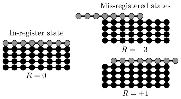
High resolution structures of amyloid fibrils show β-sheets composed of molecules perfectly aligned in the in-register state (left). However, fibrils grown at very high concentrations or grown from molecules with poor templating specificity can contain alignment defects (right). We describe the alignment between an incoming molecule (grey) and the existing fibril (black) using the registry variable R.
To indicate the alignment between an incoming molecule and the fibril end, we define the registry variable R, which can take the values −L < R < L, where L is the number of amino acids in each molecule (see Figure 1). Positive values of R indicate that the incoming molecule is shifted toward the C-terminus of the fibril template, while negative values denote a shift toward the N-terminus. R = 0 indicates a perfect alignment between the incoming molecule and the fibril. This will usually be the most stable state because it can form the most bonds. In the following, we compute the binding and unbinding times for simple sequences as a function of R. We use these calculations to show how amino acid sequences affect aggregation rates and assembly fidelity.
Theoretical Methods
Attachment rates
The on-rates can be related to the solution concentration using the Smoluchowski formula for particle striking an absorbing sphere
| (1) |
where a is the radius of the target (in this case, the fibril end) and D is the diffusion constant of the protein monomers. This expression for the attachment rate neglects several complications that my affect ron. These include the presence of states in the encounter complex that lack H-bonds, sidechain mediated bias in the registry selection, and free energy barriers in the initial binding. However, the overall growth rate is dominated by the registry lifetimes, making it unlikely that these effects will be more than a perturbation.21 In the remainder of this paper, we refer to the on-rate ron rather than the concentration, which is the more experimentally accessible quantity. While Eq. (1) provides a means to convert between these quantities, the effects above imply that this conversion is only approximate.
Binding lifetimes in the zipper model (1D reaction coordinate)
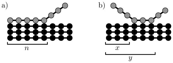
We are interested in the residence times of molecules that bind to the end of the fibril. We define tR(n) as the lifetime of a molecule that is bound to the fibril by n intermolecular H-bonds in registry R. We are particularly interested in tR(1), which is the average time that a molecule resides at the fibril end after making the first contact. We start with a simple model in which the bonds breakage starts at one end of the sequence and proceeds in a zipper-like manner toward the other end (see Figure 2).
Figure 2.
Cartoon of the two H-bonding models used in the calculations. a) The zipper model has a single reaction coordinate n that describes the number of H-bonds formed. Bonding begins on the left and progresses toward the right. The molecule unbinds when n = 0. b) In the two-dimensional model bonds can be broken at either end of the chain. A configuration is described using two reaction coordinates; x is the number of broken H-bonds on the left, and y is the position of the last formed H-bond on the right. The molecule unbinds when x = y and the fully bound state is when x = 0, y = L.
To begin, we define pR(n, t − t0) as the probability that a molecule that has n bonds at time t0 has neither broken or formed any bonds at time t. This probability obeys the equation
| (2) |
where r+(n + 1) is the formation rate of the (n + 1)th bond and r−(n) is the breakage rate of the nth bond. This equation has the trivial solution PR(n,t) = e−t/τR(n), where
| (3) |
is the average lifetime of state n.
Next, we write down a recursion relationship for the binding lifetimes27
| (4) |
This relationship says that the system will proceed from state n to state n + 1 with probability τR(n)r+(n + 1) and to state n − 1 with probability τR(n)r−(n). The final term accounts for the fact that the new random walks starting at these sites will begin after an average waiting time of τR(n) in state n.
To proceed from here we need to specify the bond formation and breakage rates. We assume that the formation rates are limited by the diffusion of the free polymer tails in solution and, therefore, are insensitive to the bonding energies.21 Therefore, we set r+ ≃ 1 ns.28 For the breakage rates, we assume an Arrhenius dependence on the binding energy, which gives r− = r+e−ε0.20
Here we demonstrate how transfer matrices can be used to solve Eq. (4) for a sequence with uniform binding energies. In the Supporting Information, we extend this formalism to solve for the binding lifetimes of triblock and alternating sequences.
When all bonds have the same binding affinity, the position arguments can be dropped from the bond breakage and formation rate constants, along with the R subscripts. The recursion relation (Eq. (4)) can be reduced to a homogenous form using the substitution
| (5) |
which yields
| (6) |
Eq. (6) can be re-written in the matrix form u(n + 1) = Mu(n) where
| (7) |
| (8) |
The matrix can be brought into diagonal form with the the transformation
| (9) |
| (10) |
By repeatedly applying the transfer matrix we can generate the u vector for any number of bonds
| (11) |
| (12) |
| (13) |
where we have used the boundary condition θ(0) = 0. The second boundary condition follows from the requirement that r+(L) = 0, which can be plugged into Eq. (4) to yield t(L) = t(L −1) + 1/r−(L). Inserting the vector components of Eq. (6), with Eq. (5), into the second boundary condition allows us to solve for the unknown constant
| (14) |
The residence time after the formation of the first bond is obtained by undoing the transformation from t to θ (Eq. (5))
| (15) |
Binding from both ends of molecule (2D reaction coordinate)
While the zipper model described above can be readily solved for the binding lifetimes, it has the unrealistic feature that only one end of the peptide is allowed to fluctuate. To correct for this, albeit in a model that will require numerical treatment, we describe the state of the incoming molecule using two reaction coordinates. These coordinates are shown in Figure 2b; x is the number of unrealized H-bonds on the N-terminus of the fibril template, and y is the position of the last formed H-bond. Therefore, L − y is the number of broken H-bonds at the C-terminus. With these definitions, the condition x < y describes states where the molecule is attached to the fibril and x = y indicates that the molecule has become unbound.
Generalizing Eq. (4), the binding times are related by the recursion relationship
| (16) |
where r+N (x + 1) is the breakage rate of the (x + 1)th bond, r−N (x) is the formation rate of the xth bond, r+C(y + 1) is the formation rate of the (y + 1)th bond, and r−C(y) is the breakage rate of the yth bond. This equation reflects the fact that after time τ(x,y) = (r+N + r−N + r+C + r−C)−1 the system evolves to state (x + 1, y) with probability τ(x,y)r+N (x + 1), to state (x − 1, y) with probability τ(x,y)r−N (x), etc. We use the binding energies for a given sequence to determine the breakage rates r−N (x) = r+eε(x) and r+C(y + 1) = r+eε(y+1), where the site specific binding energies are obtained from Table 1 in.12 Next, the system of equations, Figure 2, along with the boundary conditions t(x,x) = 0, r−N (0) = r+C(L) = 0, are solved numerically using Mathematica.
The lifetime of a given registry is the time between the formation of the first bond and the final unbinding. This is given by
| (17) |
where the summation is an average over the possible locations for the first bond to form.
Results and Discussion
High protein concentration increases the probability that transiently bound molecules will be incorporated in the fibril
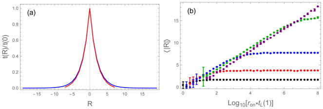
The large number of possible alignments between a soluble molecule and the fibril template results in a wide range of binding lifetimes. Figure 3a plots the binding state lifetimes of a homopolymer as a function of the alignment R as calculated from Eq. (15). In agreement with the simple Arrhenius argument above, the lifetimes decline exponentially as R deviates from the perfectly aligned state R = 0.
Figure 3.
(left) Bound state lifetimes (computed from Eq. (6) and Eq. (14)) as a function of the alignment between the incoming molecule and the fibril. The lifetime is maximized in the perfectly aligned state (R = 0) and drops exponentially as |R| increases. (right) Capture probabilities (Eq. (18)) of the uniform sequence as a function of the alignment. As the concentration increases, the rate of monomer collisions with the fibril end increases from ron=104 s−1 (black), 106 s−1 (red), to 108 s−1 (blue). The capture probability transitions from a sharply peaked function at R = 0 to a broad plateau. The plateau indicates that many mis-registered molecules are incorporated in the fibril. ε0 = 0.5, L = 20
The net growth of the fibril is determined by comparing these off-rates to the diffusion limited attachment rate ron. To make the comparison between the on- and off-rates in a simple way, we introduce the probabilities P±(R). We use the reciprocal of tR(1) as the off-rate of a molecule bound in state R, roff(R) = 1/tR(1). P+(R) gives the probability that a molecule bound in registry R remains attached to the fibril end long enough for the next molecule to bind
| (18) |
while
| (19) |
is the probability that a newly bound molecule detaches before the next binding event. P+ gives an estimate of the probability that a newly bound molecule will be incorporated in the fibril (the approximation comes from the fact that subsequent unbinding events can re-expose a buried molecule giving it another opportunity to unbind). Figure 3b shows P+(R) for several values of the concentration. For small values of c the capture probability can be approximated P+ ≃ ron/roff, which has a shape similar to the lifetimes plotted in Figure 3a, however, at higher concentrations the central peak becomes broader and eventually forms a wide plateau. This indicates that at these higher concentrations the assembly process becomes less selective and molecules with higher degrees of mis-alignment become incorporated in the fibril.
For our investigation of sequence effects we consider sequence motifs for which we can obtain analytic expressions for the binding lifetimes. To simplify the analytic treatment, we consider a reduced sequence space consisting of two types of amino acids. Following the work of Dill and coworkers,29,30 we label the two types as H (hydrophobic) and P (polar). Interactions between two H residues result in a strong binding energy εs = ε0 + |δ| while H-P and P-P interactions result in a weak binding energy εw = ε0 − |δ|. The corresponding bond breakage rates are r− = r+e−εs for H-H bonds and r− = r+e−εw for H-P and P-P bonds. The sequences are shown in Figure 4. There are two chains of alternating amino acids (HP)L/2 and (PH)L/2 that we denote ALT+ and ALT−, respectively. Next, there are two triblock copolymers; PL/4-HL/2-PL/4, which we label HSC to indicate the central aggregation-prone hot spot, and HL/4-PL/2-HL/4, which we refer to as HSF due to the pair of aggregation-prone hot spots flanking the central region. ALT+ and ALT− (and, similarly, HSC and HSF) are mathematically identical, differing only in the sign of the binding energy perturbation δ. We use δ > 0 for the cases where the leftmost amino acid has a strong binding energy. Finally, we compare these motifs to a uniform sequence (UNI) of L amino acids that all bind with energy ε0.
Figure 4.
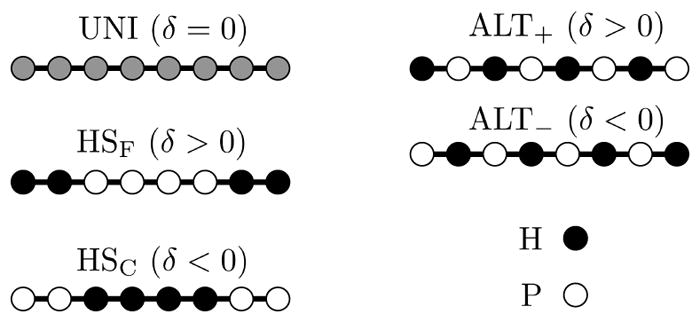
Cartoon representation of sequence motifs. UNI is a sequence where all amino acids have identical binding energies. ALT sequences alternate H and P residues. The subscript indicates the sign of the binding energy perturbation δ. Positive δ indicates that the sequence begins with a H residue so the first bond is strong. The remaining sequences are triblock polymers with an aggregation prone region either in the center (HSC) or split between the two flanking regions (HSF).
Binding lifetimes show Arrhenius scaling with sequence dependent perturbations
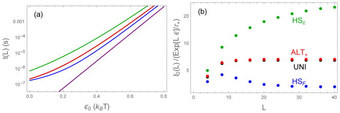
It is useful to examine the effect of sequence perturbations on the fully bound state t0(L) because the sequences have the same binding energy when all bonds are formed and the molecules are perfectly aligned (R = 0). Figure 5 shows the residence times for the simple sequences described above starting from the fully bound state, as calculated from Eq. (15) (UNI), S2, S11 (HS), S24, S25, and S30 (ALT). All sequences show Arrhenius scaling for large binding energies. However, the similarity on a logarithmic scale conceals the dramatic differences in residence times. To explore these differences there are two convenient limits to impose on the cumbersome expressions for the binding lifetimes. First, as seen in Figure 5b, for chain lengths greater than ~ 20 the sequence effects are confined to a constant factor that is multiplied by an Arrhenius term. These sequence dependent factors can be obtained by dividing the residence time by an Arrhenius rate factor
Figure 5.
Bound state lifetimes for sequences starting from the fully bound state. UNI (black), ALT+ (red), HSC (green), HSF (blue). (a) When the average binding energy ε0 exceeds ~ 0.5 the sequences follow an Arrhenius trend, although all sequences have lifetimes greater than the Arrhe-nius estimate (Eq. (20), purple). δ = 0.3, L = 20 (b) Ratio of binding lifetimes to the Arrhenius estimate (Eq. (20)) as a function of the sequence length. At large L the ratio becomes constant, indicating Arrhenius scaling. With these parameters (ε0 = 0.5, δ = 0.3) UNI and ALT sequences nearly superimpose.
| (20) |
and taking the large L limit. We obtain
| (21) |
| (22) |
| (23) |
where the final expression is valid for both central and flanking hot spots provided that −|ε0| < δ < 3ε0. Eq. (21)–Eq. (23) result in the ranking of retention times: HSC > ALT+ > UNI > ALT− > HSF (Figure 5b). To understand this ranking, it is useful to explore the second limit, that of small δ. In this limit the retention times are
| (24) |
for the triblock sequences, where δ > 0 corresponds to HSF and δ < 0 gives the result for HSC. The corresponding expression for the alternating sequence is
| (25) |
where δ > 0 gives ALT+ and δ < 0 gives ALT−. In both expressions the first term gives the binding time of UNI. Of greater interest is the first order term. In particular, the HS first order term is always negative and has a greater magnitude than the ALT first order term. These first order perturbations give rise to the ranking listed above (Figure 6a).
Figure 6.
Binding lifetimes as a function of the energy perturbation parameter δ starting from the fully bound state (a) and from the initial contact state (b). The two plots differ primarily in the vertical scale. This is because the initial contact lifetime is an average of event where the molecules proceed to the fully bound state and events where the molecules unbind almost immediately (on the nanosecond timescale). These averages are dominated by the fully bound states. For large values of |δ| all four sequences have lifetimes that are increasing function of |δ| because the weakly bound sites are net repulsive and contribute minimally to the binding lifetime. ε0 = 0.5, L = 20
Figure 6 also shows the residence times for large values of δ that lie outside the linear regime described by Eq. (24)–Eq. (27). For sufficiently large values of δ the residence times increase sharply, particularly for the triblock sequences. In these strongly asymmetric systems, the weakly bound sites are net repulsive, so the strongly bound sites dominate the unbinding rate.
The average binding lifetime is dominated by events where the molecule forms all possible bonds
A more relevant quantity for fibril growth is the residence time after only the first bond is formed. The leading order expressions for the first contact lifetimes are
| (26) |
for the triblock sequences. The corresponding expression for the alternating sequence is
| (27) |
Interestingly, even with only a single bond formed, it is more beneficial to have a long continuous string of strongly binding amino acids than it is to have a smaller number of strong sites near the initial binding site (Figure 6b). This is because, to a first approximation, this binding lifetime is an average of two outcomes. For binding energies on the order of kBT, the molecule will unbind before forming additional bonds roughly half of the time.20 However, once additional bonds start forming, it becomes overwhelmingly likely that it will proceed to the fully bound state. Accordingly, we observe the same ranking of lifetimes observed from the fully bound state. From Eq. (26) we can see that the superiority of HSC over HSF holds as long as ε0 is attractive.
Binding lifetime trends are independent of initial contact site
An unrealistic assumption of our zipper-like binding mechanism is that the first binding site is always weak for HSC and strong for HSF. In reality, the first contact between molecules can occur anywhere along the sequence. To investigate the effect of the point of initial contact, we looked at a model in which the H-bonds can initiate at any point along the sequence and form/break independently at both ends of the chain. If we require that the H-bonds are grouped in one continuous stretch, the problem reduces to a two-dimensional random walk where the two reaction coordinates are the number of broken H-bonds at the left and right ends of the chain.
Figure 7 plots the binding lifetimes for both triblock sequences as a function of the initial contact sites. Grouping the aggregation prone residues in a single hot spot has a dramatic effect on the binding lifetimes. In fact, the shortest lifetimes computed for HSC, which occur when the first contact is at a weak binding site at the edge of the sequence, is comparable to the longest lifetime of HSF, which occurs for a first contact in the middle of one of the hot spots. We also computed the lifetimes of a 10-10 diblock polymer and a 5-5-5-5 tetrablock. These sequences support the conclusion that having a contiguous stretch of strongly binding residues is more important than the binding affinity at the first contact.
Figure 7.
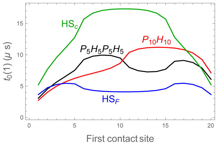
Binding lifetimes as a function of the location of the first contact for diblock, triblock, and tetrablock sequences. For all sequences there is a noticeable increase in the lifetime when the first contact is a strong binding site. This is due to the reduced probability of rapid dissociation. ε0 = 0.5, δ = 0.2
Adding weakly binding residues increases the number of trajectories that lead to unbinding
The strong reduction in the binding time of the diblock sequence relative to HSC (Figure 7) suggests that HSC may derive its strength from the weak flanking regions that protect the hot spot from the rapid bond fluctuations that occur at the polymer ends. This hypothesis can be rejected by computing the binding lifetimes for a diblock sequence in the one-dimensional model. This calculation yields an even function of δ, which says that breaking a strong region followed by a weak region has exactly the same binding time as breaking them in the opposite order (data not shown). Thus, a weak region has no protective effect on the unbinding of a strong region.
The explanation for the strength of the HSC motif can be deduced by considering the limit of highly asymmetric binding energies εw = 0, εs ≫ 1. In this case, left and right moves within the weakly bound regions will have equal probability, leading to a highly degenerate set of diffusive trajectories. In contrast, within the strongly bound regions, the probability of breaking a bond is very small e−εs ≪ 1. Therefore, the rupturing of hot spots is dominated by ballistic trajectories because each backward step that is added to a trajectory suppresses the probability by an additional factor of e−εs.
This simple argument show that there is a deleterious effect on the binding lifetimes from clustering weakly binding residues, just as there is a benefit from clustering strong ones. This is because groups of weak binding residues increase the multiplicity of trajectories that lead to unbinding. Of course, when dealing with a fixed number of strong and weak residues, as in our model sequences, breaking up a hot spot by adding weak residues comes with the compensating effect of shortening a weakly bound region. This can be seen from the minor difference between the diblock and tetrablock sequences in Figure 7. The way to avoid this tradeoff is to divide either the strong or weak residues across the two ends of the sequence, which explains the dramatic difference between HSC and HSF.
Sequence heterogeneity enhances templating efficiency
As noted earlier, single amino acid registry mismatches are less probable, in equilibrium, than the perfectly aligned state. For a uniform sequence each amino acid of registry mismatch reduces the Boltzmann weight by eε0. This reduction can be much greater if the binding energy is localized to a binding hot spot. Consider the HSC sequence, which has most of the binding energy localized to the central H block. Here a registry shift of one amino acid ruptures a weak bond at the edge and also replaces a strong H-H bond in the hot spot with a weak H-P bond. This results in a total energy change of ε0 + δ. As another example, a single amino acid shift with the HSF sequence will break two H-H bonds and replace one of them with a weak bond for a total energy change of ε0 + 3δ. Larger energy penalties for alignment shifts can be achieved by separating the strongly binding residues into greater number of hot spots. The ALT sequences represent the extreme case where a single amino acid shift breaks all strong bonds. However, a shift of 2 amino acids brings the H residues back into alignment allowing all but one of them to reform.
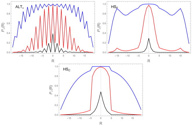
The alignment specificity can be seen by looking at the capture probabilities (Eq. (18)) for the HP sequences (Figure 8). The ALT sequence shows a striking even/odd effect reflecting the fact that odd registries only permit the formation of weak H-P bonds, while even registries contain equal numbers of strong and weak bonds. However, viewed separately, the even and odd registries each show the same exponential dependence seen in Figure 3. The triblock sequences show sharper central peaks than UNI (Figure 3b) as a result of the greater energy penalty for mis-alignment described above. HSF also shows secondary peaks where the C-terminal hot spot of one molecule aligns with the N-terminal hot spot of the adjacent molecule.
Figure 8.
Capture probabilities (Eq. (18)) as a function of binding alignment R and the diffusion collision rate ron=104 s−1 (black), 106 s−1 (red), to 108 s−1 (blue). Higher values of ron, corresponding to higher monomer concentration, result in greater probability for mis-registered molecules to be incorporated in the fibril. The HP sequences show considerably more structure than the exponential dependence of the UNI sequence (Figure 3) due to the effects of aligning the strong binding H residues. In particular, the ALT sequence has lower capture probabilities when R is odd because these alignments only allow for the formation of weak H-P bonds. Also, the HSF sequence shows secondary peaks at large |R| when the H residues from opposite ends of the chain are brought together. ε0 = 0.5, δ = 0.3
Fibril growth is the result of binding and unbinding events in all registries
An approximate expression for the growth rate can be obtained by assuming that only two outcomes are possible after a molecular attachment event; the molecule unbinds before the next attachment event, or it becomes permanently locked onto the fibril by the next binding event. The probabilities of the latter event are given by Eq. (18), which can be summed to give the growth rate
| (28) |
where the prefactor is the diffusion-limited attachment rate for each registry. Similarly, we can compute the average registry of the bound molecules
| (29) |
These approximate expressions assume that diffusion leads to the binding of all registries with equal probability. There are two shortcomings to Eq. (28) and Eq. (29). First, they do not have memory of previous binding events. That is, the unbinding of a molecule does not allow the previous molecule another chance to detach. Secondly, the computed growth rate is positive for all concentrations and, therefore, Eq. (28) cannot describe the dissolution of fibrils at concentrations below the solubility concentration. To account for these errors, we have performed Gillespie simulations of the growth process.31
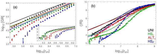
The fibril growth rate and average registry errors are shown in Figure 9. Eq. (28) and Eq. (29) agree well with the simulations at high growth rates, but show discrepancies at low concentrations. This is expected because multiple unbinding events, which are not accounted for in Eq. (28) and Eq. (29), will be common at low concentration but rare at high concentration. Interestingly, the analytic approximations do a good job of qualitatively capturing changes in the rank ordering of sequences, even at low concentration.
Figure 9.
Comparison of the fibril growth rate and average registry computed by Eq. (28) and Eq. (29) (lines) and Gillespie simulation (dots). (a) Growth rate (molecules per second) as a function of the diffusion-limited binding rate. The theory, while quantitatively inaccurate, correctly predicts changes in the ranking of sequences as a function of concentration. (inset) The low concentration regime shows a sharp increase in the growth rate at the solubility concentration. (b) The theory also does a good job of predicting the relative order of average registries, even at low concentration. The HSF has the most ordered fibrils at low concentration (small ron), but becomes less ordered than the other sequences at high concentration when large registry mismatches become more common. These large mismatches promote binding events between H residues at opposite ends of the triblock. Error bars show the standard deviation from three simulations. ε0 = 0.5, δ = 0.3
Sequences with poor templating efficiency grow fastest
The uniform sequence has the highest growth rates over all concentrations studied (Figure 9a). This increased growth rate is due to off-register states; the uniform sequence has the highest affinity for off-register states, so these states are more readily incorporated in the fibril. Therefore, the uniform sequence also has the highest average registry error (Figure 9b).
Neglecting the highly disordered UNI sequence, the ranking of growth rates and solubility concentrations follows the ranking of residence times discussed above, because longer residence times promote faster growth. The influence of the disordered states has a more complicated effect on the fibril order parameter 〈|R|〉. Interestingly, the best sequence for growing ordered fibrils depends on the monomer concentration in the solution. At low concentrations we expect that the distribution of registries is dominated by small errors. From Figure 8 we see that HSF is the most effective sequence for rejecting small registry errors and, therefore, it results in the most highly ordered fibrils at low concentrations (Figure 9b). However, at higher concentration large registry mismatches come into play. Here HSF is particularly prone to large errors due to the secondary peaks in its capture probability (Figure 8). Because of this, HSF transitions from being the most ordered at low concentration to the most disordered at high concentration.
Small registry errors occur with similar probability for short and long sequences
The incidence of registry errors does not depend strongly on the chain length. Figure 10a shows that the residence times for small mismatches scales with the same Arrhenius dependence for both short (L = 8) and long (L = 20) chains. Therefore, these small mismatches should be incorporated at similar rates, provided the solutions are prepared with similar supersaturation. This is confirmed in Figure 10b which shows 〈|R|〉 as a function of concentration for uniform sequences of varying length. In all cases we observe that 〈|R|〉 ∝ ln c until the increase saturates at 〈|R|〉 ≃ L/2 at high concentration, indicating a completely random distribution of registries.
Figure 10.
Longer sequences can be used to grow more highly ordered fibrils. (a) Binding lifetimes decay exponentially for UNI chains regardless of the chain length. The lifetimes of L = 20 (blue) and L = 8 (red) chains superimpose when scaled by the lifetime of the in-register state. This means that registry mismatches at the same R will be incorporated at similar rates for both systems when the fibrils are grown near their solubility concentration. (b) The average alignment error increases proportional to ln ron (or ln c). The curves collapse to a single line when the diffusion rates are scaled by the lifetime of the in-register state. This is because the in-register lifetime scales with the reciprocal of the solubility concentration. Since chains of different length have similar 〈|R|〉 at the same supersaturation, the relative mismatch, 〈|R|〉/L can be minimized with longer chains. ε0 = 0.5
The transition from ordered to disordered aggregates shown in Figure 9b and Figure 10b is very slow, requiring concentration increases of many orders of magnitude. This transition can be achieved more rapidly by changing solvent conditions. For example, if the molecules are charged, changing the salt concentration or pH of the solution has the compound effect of simultaneously increasing ron by reducing the electrostatic diffusion barrier, and increasing the lifetime of molecules bound to the fibril.
The exponential suppression of registry errors shown in Figure 10a explains the high degree of order seen in Huntingtin aggregates. NMR measurements have shown that approximately 25% of molecules in Huntingtin fibrils show registry shifts.32 Although the interpretation of these experiments is complicated by the effects of flanking non-amyloidogenic sequences, a binding energy on the order of 1–1.5 kBT is probably sufficient to suppress registry errors to this level.
Sequences of natural amino acids are efficient at preventing registry errors
Next, we apply our model to sequences of the 20 natural amino acids. This greatly increases the complexity of the system since there will be 400 energy parameters in the model instead of the two parameters in our HP model. While these energy parameters can be extracted from simulations, this has only been done for a small number of amino acid pairs.21 As an imperfect replacement for these energies, we employ the pairwise aggregation propensities determined by Trovato et al.12 These parameters are obtained from a bioinformatic approach, but they have magnitudes comparable to the free energies of binding and should capture which interactions are favorable and which are unfavorable. However, the lifetimes we calculate from these “energies” are not quantitative. Therefore we restrict ourselves to qualitative conclusions only.
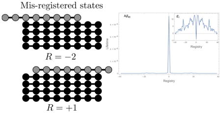
Figure 11 plots the residence times for Aβ and IAPP as a function of the registry R. These residence times are calculated from the two-dimensional diffusion model (Figure 2) that allows for bond breakage at both ends of the chain. The lifetimes of each registry are averaged over the L −|R| initial contact points. It is striking that the lifetimes are much more sharply peaked at R = 0 than those of the HP sequences (see Figure 3b and Figure 8). In fact, the ratio of the lifetime for the in-register state to the lifetime of the single amino shift (R = ±1) is on the order of 102. This means that, unlike the HP sequences, natural sequences will be able to achieve highly ordered fibrils, with 〈|R|〉 close to zero over a range of concentrations. Furthermore, the similarity in the binding lifetimes of the mis-registered states suggests that these sequences will transition more abruptly from ordered fibrils to disordered aggregates.
Figure 11.
Binding lifetimes of Aβ40 and IAPP as a function of alignment. In both cases the lifetime of the in-register state is two orders of magnitude greater than any other state. This separation of timescales allows for the growth of highly ordered fibrils. (inset) Binding energy EI as a function of alignment. The in-register state is a deep well at R = 0. The high energy of the R = ±1 states prevents the incorporation of these “near misses” in the fibril.
To explore the cause of this templating efficiency, we translated the Aβ and IAPP sequences to the HP model using the Kyte-Doolittle scale with a cutoff between tryptophan and serine.33 We varied εs from 0.7 to 1.3 kBT while scaling εw to satisfy the requirement that the binding energy of Aβ residues 12–40 summed to 15 kBT.34 All parameter sets reproduced the main features of the binding lifetimes shown in Figure 11, with a central peak two orders of magnitude higher than the mis-registered states. This suggests that templating efficiency arises from having hot spots of varying length and separation. This minimal complexity, which arises naturally from the enrichment of hydrophobic amino acids in Aβ, is sufficient to produce a large energy penalty for registry errors while retaining the binding affinity of hydrophobic hot spots. In contrast, randomly generated sequences do not contain these hydrophobic stretches, due to the equal proportion of hydrophobic and polar residues, and are predicted by both the HP and 20 amino acid models to have negligible binding (data not shown).
Binding free energies have an inverted funnel topology
The insets to Figure 11 show the bioinformatic binding energies EI as a function of the molecular alignment. As expected, there is a deep well at R = 0 corresponding to the in-register state. Conversely, the R = ±1 states have very high energy. In both molecules there are some registries that have energies approaching the R = 0 state, but these highly mis-aligned states form few H-bonds so the calculated residence times are much shorter than the in-register state.
The overall shape of the energy landscape is remarkable in that there is no bias toward the in-register state. In order for proteins to fold into a native state in physiological timescales, it is necessary to have an energetic bias, often depicted as a funnel, that guides the folding process.35 The energy landscapes in the insets of Figure 11 do not have this feature and, instead, resemble a “golf course” or even an inverted funnel landscape.35,36 Amyloid fibrils are able to form without the aid of an energetic bias because the simple cross-β structure has a much smaller state space, described by our R variable, than the vast combinatorics of backbone dihedral angles in protein folding. An important consequence of this unbiased landscape is that aggregation occurs by a random search over configuration space that is not dominated by a small number of trajectories or intermediate states. As a result, it is difficult to predict or explain the effects of mutations because the net effect is an accumulation of small perturbations over the entire “non-native” ensemble.21
Shuffled sequence variants show the same clustering trends as the HP model
We can be somewhat more quantitative in our analysis by examining sequences with the same amino acid composition but different ordering. Since these sequences all have the same binding energy, the only difference in the residence time arises from the position of amino acids within the sequence. Monsellier et al. constructed four scrambled variants of apomyoglobin (apoMb1–29) and measured their aggregation rates along with the wild type.37 Figure 12 compares the measured aggregation rates to the elongation rates calculated from Eq. (28). While the theoretical rates are not directly comparable to the experimental rates due to the non-physical energy parameters and complications like nucleation, our theory does a good job of ranking the aggregation propensity of the sequences, getting 4 out of 5 sequences correct.
Figure 12.
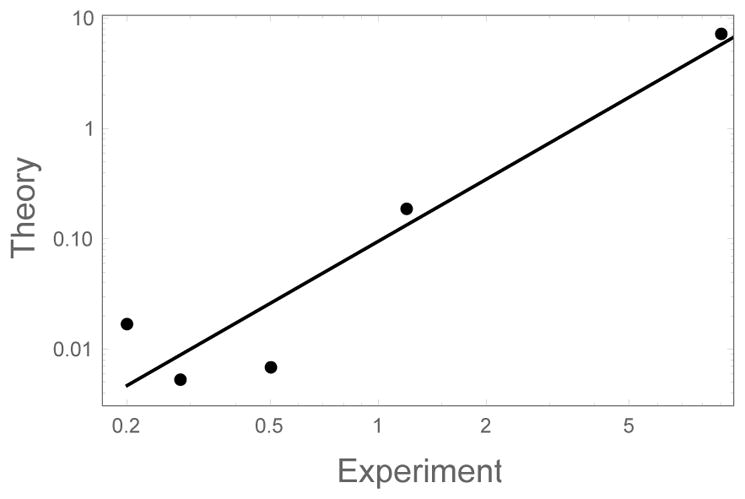
Comparison of the computed growth rates of apoMb derived sequences to the growth rates measured by circular dichroism.37 The units of the theoretical calculation cannot be determined due to our use of energy parameters derived from bioinformatics. Calculations performed using ron = 103 s−1. Similar results are obtained for other values of the diffusion rate (i.e. monomer concentration) or for other experimental assays of the growth rate.
An inspection of the modified sequences reveals the mechanism of aggregation enhancement. Monsellier et al. found that the aggregation propensity is highly correlated with the width of the most aggregation prone region. They were able to increase the width of the hot spot by moving aggregation prone residues from the periphery of the sequence to the middle.37 The analog of these manipulations in our HP model would be to modify the ALT sequence to resemble HSC. Therefore, the correlation observed by Monsellier et al. can be explained by the long residence times of HSC in our HP model. We note that, in addition to promoting fibril elongation, clustering the aggregation prone residues into a single hot spot will be highly beneficial to surmounting the entropic barrier associated with fibril nucleation.38,39
Conclusion
While the amyloid state is a generic property of the polypeptide backbone,7,8 the sequence of side chains clearly matters. Our simple model shows that sequences with identical binding energies can have widely varying binding lifetimes depending on the arrangement of amino acids.
The growth rate of a fibril depends on both the attachment rate of new molecules and the rate molecules detach. Highly ordered fibrils are grown when molecules bound in-register are retained on the fibril while mis-aligned molecules unbind faster than new molecules can arrive. Sequences like Aβ and IAPP contain hot spots of varying length and separation, providing a lock-and-key fit that provides strong discrimination between in-register and mis-aligned states. In contrast, molecules like Huntingtin and low complexity domains in biomaterials display repetitive motifs that allow for more heterogeneity in binding.6 In these latter cases there may be a tradeoff between the strength conferred by high fidelity binding and the rapid self-healing afforded by promiscuous binding.
Detailed calculations of the alternating and triblock sequence binding lifetimes are available in the Supporting Information.
Supplementary Material
Acknowledgments
This work was supported by NIH Grant R01GM107487 and the REU program funded by the National Science Foundation (NSF) and the Air Force Office of Scientific Research (AFOSR) through NSF grant number PHYS-1461251. We would like to thank the referee for suggesting the HP analysis of Aβ and IAPP.
References
- 1.Anfinsen CB. Principles that Govern the Folding of Protein Chains. Science. 1973;181:223–230. doi: 10.1126/science.181.4096.223. [DOI] [PubMed] [Google Scholar]
- 2.Baldwin AJ, Knowles TPJ, Tartaglia GG, Fitzpatrick AW, Devlin GL, Shammas SL, Waudby CA, Mossuto MF, Meehan S, Gras SL, et al. Metastability of Native Proteins and the Phenomenon of Amyloid Formation. J Am Chem Soc. 2011;133:14160–3. doi: 10.1021/ja2017703. [DOI] [PubMed] [Google Scholar]
- 3.Tycko R, Wickner RB. Molecular Structures of Amyloid and Prion Fibrils: Consensus Versus Controversy. Acc Chem Res. 2013;46:1487–1496. doi: 10.1021/ar300282r. [DOI] [PMC free article] [PubMed] [Google Scholar]
- 4.Knowles TPJ, Vendruscolo M, Dobson CM. The Amyloid State and its Association with Protein Misfolding Diseases. Nat Rev Mol Cell Biol. 2014;15:384–96. doi: 10.1038/nrm3810. [DOI] [PubMed] [Google Scholar]
- 5.Fowler DM, Koulov AV, Balch WE, Kelly JW. Functional Amyloid - From Bacteria to Humans. Trends Biochem Sci. 2007;32:217–224. doi: 10.1016/j.tibs.2007.03.003. [DOI] [PubMed] [Google Scholar]
- 6.So CR, Fears KP, Leary DH, Scancella JM, Wang Z, Liu JL, Orihuela B, Rittschof D, Spillmann CM, Wahl KJ. Sequence Basis of Barnacle Cement Nanostructure is Defined by Proteins with Silk Homology. Sci Rep. 2016;6:36219. doi: 10.1038/srep36219. [DOI] [PMC free article] [PubMed] [Google Scholar]
- 7.Guijarro J, Sunde M, Jones J, Campbell I, Dobson CM. Amyloid Fibril Formation by an SH3 Domain. Proc Natl Acad Sci U S A. 1998;95:4224–4228. doi: 10.1073/pnas.95.8.4224. [DOI] [PMC free article] [PubMed] [Google Scholar]
- 8.Dobson CM. Protein Folding and Misfolding. Nature. 2003;426:884–90. doi: 10.1038/nature02261. [DOI] [PubMed] [Google Scholar]
- 9.Caflisch A. Computational Models for the Prediction of Polypeptide Aggregation Propensity. Curr Opin Chem Biol. 2006;10:437–44. doi: 10.1016/j.cbpa.2006.07.009. [DOI] [PubMed] [Google Scholar]
- 10.Fernandez-Escamilla AM, Rousseau F, Schymkowitz J, Serrano L. Prediction of Sequence-Dependent and Mutational Effects on the Aggregation of Peptides and Proteins. Nat Biotechnol. 2004;22:1302–6. doi: 10.1038/nbt1012. [DOI] [PubMed] [Google Scholar]
- 11.Conchillo-Solé O, de Groot NS, Avilés FX, Vendrell J, Daura X, Ventura S. AG-GRESCAN: A Server for the Prediction and Evaluation of “Hot Spots” of Aggregation in Polypeptides. BMC Bioinf. 2007;8:65. doi: 10.1186/1471-2105-8-65. [DOI] [PMC free article] [PubMed] [Google Scholar]
- 12.Trovato A, Chiti F, Maritan A, Seno F. Insight Into the Structure of Amyloid Fibrils from the Analysis of Globular Proteins. PLoS Comput Biol. 2006;2:e170. doi: 10.1371/journal.pcbi.0020170. [DOI] [PMC free article] [PubMed] [Google Scholar]
- 13.Tartaglia GG, Vendruscolo M. The Zyggregator Method for Predicting Protein Aggregation Propensities. Chem Soc Rev. 2008;37:1395. doi: 10.1039/b706784b. [DOI] [PubMed] [Google Scholar]
- 14.Maurer-Stroh S, Debulpaep M, Kuemmerer N, de la Paz ML, Martins IC, Reumers J, Morris KL, Copland A, Serpell L, Serrano L, et al. Exploring the Sequence Determinants of Amyloid Structure Using Position-Specific Scoring Matrices. Nat Meth. 2010;7:237–242. doi: 10.1038/nmeth.1432. [DOI] [PubMed] [Google Scholar]
- 15.Pawar AP, Dubay KF, Zurdo J, Chiti F, Vendruscolo M, Dobson CM. Prediction of “Aggregation-Prone” and “Aggregation-Susceptible” Regions in Proteins Associated with Neurodegenerative Diseases. J Mol Biol. 2005;350:379–92. doi: 10.1016/j.jmb.2005.04.016. [DOI] [PubMed] [Google Scholar]
- 16.Galzitskaya OV, Garbuzynskiy SO, Lobanov MY. Expected Packing Density Allows Prediction of Both Amyloidogenic and Disordered Regions in Protein Chains. J Phys Cond Mat. 2007;19:285225. [Google Scholar]
- 17.Garbuzynskiy SO, Lobanov MY, Galzitskaya OV. Fold Amyloid: A Method of Prediction of Amyloidogenic Regions From Protein Sequence. Bioinformatics. 2010;26:326–332. doi: 10.1093/bioinformatics/btp691. [DOI] [PubMed] [Google Scholar]
- 18.Tian J, Wu N, Guo J, Fan Y. Prediction of Amyloid Fibril-Forming Segments Based on a Support Vector Machine. BMC Bioinf. 2009;10:S45. doi: 10.1186/1471-2105-10-S1-S45. [DOI] [PMC free article] [PubMed] [Google Scholar]
- 19.Lee CF, Loken J, Jean L, Vaux DJ. Elongation Dynamics of Amyloid Fibrils: A Rugged Energy Landscape Picture. Phys Rev E. 2009;80:041906. doi: 10.1103/PhysRevE.80.041906. [DOI] [PubMed] [Google Scholar]
- 20.Schmit JD. Kinetic Theory of Amyloid Fibril Templating. J Chem Phys. 2013;138:185102. doi: 10.1063/1.4803658. [DOI] [PubMed] [Google Scholar]
- 21.Jia Z, Beugelsdijk A, Chen J, Schmit JD. The Levinthal Problem in Amyloid Aggregation: Sampling of a Flat Reaction Space. J Phys Chem B. 2017;121:1576–1586. doi: 10.1021/acs.jpcb.7b00253. [DOI] [PMC free article] [PubMed] [Google Scholar]
- 22.Schmit JD, Dill KA. Growth Rates of Protein Crystals. Journal of the American Chemical Society. 2012;134:3934–7. doi: 10.1021/ja207336r. [DOI] [PMC free article] [PubMed] [Google Scholar]
- 23.Whitelam S, Dahal YR, Schmit JD. Minimal Physical Requirements for Crystal Growth Self-Poisoning. J Chem Phys. 2016;144:064903. doi: 10.1063/1.4941457. [DOI] [PMC free article] [PubMed] [Google Scholar]
- 24.Becher MW, Kotzuk JA, Sharp AH, Davies SW, Bates GP, Price DL, Ross CA. Intranuclear Neuronal Inclusions in Huntington’s Disease and Dentatorubral and Pallidoluysian Atrophy: Correlation Between the Density of Inclusions and IT15CAG Triplet Repeat Length. Neurobiol Dis. 1998;4:387–397. doi: 10.1006/nbdi.1998.0168. [DOI] [PubMed] [Google Scholar]
- 25.Walters RH, Murphy RM. Examining Polyglutamine Peptide Length: A Connection Between Collapsed Conformations and Increased Aggregation. J Mol Biol. 2009;393:978–992. doi: 10.1016/j.jmb.2009.08.034. [DOI] [PMC free article] [PubMed] [Google Scholar]
- 26.Crick SL, Ruff KM, Garai K, Frieden C, Pappu RV. Unmasking the Roles of N- and C-Terminal Flanking Sequences from Exon 1 of Huntingtin as Modulators of Polyglutamine Aggregation. Proc Natl Acad Sci U S A. 2013;110:20075–80. doi: 10.1073/pnas.1320626110. [DOI] [PMC free article] [PubMed] [Google Scholar]
- 27.Redner S. A Guide to First-Passage Processes. Cambridge University Press; 2007. p. 328. [Google Scholar]
- 28.Muñoz V, Thompson PA, Hofrichter J, Eaton WA. Folding Dynamics and Mechanism of Beta-Hairpin Formation. Nature. 1997;390:196–9. doi: 10.1038/36626. [DOI] [PubMed] [Google Scholar]
- 29.Dill KA. Theory for the folding and stability of globular proteins. Biochemistry. 1985;24:1501–9. doi: 10.1021/bi00327a032. [DOI] [PubMed] [Google Scholar]
- 30.Dill KA, Bromberg S, Yue K, Fiebig KM, Yee DP, Thomas PD, Chan HS. Principles of Protein Folding–A Perspective from Simple Exact Models. Protein Sci. 1995;4:561–602. doi: 10.1002/pro.5560040401. [DOI] [PMC free article] [PubMed] [Google Scholar]
- 31.Gillespie DT. Exact stochastic simulation of coupled chemical reactions. J Phys Chem. 1977;81:2340–2361. [Google Scholar]
- 32.Hoop CL, Lin HK, Kar K, Hou Z, Poirier MA, Wetzel R, van der Wel PCA. Polyglutamine Amyloid Core Boundaries and Flanking Domain Dynamics in Hunt-ingtin Fragment Fibrils Determined by Solid-State Nuclear Magnetic Resonance. Biochemistry. 2014;53:6653–6666. doi: 10.1021/bi501010q. [DOI] [PMC free article] [PubMed] [Google Scholar]
- 33.Kyte J, Doolittle RF. A Simple Method for Displaying the Hydropathic Character of a Protein. J Mol Biol. 1982;157:105–132. doi: 10.1016/0022-2836(82)90515-0. [DOI] [PubMed] [Google Scholar]
- 34.Schmit JD, Ghosh K, Dill KA. What Drives Amyloid Molecules to Assemble into Oligomers and Fibrils? Biophys J. 2011;100:450–8. doi: 10.1016/j.bpj.2010.11.041. [DOI] [PMC free article] [PubMed] [Google Scholar]
- 35.Dill KA, Chan HS. From Levinthal to Pathways to Funnels. Nat Struct Biol. 1997;4:10–19. doi: 10.1038/nsb0197-10. [DOI] [PubMed] [Google Scholar]
- 36.Granata D, Baftizadeh F, Habchi J, Galvagnion C, De Simone A, Camilloni C, Laio A, Vendruscolo M. The Inverted Free Energy Landscape of an Intrinsically Disordered Peptide by Simulations and Experiments. Sci Rep. 2015;5:15449. doi: 10.1038/srep15449. [DOI] [PMC free article] [PubMed] [Google Scholar]
- 37.Monsellier E, Ramazzotti M, de Laureto PP, Tartaglia GG, Taddei N, Fontana A, Vendruscolo M, Chiti F. The Distribution of Residues in a Polypeptide Sequence is a Determinant of Aggregation Optimized by Evolution. Biophys J. 2007;93:4382–4391. doi: 10.1529/biophysj.107.111336. [DOI] [PMC free article] [PubMed] [Google Scholar]
- 38.Zhang L, Schmit JD. Pseudo-One-Dimensional Nucleation in Dilute Polymer Solutions. Phys Rev E. 2016;93:060401. doi: 10.1103/PhysRevE.93.060401. [DOI] [PMC free article] [PubMed] [Google Scholar]
- 39.Zhang L, Schmit JD. Theory of Amyloid Fibril Nucleation from Folded Proteins. Isr J Chem. 2017;57:738–749. doi: 10.1002/ijch.201600079. [DOI] [PMC free article] [PubMed] [Google Scholar]
Associated Data
This section collects any data citations, data availability statements, or supplementary materials included in this article.


