Transcriptional Dynamics of Hair-Bundle Morphogenesis Revealed with CellTrails

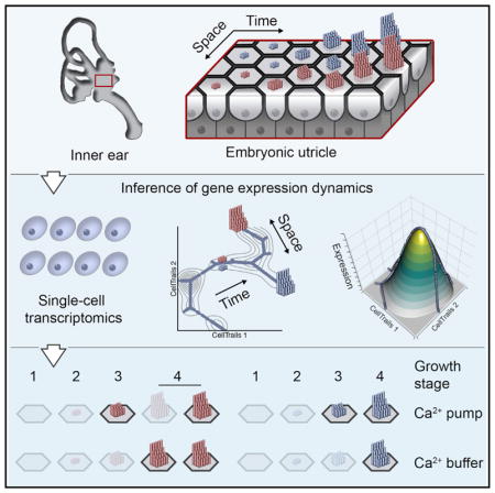
SUMMARY

Protruding from the apical surface of inner ear sensory cells, hair bundles carry out mechanotransduction. Bundle growth involves sequential and overlapping cellular processes, which are concealed within gene expression profiles of individual cells. To dissect such processes, we developed CellTrails, a tool for uncovering, analyzing, and visualizing single-cell gene-expression dynamics. Utilizing quantitative gene-expression data for key bundle proteins from single cells of the developing chick utricle, we reconstructed de novo a bifurcating trajectory that spanned from progenitor cells to mature striolar and extrastriolar hair cells. Extraction and alignment of developmental trails and association of pseudo-time with bundle length measurements linked expression dynamics of individual genes with bundle growth stages. Differential trail analysis revealed high-resolution dynamics of transcripts that control striolar and extrastriolar bundle development, including those that encode proteins that regulate [Ca²⁺]_i or mediate crosslinking and lengthening of actin filaments.

In Brief

Ordering single cells along branching trajectories using transcriptomic data is bioinformatically challenging. Ellwanger et al. developed CellTrails and applied this tool to showcase the bifurcating sequence of gene expression as sensory hair cells develop into different subtypes that feature spatially distinct morphologies of the mechanosensitive hair bundle.

INTRODUCTION

Hair bundles are the mechanosensitive organelles of sensory hair cells, which mediate the mechanical-to-electrical transduction that is at the heart of hearing and balance (Gillespie and Müller, 2009). The actin-filled stereocilia comprising a bundle are arranged in ranks of increasing height, producing an asymmetrical morphology that specifies the axis of physiological sensitivity—mechanotransduction channels open when a bundle is moved toward its tallest stereocilia and close when moved in the opposite direction (Fettiplace and Kim, 2014). Bundle structure therefore fundamentally underlies hair-cell function.

The morphological steps that occur during hair-bundle development (Tilney et al., 1992a) are evolutionarily conserved (Barr-Gillespie, 2015), yet underlying molecular changes are only sparsely known, mostly through identification of “deafness genes” (Barr-Gillespie, 2015; Drummond et al., 2012). Nevertheless, such identification is insufficient to catalog the proteins essential for bundle assembly, as some proteins may be essential for embryonic survival or are compensated for by a close paralog. Many of these additional proteins are likely present in mass-spectrometry analyses of the bundle’s proteome (Krey et al., 2015; Shin et al., 2013; Wilmarth et al., 2015). Inventorying molecules that participate in hair-bundle assembly is the first step toward developing a mechanistic understanding of this process (Pollard, 2014), and the available deafness gene and proteomics compilations provide the foundation to build upon.

The next step in characterizing hair-bundle development is to understand when each molecule is expressed by hair cells, as this sequence dictates the assembly process. Using single-cell analysis, we describe here the spatial and temporal expression of key hair-bundle transcripts. The full spectrum of developing and mature cell types exists in a single snapshot of an asynchronously developing organ, such as the chick utricle at embryonic day (E) 15 (Goodyear et al., 1999). In addition to developmental differences among cells, the utricle also shows regional variation in cell organization and structure, containing at least three types of hair cells (Figures 1A and 1B). The striola primarily contains type I hair cells, enveloped by afferent calyces, as well as a few striolar type II hair cells, which are centrally located at the line of hair-bundle polarity reversal and are contacted by synaptic boutons. Both striolar hair cell types display relatively short hair bundles with thick stereocilia; by contrast, extrastriolar type II hair cells—also contacted by synaptic boutons—have long hair bundles with thin stereocilia. Although type, location, and developmental age of individual cells are not preserved during single-cell sampling, we hypothesized that their transcriptional profiles encode this information. We therefore devised an algorithm, CellTrails, to determine the dynamically changing cellular states of a branching trajectory of utricle hair cells during bundle assembly. By using spectral decomposition of a robust cell-cell association index, CellTrails embeds the transcriptional profiles of cells into a low-dimensional representation—a manifold—that best characterizes the data. In situ hybridization and immunolabeling confirmed the predicted spatial information as well as transcription dynamics. Moreover, the precise temporal ordering of cells and accompanying expression changes in individual genes were robustly correlated with stereocilia elongation, which we utilized as an in situ ruler for developmental progression. CellTrails’ spatiotemporal mapping revealed gene-expression dynamics that specified unique stereocilia dimensions for striolar and extrastriolar hair cells and provided evidence for two distinct classes of extrastriolar type II hair cells.

Figure 1. Uncovering Spatiotemporal States of Bundle Development.

(A) Cytomorphological features of hair cells in medial and lateral extrastriolar (MES, LES) regions and in the striola. The line of polarity reversal (LPR) is indicated. We only show one example of striolar type II hair cells (bright orange), which are found on both sides of the LPR. The drawing was inspired by Jorgensen (1989).

(B) Top-down scanning electron microscopy (SEM) view of a medial-to-lateral stripe of the E15 chicken utricle; the enlarged inset shows the distinct hair-bundle shapes of cells in striolar and extrastriolar regions. A high-resolution version of the SEM data file is available at Mendeley Data (https://doi.org/10.17632/yy3c72972w.1).

(C) Isolation of cells from chicken utricles. 261 cells were sampled exclusively from either the lateral or the medial half. The fluorescence-activated cell sorting (FACS) plot shows the range of FM1–43 uptake. Rectangles delineate metadata labels; SSC-A, side scatter area.

(D) Lower-dimensional manifold learning. Fuzzy mutual information-based affinity scores were used to define edge weights of a complete graph with a cell at each node. Spectral decomposition of the graph was performed to unfold the manifold.

(E) Subspace dimensionality. Linear regression to the total eigengap values of the spectral embedding revealed nine relevant dimensions.

(F) Spectral clustering. The dendrogram displays the relationship between 25 clusters (leaf nodes) with at least 1% of cells in each. If the null hypothesis of a post hoc test on differential gene expression was accepted, siblings were iteratively merged, resulting in the 11 highlighted states.

(G) Spatiotemporal information. Bottom: the cell-to-cell distance matrix (L²-norm) in the low-dimensional space, which was used to compute initial clusters and their relationship (dendrogram). Top: the relative distribution of FM1–43-gated cells and cells with known spatial origin per determined state; *p < 10⁻³ by imputed Fisher test.

We further established a strategy for the alignment of extracted linear trajectories (trails), which allows comparison of gene expression dynamics as different hair-bundle types develop. Examining genes involved in hair-bundle development, which includes the processes of lengthening, widening, tapering, actin-crosslinking, transport, and transduction, we found that the Ca²⁺ regulators CALB2 (calretinin) and ATP2B2 (PMCA2) are dynamically regulated during stereocilia growth in different hair cell types. Precise spatiotemporal control of [Ca²⁺]_i consequently appears to be an important component of hair-bundle development.

Our analysis provides insight into spatial, temporal, and cytomorphological aspects of hair-bundle development at high resolution. Utilizing a concept of uncovering and visualizing latent spatiotemporal information from single-cell gene-expression data, CellTrails performs as well with RNA-seq data as it does with single-cell multiplex qRT-PCR data.

RESULTS

Transcriptional Profiling of Chicken Vestibular Cells

To determine gene expression patterns during hair-bundle development, we chose 183 genes associated with bundle structure, function, and development (Ku et al., 2014; Shin et al., 2013; Van Camp and Smith, 2017) (Table S1A). We obtained multiplex qRT-PCR transcriptional profiles of 1,008 single epithelial cells from chicken utricles at E15, when cells of all developmental stages are present (Goodyear et al., 1999) (Figure S1; Table S1B). We generated metadata by sampling cells either from the lateral region of the utricle (134 cells), which includes the striola, or from the medial extrastriolar (MES) side of the utricle (127 cells; Figure 1C). Further, we briefly exposed other utricles to FM1–43 and isolated 93 cells for which we recorded the level of uptake of the styryl dye; a high level of FM1–43 fluorescence is indicative of a functional mechanoelectrical transduction apparatus (Gale et al., 2001).

Spectral Embedding Reveals Latent Spatiotemporal Information

We hypothesized that the expression profiles of the 1,008 cells represent indirect measurements of underlying spatiotemporal features of each cell. By proper learning of a low-dimensional manifold, we expected to reveal this latent information and to reduce noise by removing irrelevant or highly correlated variables. We employed the geometrically motivated concept of nonlinear spectral embedding (Figure 1D) (Belkin and Niyogi, 2003; Sussman et al., 2012). Due to its locality-preserving character, this technique is advantageous because it is insensitive to outliers and noise, is not susceptible to short-circuiting, and emphasizes naturally occurring clusters in the data. The data’s manifold structure was represented by a simple graph connecting cells by edges, which were weighted by a cell-cell similarity score derived from fuzzy mutual information (Daub et al., 2004). Spectral decomposition of this graph revealed nine intrinsic dimensions (Figure 1E). By using hierarchical clustering in the derived latent space, combined with an unsupervised post hoc analysis of gene expression patterns, we identified 11 cellular subgroups (Figure 1F) that were characterized by distinct sets of marker genes (Figures S2A–S2L; Table S1C). Individual clusters displayed significant associations with cells from specific spatial origins and functional mechano-transduction (Figure 1G). Two supersets were evident, based on FM1–43 dye-loading capacity: non-hair cells (states a–f) and hair cells (states g–k). The three groups harboring most cells with high FM1–43 fluorescence (h, i, j) likely represent mature hair cell states. Two states (g, k) are composed of cells with low, middle, and high FM1–43 signals and presumably represent intermediate developmental stages. The mature state h mostly consists of cells sampled from the lateral region of the utricle (imputed odds ratio [OR] = 3.3). Conversely, state j represents cells isolated from the medial region of the utricle (imputed OR = 9.2).

Our unsupervised approach thus revealed cell groups that represent developmentally and spatially distinct populations.

Robust Reconstruction of a Branching Trajectory

To delineate trajectories that resemble discrete—and possibly bifurcating—developmental continua, we aimed to place cells along a maximum-parsimony tree. Its structure was determined by linking adjacent states that share the highest number of neighboring cells (maximum interface tree; Figures 2A and 2B). We found that state c is composed of cells outlying the hair-bundle development trajectory; it also had a nonspecific set of expression markers (Table S1C), the lowest number of genes detected overall, and consequently was left indeterminate. The remaining states (896 cells) formed a trajectory with three terminal (a, h, i) and seven internal states, of which state g designated a branch point. Notably, this state held the largest fraction of marker genes (n = 42), indicating that our assay captured crucial transcripts required for the transition to distinct mature cell types.

Figure 2. Reconstructing a Branching Trajectory toward Bundle Maturation.

(A–C) Algorithm outline. (A) Input data are single cells represented in the low-dimensional space and their state membership. (B) Geometric proximity of states is estimated using the k-nearest neighbor information of their members. Interface cardinalities of a given state are defined as the percentage of nearest neighbors from each state. A state is defined as isolated if all of its nearest neighboring cells are members of itself; the state tree is computed maximizing the total interface cardinality. (C) Straight lines are fitted through the mediancenters of adjacent states. Single cells are orthogonally projected onto the closest line passing through their assigned states. A weighted acyclic trajectory graph G is constructed by connecting cells accordingly to their ordering along the fitted lines.

(D) Goodness of fit. Shown is the cumulative distribution of the absolute residuals of the trajectory fit (i.e., the vector rejection length of the orthogonal projection) using mediancenters, randomized state centers, or random state assignments. Shaded areas indicate the 95% confidence interval of the median.

(E) Inferred trajectory graph. Left: the cells’ geodesic distance (or pseudotime) from the endpoints of the longest path in the trajectory graph; the perpendicular dispersion is proportional to the distance of the cell from the predicted trajectory (black line) in the low-dimensional space and reflects the stochasticity of state equilibria. Bifurcations define the substates d_1–3 and g_1–3; two groups with high variation in state i are indicated with dotted ellipses. Center: the trajectory graph (red line). Distances between adjacent cells correlate with pseudotime. Contours (gray lines) represent the cell density along the trajectory. Right: the total cell count per state and substate (d_1–3, g_1–3).

(F) Robustness analysis. High self-concordance of reconstructed trajectories for bootstrap samples of 75% and 50% of cells. Box plots show the interquartile range (IQR), whiskers extend to the most extreme data point, which is no more than 1.5 × IQR from the upper and lower quartile; outliers are indicated.

Next, we projected cells on the trajectory fitted by straight lines passing through the geometric median (Bedall and Zimmermann, 1979) of adjacent states (Figure 2C). Comparing the actual residuals against a null distribution generated by random sampling of state centers indicated that we achieved a good approximation of the cell order represented by the lower-dimensional manifold (Kolmogorov-Smirnov test p < 5 × 10⁻³; Figure 2D). The distance between consecutive cells along the fitted trajectory can be interpreted as a function of time. As the actual time-scale is unknown, we derived pseudotime by calculating the geodesic distance between cells (Figure 2E). Our resulting model describes cellular differentiation by temporally ordering single cells. Here, each cell can be portrayed as a step on a transitional journey through a high-dimensional landscape. Cells can be visualized on a map-like ordination of the whole trajectory in which gene expression can be shown as a fitted surface topology, which we refer to as CellTrails maps (Table S2A).

Finally, we tested whether our result is robust by computing the pseudotemporal ordering on bootstrap samples (Haghverdi et al., 2016). We observed a high self-concordance among pseudotime predictions for reduced samples of size 75% (median Kendall’s τ = 0.92) and 50% of all cells (median τ = 0.90; Figure 2F). This result suggests that cell populations that were identifiable by the assay were reasonably oversampled; using the negative binomial distribution, we estimated that the probability of observing at least 10 cells from each state for a sample size of 448 cells (50% of total count) is 99.9%.

Expression Maps Visualize Cell Differentiation toward Spatially Distinct Hair Cell Groups

CellTrails maps revealed a trajectory toward distinct spatial locations (Figure 3A) with a discrete FM1–43 uptake gradient (Figure 3B). We found 12 and 22 genes differentially upregulated in the laterally and medially associated terminal hair cell states h (51 cells) and i (115 cells), respectively (Figures S2I and S2J; Table S1C). Indeed, state h markers LOXHD1, ATP2B2, TMC2, and TNNC2 were confirmed to be high in striolar hair cells when compared with surrounding extrastriolar regions (Figure 3C). Most striolar hair cells had high LOXHD1 mRNA levels, but a more central subset, near the expected line of hair-bundle polarity reversal (Figure 1A), had reduced LOXHD1 levels. TMC2 mRNA expression was uniformly strong in all striolar hair cells. CellTrails maps revealed that LOXHD1, ATP2B2, and TNNC2 expression was highest toward the terminus associated with laterally originating cells, which includes striolar cells (Figure 3A). We suggest that the striolar branch mostly contains type I hair cells, and that the relatively few striolar type II hair cells are distributed along the same branch but absent from the terminus.

Figure 3. Visualizing Metadata and Gene Expression with CellTrails Maps.

(A) Cell origin metadata. Cells from lateral utricle preparations, which contained striolar cells (orange dots), distinctively accumulated along one of the two terminal branches of the CellTrails map (orange arrowhead; Fisher test p < 6 × 10⁻⁵). Cells from medial utricle preparations, which should not contain striolar cells, were more strongly associated with the other terminal branch (blue arrowhead; p < 3 × 10⁻³). Cells without collected metadata are not shown.

(B) FM1–43 uptake metadata. Two hair cell branches with high FM1–43 uptake can be identified; cells labeled with medium FM1–43 intensity are found along the path leading to the bifurcation, and low FM1–43 cells are enriched at the remaining two major branches (purple arrowheads).

(C) CellTrails maps project high expression of LOXHD1, TMC2, ATP2B2, and TNNC2 along the lateral-associated hair cell branch of the utricle. In situ hybridization on E15 chicken utricle cross-sections and whole-mount immunolabeling validated RNA or protein expression of these genes in striolar hair cells.

(D) SKOR2 and SYN3 expression is associated with hair cells located along the medial-associated branch; in situ hybridization revealed corresponding transcripts in extrastriolar hair cells.

(E) The spatiotemporal projection of high CALB2 gene expression at the bifurcation and the medial-associated branch was confirmed by in situ hybridization; CALB2 RNA was detected in extrastriolar and in scattered striolar cells.

(F) Expression of supporting cell marker genes designates the progenitor cell pool located at the left side of the CellTrails maps. High TECTB expression was projected along the left branch within the progenitor population. Immunolabeling identified a subgroup of supporting cells located in the striola.

(G) Transient peaks of ATOH1, KLHDC7A, and POU4F3 mark the nascent hair cell path between progenitors and the bifurcation toward maturing hair cells. POU4F3 mRNA was found in scattered extrastriolar and striolar cells.

Conversely, SKOR2 and SYN3 transcripts were more abundant in extrastriolar hair cells, which are invariably type II (Figure 3D). CALB2 mRNA was abundant in extrastriolar hair cells, whereas in the striola we found hair cells with strong or moderate expression, which corroborates the predicted distribution shown in the corresponding CellTrails map (Figure 3E).

The striola and extrastriola trails bifurcate from a common path tracing back to state d, which consists of the largest fraction of cells (Figure 2E). Based on the expression of assayed supporting cell markers (OTOA, TECTA), we hypothesize that state d cells are a progenitor population. This state also forks. The shorter branch (d₂ in Figure 2E) represents a subgroup of 74 cells; based on our metadata (OR of lateral location = 4.5) and branch-specific expression of TECTB, those 74 cells originated from the striola (Figure 3F).

We observed known (ATOH1, POU4F3) and novel (e.g., KIAA1549, KLHDC7A) markers of nascent hair cells; these markers peaked prior to maturation along the path originating in state d (Figure 3G, Tables S1C and S2A).

Overall, CellTrails reconstructed a differentiation trajectory from presumptive hair cell progenitor cells via nascent hair cells and immature stages toward distinct striolar and extrastriolar phenotypes. The underlying leitmotif for the hair cell branches of the trajectory is likely linked to hair-bundle shapes, which differ in striolar and extrastriolar locations.

Hair-Bundle Growth Correlates with Expression Peaks of [Ca²⁺]_i Regulators

CellTrails’ expression maps allowed us to draw several conclusions about the bifurcating trails that end with mature cell groups of states h and i (Figure 4A). Trail S (striola, TrS) consists of 283 cells from states d₃, e, f, g₁, g₂, and h; trail ES (extrastriola, TrES) harbors 470 cells representing states d₃, e, f, g₁, g₃, k, j, and i (Figure 2E). Owing to the limited number of genes assayed, the first 192 cells of both trails are shared. The location of the bifurcation depends on differential expression levels of the assayed genes; in this context, we conclude that the trajectory branches into cells with short hair bundles displaying thick stereocilia (TrS) and into cells that have long and thin stereocilia (TrES). We therefore inferred spatial expression dynamics by fitting cellular transcription profiles as a function of pseudotime for each trail individually (Table S2B).

Figure 4. Inferring Expression Dynamics of Bundle Growth.

(A) CellTrails map indicates the bifurcating trails from progenitors toward mature hair cells (TrS, TrES) and the computed pseudotime, respectively.

(B and G) CALB2 (B) and ATP2B2 (G) exhibit transient peaks along TrES. Measured transcript levels of each single cell as a function of pseudotime and the inferred expression dynamic (red line) are shown; top bar indicates the corresponding ATOH1 dynamic, vertical dotted line depicts the bifurcation; single cells are color coded by state (d–g, k, j, i).

(C) SEM images show similar and spatially distinct morphological features of hair-bundle growth in the chicken utricle (dotted circles).

(D, E, H, and I) Immunolabeling confirms inferred expression dynamics of CALB2 and ATP2B2 in MES. (D and H) Quantification of immunofluorescence as a function of bundle length. These measurements reveal similar transcript and protein expression dynamics (compare to B and G; n = 221 for CALB2; n = 125 for ATP2B2); SOX2 immunolabeling confirmed type II hair cell phenotypes. (E and I) Representative examples of CALB2 and ATP2B2 levels associated with distinct bundle lengths; short, blue; medium, green; long, yellow; asterisk indicates the tallest bundle.

(F) Alignment of extrastriolar CALB2 protein dynamics (red) with CALB2 transcriptional expression dynamics (gray) along TrES; the ATOH1 gene expression peak coincides with the shortest measured hair-bundle lengths.

(J) Bundle growth stages. The distribution of bundle lengths sampled from the MES (n = 642) followed a Gaussian mixture model with three components. The shaded areas in the upper panel show the individual fitted normal distributions representing stages 2–4 of bundle growth. ATP2B2 and CALB2 protein expression peaks coincide with different growth stages as shown in the lower two panels. The shaded areas indicate the bundle length intervals for each growth stage according to the individual probability functions of the Gaussian mixture model.

(K) Generation of trails illustrated by ATP2B2 expression. Initially similar, expression levels change toward the maturation of striolar and extrastriolar hair cells, splitting at the TrS/TrES bifurcation (dotted line). Extrastriolar hair cells have similar dynamics; one subtype (TrES) upregulates ATP2B2 at the end of its maturation, while the other subtype (TrES*) maintains a low ATP2B2 level.

(L) ATP2B2 immunolabeling of P7 chicken utricles. The MES harbors two types of mature type II hair cell having high and low ATP2B2 intensity. Striolar type I hair cells displayed long bundles with a uniform strong ATP2B2 labeling. The dashed blue box in the MES region of the overview image points to the extracted inset depicted with increased intensity levels to illustrate the presence of a subset of ATP2B2 expressing type II hair cells.

CALB2 transcripts were upregulated along TrES, concurrent with the onset of hair cell differentiation and culminating in a local maximum at state k (Figure 4B). After its peak, CALB2 declines but maintains a 3.7-fold higher (Log2Ex) mRNA level in mature hair cells relative to the trail start (at t = 0). We observed a similar transient transcription peak in TrS, where the drop is steeper (0.2-fold higher compared to t = 0; 3.6-fold lower mRNA expression than TrES; Table S2B). Because the E15 utricle harbors all bundle-development stages (Figure 4C), we hypothesized that we could validate the inferred expression profile by correlating protein measurements from individual hair cells with bundle heights. We quantified bundle height, defined by the length of the tallest stereocilium, and CALB2 immunofluorescence intensity in extrastriolar hair cells. The agreement between transcript and protein level profiles over developmental time was striking: hair cells with short bundles displayed low CALB2 protein levels, cells with medium-sized bundles had the highest levels, and levels were reduced in cells with the tallest bundles (Figures 4D, 4E, and S3A). This observation suggested that we could translate CellTrails’ pseudotime to actual bundle length.

We computed a nonlinear alignment of the fitted CALB2 protein expression curve with the CALB2 transcription dynamics along TrES (Figure 4F). Bundles with the shortest heights aligned with the transient peak of the transcription factor ATOH1, which is essential for hair cell development (Bermingham et al., 1999). Likewise, in developing extrastriolar type II hair cells along TrES, mRNA encoding the stereocilia calcium pump ATP2B2 (Dumont et al., 2001) displayed a prominent peak coincident with short bundle lengths; this peak preceded the CALB2 peak (Figures 4G, 4I, and S3B). In contrast, in maturing striolar hair cells along TrS, ATP2B2 mRNA and protein expression exhibited logistic growth (Figures S3B and S4A–S4C).

The transient dynamics of [Ca²⁺]_i regulators along TrES suggest that local maxima correlate with distinct hair-bundle growth phases. Tilney et al. (1992b) reported four prototypical stages of developing bundles: 1 = pre-growth before visible bundle formation; 2 = initial growth; 3 = widening; 4 = secondary growth. We noticed that the distribution of extrastriolar bundle lengths at E15 was not uniform (Kolmogorov-Smirnov test for equality p < 3 × 10⁻¹⁴; Figure 4J). Assuming that growth stages 2 to 4 represent normally distributed subpopulations, we found that the bundle length distribution can be well described by a Gaussian mixture model with three components (test for equality p = 0.82). Stage 2 peaks at 3.0 μm, stage 3 at 5.8 μm, and stage 4 at 10.8 μm. The model also meets the biological assumption that longer bundles are more likely observed than shorter ones at E15 because mature hair cells accumulate over time (Goodyear et al., 1999); the mixing proportions increased by growth stage (p₂ = 0.1, p₃ = 0.2, p₄ = 0.7). We found that the ATP2B2 protein expression peaked during stage 3, whereas the highest level of CALB2 protein coincided with the onset of the secondary growth (stage 4). The growing bundle thus requires distinct, temporally coordinated mechanisms to control [Ca²⁺]_i.

Two Classes of Type II Extrastriolar Hair Cells

ATP2B2 transcript and protein levels rebounded toward the end of TrES (Figures 4G and 4H). The lower-dimensional manifold suggested that two mature cellular populations are present along TrES; trajectory fit residuals of state i indicated two state equilibria (Figure 2E) for which the cell groups, both containing mature cells as indicated by high FM1–43 uptake (Figure 3B), were separated by a significant leap in pseudotime (Figure S4E). Indeed, a subset of extrastriolar hair cells, those with the tallest hair bundles, displayed strong ATP2B2 immunofluorescence (Figures 4H, 4I, and S3B), suggesting that a distinct class of type II hair cells arises late along TrES. We suggest that two trails overlap at the TrES branch (Figure 4K) and therefore introduce an additional terminal end at the pseudotime leap (TrES*). While branching trails (e.g., TrS and TrES) are induced by differential gene regulation, sequential terminal ends denote that expression time series data of one developmental process is a subset of another (i.e., TrES* is a subset of TrES).

The resulting trails TrES and TrES* exhibit the same transient ATP2B2 expression peak before the bifurcation. ATP2B2 remains low toward the end of TrES*, which represents the mature state of the majority of extrastriolar cells in the utricle. We also found that CCDC50, MYO1H, TMC2, and TNNC2 were significantly elevated at the terminal end of trail TrES compared to TrES* (Log2Ex fold change >2.5, Peto-Peto test p < 10⁻³; Figure S4D); those genes were most highly expressed at the terminal end of TrS, suggesting that they carry out functions in terminal TrES cells that are related to their functions in striolar hair bundles. The terminal ends of TrES and TrES* diverge from TrS by 17 genes (including CALB2) that are differentially expressed.

Observing the discovered type II extrastriolar hair cell subclasses in older utricles would demonstrate that they are stable cell types. We pooled an additional 354 posthatch (P) utricle cells with the E15 cells and recomputed the lower-dimensional manifold. The cellular location in the latent space met the expected shift from young/developing hair cells toward mature hair cells, revealed by accumulation of posthatch cells at the terminal ends of the hair cell trajectory (Figure S4F). Here, posthatch cells with high ATP2B2 levels emerged at the tail of TrES, corroborating our observations at E15. Finally, examination of ATP2B2 protein levels in the P7 utricle confirmed the presence of two classes of extrastriolar type II hair cells (Figure 4L).

Orchestration of Gene Expression during Hair-Bundle Assembly

CellTrails revealed transcriptional dynamics with high resolution. However, since pseudotime is a function of transcriptional change, its axis may be distorted, making comparison of trails challenging. We employed an algorithm from speech recognition, dynamic time warping (DTW; (Sakoe and Chiba, 1978)), to pairwise align trail expression series that are similar but locally out of phase (Figure 5A).

Figure 5. Comparison of Gene Expression Dynamics during Hair-Bundle Development.

(A) Trail alignment. The trails’ pseudotime scale can be distorted as shown for ATOH1 along TrS and TrES. By using a dynamic programming-based approach, the optimal alignment (time warp) between the trail-specific dynamics is determined.

(B) Expression time series differences. The root-mean-square deviation (RMSD) of each gene between TrES, TrES*, and TrS was calculated. Highlighted and listed are genes with a Z score >1.65 in the standard log-normal RMSD distribution.

(C–H) Gene expression peaks during bundle development. In the extrastriola, pseudotime was translated into bundle length by nonlinear mapping of CALB2 transcription over pseudotime to CALB2 protein expression as a function of bundle length (Figure 4F). This mapping enables the interpretation of warped expression dynamics in context of bundle length and growth stages. Shown are inter-trail peaks of gene sets denoted by vertical black lines, intervals with >95% and >90% of maximum expression (boxes and horizontal black lines); gray lines and dashed boxes indicate intra-trail peaks. Shown are examples of genes with roles in actin crosslinking (C), mechanoelectrical transduction (D), lipid synthesis and transport (E), stereocilia ankle links and tapering (F), Ca²⁺ regulation (G), and bundle growth (H).

Calculated root-mean-square deviations (RMSD) between warped expression dynamics confirmed the overall similarity of the hair-bundle assembly process of extrastriolar types (mean RMSD TrES::TrES* = 0.16; Table S3A), while significantly differing from striolar bundle maturation (mean RMSD TrES::TrS = 0.49, TrES*::TrS = 0.44; each Mann-Whitney test p < 10⁻¹³). We noted that 14 common genes (AKAP5, ATP2B2, CAB39L, CHRNA10, CIB2, LOXHD1, MYO1H, MYO3A, OCM, SKOR2, SLC8A1, SYN3, TMC2, and TNNC2) showed high discrepancies (Z score >1.65, Figure 5B) between extrastriola and striola over developmental time, suggesting that they may play distinguishing roles during location-specific bundle growth.

This procedure further allowed us to compare gene expression between hair cell subtypes during hair-bundle assembly. We computed a multiple alignment of all trails by using TrES as common reference. By integrating morphometrics with protein measurements, we were able to model bundle length as a function of pseudotime (Figure 4F). We selected sets of genes responsible for bundle maturation and function (Figures 5C–5H). For example, we found that tight actin crosslinkers are sharply regulated, and their expression peaks are temporally concordant between hair cell types. FSCN1 is present during early bundle growth stages, while its paralog, FSCN2, becomes dominant during secondary growth; PLS1 follows ESPN, which has its highest transcript level during bundle widening. This ordering agrees with previous findings (Avenarius et al., 2014).

As discussed earlier, transcripts for proteins that regulate Ca²⁺ emerge with distinct time courses (Figure 5G). Moreover, appearance of mechanotransduction transcripts is coordinated, with PCDH15 preceding CDH23; TMC1, LHFPL5, and TMIE appeared together, whereas TMC2 displayed a transient peak coinciding with other transduction genes and became exclusively expressed in TrS hair cells (Figure 5D). PIP₂ metabolism transcripts appeared at higher levels during the second growth phase of hair-bundle development, with the lipid kinase PI4KA and its putative binding partner EFR3A expressed earlier than the PIP₂ phosphatase PTPRQ (Figure 5E). Ankle-link transcripts ADGRV1, MYO7A, and PDZD7 appeared simultaneously with transduction transcripts (Figure 5F), while transcripts that control stereocilia length and width peaked at notably different time points (Figure 5H).

CellTrails Complements Alternative Trajectory Reconstruction Methods

Our results show that CellTrails maps and the derived expression dynamics accurately predict spatiotemporal information. We next examined whether recent methods for trajectory inference could corroborate our validated findings (Figure 6A). We found that SLICER (Welch et al., 2016), DPT (Haghverdi et al., 2016), SCUBA (Marco et al., 2014), and Monocle (version 2; (Trapnell et al., 2014) correctly ordered progenitor, nascent, and mature hair cells, at least according to marker expression and FM1–43 uptake. Notably, SLICER and DPT predicted a non-branching trajectory (SLCR1, DPT1). SLICER chronologically orders mature striolar hair cells prior to designated mature extrastriolar hair cells (Figure 6B), while DPT predicts the reverse ordering (i.e., extrastriolar to striolar, on a highly compressed temporal axis; Figure 6C). However, our experiments showed that at least two spatially distinct trails exist in the developing utricle (Figures 3, 4C, and S3A–S3F), arguing against a transition between mature hair cell types. SCUBA determined a branching trajectory (SCB1, SCB2; Figures 6D and S6C); similar to SLICER and DPT, the predicted expression dynamics along trail SCB2 suggest a mixture of striolar and extrastriolar hair cell development. SCB1, in contrast, does not describe a bona fide maturation process as indicated by the limited FM1–43 uptake, increased ATOH1 expression at the differentiation endpoint (84% of the ATOH1 peak size), and general lower transcript levels of hair cell marker genes compared to SCB2. Monocle (version 2) predicted a progression tree toward six different hair cell types (MNCL1–6; Figure S6E). Although MNCL1 and MNCL6 had the highest similarity to CellTrails’ TrS and TrES (Figure 6E), Monocle’s inferred dynamics did not reveal the transient peak of CALB2 and instead predicted both a downregulation of ATP2B2 toward the proximal end of MNCL1 and a nearly monotonic increase of ATP2B2 along MNCL6. Neither behavior was consistent with our biological experiments. Moreover, while LOXHD1 was predicted to have a notable peak along MNCL6, in situ hybridization did not detect significant LOXHD1 levels in extrastriolar regions (Figure 3C). Thus, although all methods accurately ordered cells by maturity, they were unable to identify the underlying progression toward the spatially distinct hair cell types that CellTrails identified and that we confirmed with biological methods.

Figure 6. Expression Dynamic Inference Using State-of-the-Art Algorithms.

(A) Known and validated (here) spatiotemporal gene expression dynamics during bundle development; heatmap illustration of their predicted dynamics by CellTrails, scaled per gene and across trails.

(B–E) Predictions by SLICER (B), DPT (C), SCUBA (D), and Monocle (with DDRTree) (E).

Analysis of Single-Cell RNA-Seq Data from Neonatal Mouse Utricles

To demonstrate CellTrails’ generalization to single-cell RNA sequencing (RNA-seq) data, we utilized measurements of 14,313 genes from 120 cells from postnatal day 1 (P1) mouse utricles (Burns et al., 2015). Based on a set of 436 highly variable transcripts (Table S3B), we identified a trajectory with three terminal states (a, c, d) connected by one internal bifurcating state (b) (Figure 7A). Projection of the experiment-associated metadata on the CellTrails map allowed us to define progenitor cells (state a), nascent hair cells (state b), and maturing/mature hair cells (states c and d; Figure 7B). CellTrails maps for specific marker genes validated the assignments (Figures 7C–7G; Table S3C). The supporting-cell marker Tecta indicated the start of a bifurcating trajectory toward two hair cell types, which were labeled by the late marker Fscn2, confirming and substantially extending the original analysis (Burns et al., 2015). The two trails are distinguished by Ocm expression; this observation and differential Sox2 expression suggest that trails Tr2 and Tr1 are respectively associated with development of extrastriolar type II hair cells and striolar type I hair cells. For both trails, we observed a transient peak of Atoh1.

Figure 7. CellTrails Analysis of Mouse Utricle Single-Cell RNA-Seq Data.

(A) CellTrails determined a branching trajectory with four states (a–c); distance from the trajectory (black line) is proportional to residuals of orthogonal projection. Bar diagram shows size of states.

(B) Trajectory map. Cells are colored by type as defined by genetic labeling (Burns et al., 2015).

(C–G) CellTrails maps exhibit consistent spatiotemporal cell ordering according to expression of supporting cell marker Tecta (C), hair cell differentiation marker Atoh1 (D), late hair cell marker Fscn2 (E), striolar hair cell marker Ocm (F), and Sox2 (G), a marker of supporting cells and type II hair cells; nTPM = normalized transcripts per million.

(H and I) Differential trail analysis identified 30 highly distinguishing genes. These include the previously validated gene Clu, as well as candidates Fgf21 and Ai593442; RMSD, root-mean-square deviation (H). Single-cell expression measurements are plotted as a function of pseudotime for Fgf21 and Ai593442, respectively (I).

Differential analysis of Tr1 and Tr2 corroborated reported trail-specific expression dynamics (Clu, Z = 1.8) and revealed other trail-specific genes (Figures 7H). For example, Fgf21 (Z = 2.0) and Ai593442 (Z = 1.8) were ranked among the most distinguishing genes (Table S3B). Fgf21 expression increased along Tr2 but was suppressed along Tr1, suggesting that Fgf21 protein is selectively produced by extrastriolar type II hair cells. In contrast, Ai593442 expression is strong toward the terminus of Tr1 and not in Tr2. Although Ai593442 is expressed in E14.5 mouse inner ear (Visel et al., 2004), its function is unknown.

DISCUSSION

Appreciation of hair cell function requires understanding how hair bundles are constructed, which entails cataloging the parts and deciphering the blueprint. While the list of abundant bundle proteins is well established (Barr-Gillespie, 2015), the multiple and overlapping cellular processes involved in bundle maturation remain to be sorted out. In this study, we provide a resource that combines multiplexed single-cell qRT-PCR with de novo computation to document gene-expression dynamics during bundle development.

CellTrails: A Toolbox for the Reconstruction and Analysis of Branching Trajectories from Single-Cell Data

A single snapshot of an asynchronously developing organ, such as the chicken utricle, constitutes a time series in which individual cells represent distinct time points along a continuum. To derive a coherent picture of a process’s dynamical expression landscape, its internal time axis, which determines each cell’s position along a trajectory, needs to be computed and visualized.

A key challenge for any such computation is that single-cell data are not only rife with noise, dropouts, and redundancy but are also highly complex due to branching processes. If the intrinsic dimensionality of the data is lower than its extrinsic dimensionality, projection of data points to a low-dimensional manifold reduces noise and emphasizes relevant latent information. We applied nonlinear spectral dimensionality reduction, at the heart of which was the spectral decomposition of a square symmetric feature matrix. To capture cell-to-cell relationships, this matrix was constructed based on the robust concept of fuzzy conditional entropy; because the optimization function of the embedding is convex, the manifold-learning process is deterministic. When we added increasing fractions of permutated variables or degrees of Gaussian noise to our expression matrix, we found that spectral embedding had significantly greater robustness compared to prevalent spectral methods, such as principal-component analysis (PCA) and diffusion maps (Haghverdi et al., 2015, 2016; Setty et al., 2016) (Figures S7A and S7B). To determine the intrinsic dimensionality of the data, we adapted Scree plots to show eigengaps between ranked components and identified nine relevant dimensions (d = 9). Similar results were obtained for PCA (d = 8) and diffusion maps (d = 11) (Figure S7C). Both nonlinear methods greatly pronounced the bifurcation between striolar and extrastriolar hair cells in the respective low-dimensional manifold, while a refined trajectory structure was less obvious in the principal-component space.

The manifold containing the trajectory structure thus is likely nonlinear, indeed unfolding in a ~9-dimensional latent space. Consequentially, cell ordering with our dataset by SLICER and SCUBA, which initially reduce the original data space to two and three dimensions, may be inaccurate. DPT, which uses the full rank of a latent space derived from diffusion maps, failed to identify the branching point, indicating that the trajectory structure is masked by noise from lower-ranked dimensions. Moreover, the 11-dimensional manifold from diffusion maps did not reveal the mature extrastriolar hair cell population expressing ATP2B2, which we verified experimentally, although those cells were projected in close proximity within the extrastriolar hair cell population by PCA and spectral embedding (Figure S7C). In summary, we suggest that spectral embedding as utilized here is a useful tool for multivariate analysis of single-cell data.

If the lower-dimensional manifold indeed represents a trajectory, then relevant information, such as locally linear pseudotemporal ordering and branching points, can be isolated. For this purpose, we adapted “broken-stick” regression and fitted cells onto straight lines connecting geometric medians of cell populations. Cell groups (states) were determined using a post hoc test on a cluster dendrogram, which retained cluster-to-cluster relations observed in the latent space. The trajectory spanning all relevant states was then computed by an adaption of the minimum spanning-tree algorithm (Kruskal, 1956). While minimizing the overall L²-norm between states’ centroids performs well on small expression-vector sets of hyper-spherical shape and non-distorted axes, it failed to capture the accurate trajectory structure of simulated data that violated these assumptions (Figures S7D and S7E). The applied maximum interface tree algorithm overcomes this limitation by assessing the local k-neighborhood between adjacent states.

We organized the extracted trajectory information in a graph structure that allowed practical applications such as navigation along trails. We introduced an intuitive two-dimensional data representation of expression dynamics along branching trajectories, called CellTrails maps. With increasing sample sizes, data visualization methods face the challenge of displaying expression profiles of many cells and their temporal relations simultaneously. Although the crowding problem imposed by multiple overlapping cells (e.g., Figures S6A–S6D) can be solved by colorizing areas for a given variable rather than individual data points (Buettner and Theis, 2012), trajectory information remains to be integrated. While a common alternative is to plot expression dynamics of single trails, e.g., by a heatmap, this approach prevents the proper display of multiple branches. CellTrails maps overcome these limitations by delineating developmental-progression pathways through the topological surface of a gene-expression landscape as a function of pseudotime. These maps should allow projection of additional cells sampled from different ages, perturbation analyses, or disease cases, which will facilitate identification of deviations from the reference trajectory that arise due to a specific condition.

We used CellTrails maps to identify developmental paths manually. Although attempts were made to perform this step automatically (e.g., by DPT, SCUBA, and SLICER), we observed that supervised trail selection (e.g., by Monocle) increased accuracy (Figure 6). In addition to partially overlapping trails, we observed that progression endpoints become latent if a terminal state of one cell type is similar to an intermediate state of another cell type (TrES*, TrES). We found that the structure of the lower-dimensional manifold can be used to distinguish such sub-trails.

Finally, differential trail analysis was performed by pairwise warping gene-expression time series. As single-cell measurements amass, the need to pinpoint differences and similarities in timing and extent of gene regulation, which govern canonical and disease processes as they unfold over time, will become increasingly important (Alpert et al., 2018).

To demonstrate that our framework is suitable for a wide range of problems, we performed independent analyses on single-cell measurements from hematopoiesis (Moignard et al., 2013) and from early development of the mouse embryo (Guo et al., 2010). CellTrails correctly identified the branching trajectories expected from known lineage hierarchies (Figures S7F–S7K). Moreover, as shown in Figure 7, CellTrails is suitable for use with RNA-seq data.

CellTrails is freely available as an extension for R (http://hellerlab.stanford.edu/celltrails/).

Biological Implications for Utricle Hair-Bundle Development

The CellTrails analysis accurately predicts the known dynamic behavior of actin crosslinking molecules in hair cells. Consistent with previous results (Avenarius et al., 2014; Krey et al., 2016), CellTrails showed that FSCN1 transcripts decrease in expression during hair cell development, ESPN peaks early during hair-bundle assembly, and PLS1 and FSCN2 appear late (Figure 5C).

Our results highlight a developmental split in chicken utricle hair cells, where trails TrS and TrES/TrES* lead respectively to striolar hair cells and extrastriolar hair cells with discrete differences in hair-bundle shape. Moreover, we found evidence for distinct extrastriolar type II hair cell subclasses. The transcriptional regulator SKOR2, which promotes early differentiation of cerebellar Purkinje cells (Nakatani et al., 2014), could bias cells to TrES/TrES* over TrS; SKOR2 is expressed at substantially higher levels along TrES/TrES* compared to TrS, and its concentration rises at the trail bifurcation (Figure 3D; Table S2A). Expression of genes required for hair-bundle development unfolds distinctly in the two main trajectories and likely underlies the morphological differences seen in stereocilia structure and organization in striolar and extrastriolar hair cells (Figure 4C). Most proteins known to be important for stereocilia lengthening or widening have similar expression levels and timing between the TrS and TrES/TrES* cells (Figure 5H), however, suggesting that the control of stereocilia dimensions may rely on relatively subtle differences in expression between the two cell types. Of the proteins most strongly differentially regulated between the two main cell trajectories (Figure 5B), only two are cytoskeletal proteins expressed in bundles (MYO1H and MYO3A); several proteins are involved in mechanotransduction (TMC2 and CIB2), while others play regulatory roles (AKAP5, CAB39L). TNNC2, a Ca²⁺-binding subunit of troponin that controls its binding to actin filaments, is markedly elevated in TrS cells but has not been identified in bundles (Krey et al., 2015; Shin et al., 2013), which suggests that it affects the TrS versus TrES/TrES* distinction through its activity in the cell body. Remarkably, all of these proteins bind Ca²⁺, are regulated by Ca²⁺-binding proteins, or control Ca²⁺ entry into hair cells, which suggests that control of Ca²⁺ plays a role in distinguishing striolar and extra-striolar bundle structure.

Indeed, one of our most interesting observations was the timed expression of the Ca²⁺ pump ATP2B2 and mobile Ca²⁺ buffer CALB2. While localized control of [Ca²⁺]_i is important for physiology of mature hair cells, our findings suggest that differentially controlling local [Ca²⁺]_i with buffers and pumps may also be important during hair-bundle maturation. Recent data support Tilney’s proposal that Ca²⁺ entry at stereocilia tips increases actin filament elongation (Tilney et al., 1988; Vélez-Ortega et al., 2017), but [Ca²⁺]_i could also regulate stereocilia widening. ATP2B2, which sets resting [Ca²⁺]_i in stereocilia (Lumpkin and Hudspeth, 1998), is upregulated at stage 3, when elongation of stereocilia stops and they instead widen. During stage 3, high levels of ATP2B2 should maintain very low [Ca²⁺]_i throughout the stereocilium, which could be a precondition for addition of new filaments to the actin core. ATP2B2 remains high during late bundle development in TrS cells, perhaps facilitating further stereocilia widening in striolar hair cells. By contrast, CALB2 mRNA is only elevated early during stage 4, when bundles resume elongation. The high levels of CALB2 during stage 4 should still allow elevated Ca²⁺ near stereocilia tips, but the relatively low affinity of CALB2 for Ca²⁺ (Schwaller, 2010) means that [Ca²⁺]_i along stereocilia shafts should be at moderate levels, perhaps preventing addition of new filaments. Differential control of Ca²⁺ in striolar and extrastriolar stereocilia again emphasizes the role in distinguishing the two bundle types.

Our results reveal the sequence of expression of key genes during hair-bundle assembly in the chick utricle. We envision that additional data will reveal further regional diversity of cells, such as differences along the medial-to-lateral axis between MES and lateral extrastriolar (LES) cells, or along the anterior-to-posterior axis. To fully understand bundle assembly, however, additional information is also required at the protein level—including biochemical activity, regulation, intracellular transport, and protein interaction partners. Expression dynamics reported here will nonetheless greatly assist in developing predictive models for the process of bundle assembly during development.

STAR★METHODS

KEY RESOURCES TABLE

REAGENT or RESOURCE	SOURCE	IDENTIFIER
Antibodies
Goat anti-SOX2 (1:100)	Santa Cruz Biotechnology	AB_2286684
Rabbit anti-MYO7A (1:1000)	Proteus Biosciences	AB_10015251
Rabbit anti-MYO3A (1:250)	Dose et al., 2003 (B. Burnside)	N/A
Rabbit anti-ATP2B2 (1:250)	Dumont et al., 2001 (P. Barr-Gillespie)	N/A
Rabbit anti-TNNC2 (1:100)	Proteintech	15875-1-ap
Rabbit anti-TECTB (1:2500)	Killick et al., 1995	N/A
Rabbit anti-FSCN2 (1:250)	Genemed Synthesis	N/A
Rabbit anti-CALB2 (1:250)	Swant	AB_2619710
Mouse anti-ACETYL α-TUBULIN (1:1000)	Sigma-Aldrich	AB_477585
Rabbit anti-NF 200KD (1:500)	Sigma-Aldrich	AB_477272
Alexa Fluor 546 donkey anti-rabbit (1:250)	Thermo Fisher Scientific	AB_2534016
Alexa Fluor 647 donkey anti-rabbit (1:100)	Thermo Fisher Scientific	AB_2536183
Alexa Fluor 488 donkey anti-goat (1:250)	Thermo Fisher Scientific	AB_2534102
Alexa Fluor 546 donkey anti-goat (1:250)	Thermo Fisher Scientific	AB_2534103
Alexa Fluor 546 donkey anti-mouse (1:250)	Thermo Fisher Scientific	AB_2534012
Alexa Fluor 647 donkey anti-mouse (1:100)	Thermo Fisher Scientific	AB_162542
Anti-digoxigenin-AP Fab fragments	Sigma-Aldrich	AB_514497
Chemicals
DAPI (4’,6-Diamidino-2-Phenylindole, Dihydrochloride, 1:1000)	Thermo Fisher Scientific	AB_2629482
Alexa Fluor 488 Phalloidin (1:1000)	Invitrogen	AB_2315147
Critical Commercial Assays
Click-iT EdU Alexa Fluor 647 Imaging Kit	Thermo Fisher Scientific	C10340
CellsDirect	Thermo Fisher Scientific	11753500
High Capacity cDNA Reverse Transcription Kit	Thermo Fisher Scientific	4368814
SsoFast EvaGreen SuperMix with Low Rox	Bio-Rad Laboratories	PN172-5211
SUPERase-In RNase Inhibitor	Thermo Fisher Scientific	AM2696
2X Assay Loading Reagent	Fluidigm	100-7611
TE Buffer	TEKnova	PN T0224
DNA Suspension Buffer	TEKnova	PN T0221
20X DNA Binding Dye	Fluidigm	100-7609
Exonuclease I	New England BioLabs	M0293L
Control Line Fluid Kit	Fluidigm	89000021
96.96 Dynamic Array IFC for Gene Expression	Fluidigm	BMK-M 96.96
TempPlate non-skirted 96-well PCR plate	USA Scientific	1402-9596
TempPlate pierceable sealing foil	USA Scientific	2923-0110
SP6/T7 Transcription Kit	Sigma-Aldrich	10999644001
Blocking Reagent, Roche	Sigma-Aldrich	11096176001
TaqMan PreAmp Master Mix Kit	Thermo Fisher Scientific	4384267
SYTOX Red Dead Cell Stain	Thermo Fisher Scientific	S34859
Accutase	Innovative Cell Technologies	AT104
Thermolysin from Geobacillus stearothermophilus	Sigma-Aldrich	P1512
FM1-43FX	Thermo Fisher Scientific	F35355
Medium 199, Hank’s Balanced Salts	Thermo Fisher Scientific	12350039
Secure-Seal Spacer	Thermo Fisher Scientific	S24735
Deposited Data
Experimental Models: Organisms/Strains
Gallus gallus (Rhode Island Red), fertilized eggs	AA Lab Eggs, Westminster, CA	N/A
Oligonucleotides
In situ hybridization primers, see Table S1D	This paper	N/A
Software and Algorithms
Biomark Data Collection Software	Fluidigm	Version 3.1.2
qRT-PCR Analysis Software	Fluidigm	Version 4.1.3
R Statistical Software	https://www.r-project.org	Version 3.4.3
MATLAB	MathWorks	Version R2015b
destiny – R package	https://bioconductor.org/packages/release/bioc/html/destiny.html	Version 2.6.1
EnvStats – R package	https://cran.r-project.org/web/packages/EnvStats/index.html	Version 2.3.0
dbscan – R package	https://cran.r-project.org/web/packages/dbscan/index.html	Version 1.1-1
dpt – R package	Haghverdi et al., 2016	Version 0.6.0
dtw – R package	https://cran.r-project.org/web/packages/dtw/index.html	Version 1.18-1
mgcv – R package	https://cran.r-project.org/web/packages/mgcv/index.html	Version 1.8-22
mixtools – R package	https://cran.r-project.org/web/packages/mixtools/index.html	Version 1.1.0
monocle – R package	http://bioconductor.org/packages/release/bioc/html/monocle.html	Version 2.2.0
Rtsne – R package	https://cran.r-project.org/web/packages/Rtsne/index.html	Version 0.13
SCUBA – MATLAB package	https://github.com/gcyuan/SCUBA	Version 1.0
SLICER – R package	https://github.com/jw156605/SLICER	Version 0.2.0
scater – R package	https://bioconductor.org/packages/release/bioc/html/scater.html	Version 1.6.1
scran – R package	https://bioconductor.org/packages/release/bioc/html/scran.html	Version 1.6.6
zoo – R package	https://cran.r-project.org/web/packages/zoo/index.html	Version 1.7-14
yEd Graph Editor Software	https://www.yworks.com	Version 3.14.4
Other
Biomark HD System	Fluidigm	N/A
IFC Controller HX	Fluidigm	N/A
LSM 700 confocal microscope/A Plan-Apochromat 40x/1.3 NA	Zeiss	N/A
LSM 880 with Airyscan microscope/A Plan-Apochromat 40x/1.3 NA	Zeiss	N/A
Axioimager M1/EC PLAN-Neofluar 10x/0,30 M27	Zeiss	N/A
Helios Nanolab 660 DualBeam scanning electron microscope	FEI	N/A
Sirion XL30 FEG field-emission scanning electron microscope	FEI	N/A

CONTACT FOR REAGENT AND RESOURCE SHARING

Further information and requests for resources and reagents should be directed to and will be fulfilled by the Lead Contact, Stefan Heller (hellers@stanford.edu).

EXPERIMENTAL MODEL AND SUBJECT DETAILS

Fertilized chicken eggs were incubated at 38°C in a humidified incubator with automatically rocking racks. At the 18^th day of embryonic development, the eggs were moved to a dedicated hatching incubator where they remained until the animals hatched. Successfully hatched chickens were moved into a brooder box with a heat lamp, food, and water, then were housed for additional 7 days (P7). Posthatch chickens were euthanized by CO₂ inhalation, while embryonic chickens were decapitated. Animal procedures were approved by the Stanford University’s Institutional Animal Care and Use Committee.

METHOD DETAILS

Single-cell qRT-PCR Data from Chicken Utricles

Single Cell Isolation and Flow Cytometry

Single cells were collected from utricle sensory epithelia at embryonic day 15, within 12 hr after hatching (P0), and 7 days posthatch (P7). Utricles were dissected in ice-cold Medium 199 containing Hanks’ salts (M199; GIBCO – Thermo Fisher Scientific) and otolithic membranes were removed without enzymatic treatment. Next, utricles were transferred with a micro-spoon for 15 s into 10 μM FM1-43 (FM1-43FX, Biotium) in M199 at room temperature. Utricles were then transferred into M199 to wash off residual FM1-43 dye. Stained tissues were incubated in thermolysin (0.5 mg/mL; Sigma) in M199 for 20 min at 37°C followed by inactivation using 10% FBS in M199. The tissue’s circumferential non-sensory edges were trimmed away using a sapphire knife. Sensory epithelia were carefully peeled off from the underlying stromal cells using a 30-gauge ½-inch hypodermic needle attached to 1 mL syringe. Cells from either the lateral or the medial side were sampled by cutting along the anterior-posterior axis using a sapphire knife. For each experiment, we pooled 6 utricles. Finally, the sensory epithelia were dissociated using Accutase (Innovative Cell Technology) for 20 min at 37°C, followed by mild mechanical trituration, and washed twice with PBS using centrifugation for replacement of buffer (300 g, 5 min).

Cells were sorted with a FACSARIA II instrument (BD Biosciences) set to “single cell” mode and equipped with a 100 μm nozzle. Debris was removed based on side-scatter area (SSC-A) and forward-scatter area (FSC-A) (Figure S1Di). Doublets were discarded using two subsequent gating steps: forward-scatter height (FSC-H) versus forward-scatter area (FSC-A), and side-scatter width (SSC-W) versus side-scatter area (SSC-A) (Figure S1Dii–iii). SYTOX® Red Dead Cell Stain (Molecular Probes) was used to identify live and dead cells (SSC-A versus SYTOX Red) (Figure S1Div). Based on our final gating approach (SSC-A versus FITC-A (FM1-43)), either single cells (Figure S1Dv) or single FM1-43High-, FM1-43Middle-, and FM1-43Low-cells (Figure 1C) were deposited into individual wells of 96-well PCR plates (USA Scientific). Wells were prepared beforehand with 5 μL of CellsDirect Reaction mix (Invitrogen) and 0.05 U of SUPERase-In RNase Inhibitor (Invitrogen). Cells were sorted with a flow rate of 300 cells/sec. Filled 96-well plates were immediately sealed and transferred to dry ice, and stored at −80°C.

Primer Validation

We chose 190 genes for generation of qRT-PCR experiments that included those encoding proteins that were highly expressed or highly enriched in purified chick hair bundles (Shin et al., 2013; Wilmarth et al., 2015), those with transcripts enriched in chick utricle hair cells (Ku et al., 2014), and those encoding deafness genes that were known to be expressed in stereocilia (Van Camp and Smith, 2017). Primer pairs (DELTAgene assays, Fluidigm) were assessed for efficiency, sensitivity, and specificity by performing a dilution series analysis on bulk RNA isolated from E15 utricles that included the stromal cell layer and nerve fibers. Total RNA (1 μg) was reverse-transcribed using recombinant Moloney murine leukemia virus reverse transcriptase (High Capacity cDNA Reverse Transcription Kit). 100 ng of resulting cDNA was pre-amplified (19 cycles) using 500 nM of pooled DELTAgene Assay mix and TaqMan PreAmp Mix (Applied Biosystems). Exonuclease I was used to remove single stranded primer oligonucleotides. A 2-fold dilution series of 15 concentrations ranging from 100 ng to 6 pg was prepared with TE buffer (Ambion). Six technical replicates were used to determine the threshold for each primer pair at which technical noise of the instrument becomes too large. Specificity of amplification for a single product was verified by examining the melting curves for each primer pair. 185 effective primer pairs were filtered by analyzing the relationship between the average C_T value (y) per dilution and the input template concentration (x) using a linear semi-log regression model: y ~ c − s log₂(x). We retained primers with an excellent performance indicated by an R squared (R²) ≥ 0.9 and an amplification efficiency $(-1+2^{\frac{-1}{s}})\ge 0.9$. The limit of detection (LOD) was determined for each primer pair by determining the highest dilution for which a C_T value was recorded for all 6 replicates; the mean C_T value defined the primer specific detection limit. The global LOD was set to the 95% quantile of all primer specific detection limits (LOD = 23).

RNA Processing and Single-cell qRT-PCR

96.96 Dynamic Arrays (Fluidigm) were used to capture C_T values of 185 primer pairs from 1,056 E15 (192 P0, 192 P7) chicken utricular single cells with the Biomark HD system (Fluidigm) as previously described (Durruthy-Durruthy et al., 2014). Two 96-well plates were matched to enable the quantification of the whole gene assay (96 cells × 185 primer pairs) per cell.

Quality Control and Data Processing

First, we evaluated the amplicons generated by the 185 selected primer pairs. Measurements not generating fluorescence signals or melting curves outside the validated temperature range (implying non-specific amplicons) were treated as absent data and set to the technical limit of detection, C_T = 30. Cells were filtered and normalized using the reference gene GAPDH, as its mRNA levels have been reported to be constant during chick hair bundle development (Avenarius et al., 2014). We removed dying cells or multiplets indicated by significant lower (< 25% quantile − 1.5 × interquartile range) or higher (> 75% quantile + 1.5 × interquartile range) GAPDH levels compared to all captured cells, respectively (E15: 48 cells; P0: 14 cells; P7: 16 cells); the GAPDH distribution was computed without non-detects. Two genes, GFI1 and PKD2L1, were found not expressed in any cell and were therefore excluded from the subsequent analysis. C_T values ≥ LOD were set to 0 (i.e., no signal detected); remaining C_T values were transformed to a log-scale transcript level above background (ΔC_T = LOD − C_T), which is referred to as Log2Ex. Normalized expression values for each cell i were derived by ΔΔC_T(i) = ΔC_T(i) − ΔC_T^GAPDH(i). To ensure linear molecule counts > 1 (i.e., ΔΔC_T >0), we scaled each ΔΔC_T(i) by

$$\mathrm{\Delta }\mathrm{\Delta }{\mathrm{C}}_{\mathrm{T}}(i)=\mathrm{\Delta }\mathrm{\Delta }{\mathrm{C}}_{\mathrm{T}}(i)+min(\mathrm{\Delta }{\mathrm{C}}_{\mathrm{T}})+\mid min(\mathrm{\Delta }\mathrm{\Delta }{\mathrm{C}}_{\mathrm{T}})\mid$$

A Kolmogorov-Smirnov goodness-of-fit test indicated that E15 ΔΔC_T values of 77% of genes followed a normal distribution (Bonferroni corrected α = 10⁻²). Finally, we obtained a Log2Ex expression matrix X = (x_ij) ∈ ℝ^m×n of m observations (E15: 1,008 cells; P0: 178 cells; P7: 176 cells) for n = 183 features (genes) with

$$x_{ij}=\{\begin{array}{ll}0,\hfill & {\mathrm{C}}_{\mathrm{T}}\ge \text{LOD}\hfill \\ \mathrm{\Delta }\mathrm{\Delta }{\mathrm{C}}_{\mathrm{T}},\hfill & \text{otherwise}.\hfill \end{array}$$

Hierarchical clustering was applied (complete linkage agglomeration with Euclidean distance metric) to check for batch effects. X contained a considerable fraction of non-detected values, i.e., x_ij = 0 (E15: 35.0%; P0: 23.0%; P7: 23.8%). We noted a linear relation between the number of non-detects and the mean ΔΔC_T value per gene (R² = 0.28; F-test p < 7.6 × 10⁻¹⁵) for the E15 data, which suggested that a fraction of the non-detected values is due to limited technical sensitivity and thus is type I left-censored.

The CellTrails Framework

Input to CellTrails is any normalized expression matrix X = (x_ij) ∈ ℝ^m×n, which is composed of measurements of n genes/transcripts that are presumed to trace a spatiotemporal trajectory in m cells. In the following, x_i. denotes a row vector of size n with all expression values of cell i, and x._j is a column vector of size m containing all measurements of gene j.

Dimensionality Reduction

Single-cell gene expression data comprise high-dimensional data of large volume, i.e., many genes are measured in many cells; or more formally, m cells can be described by the expression of n genes (i.e., n dimensions). The genes’ expression profiles are shaped by many distinct unobserved biological causes related to each cell’s geno- and phenotype, such as developmental age, tissue region of origin, cell cycle stage, as well as extrinsic sources such as status of signaling receptors, and environmental stressors, but also technical noise. In other words, a single dimension, despite just containing gene expression information, represents an underlying combination of multiple dependent and independent, relevant, and non-relevant factors, whereat each factors’ individual contribution is non-uniform. To obtain a better resolution and to extract underlying information, we aim to find a meaningful low-dimensional structure – a manifold – that represents cells mainly by their spatial and temporal relation. We reduce the dimensionality of the dataset X, which consists of m data vectors x_i. with i ∈ [1, m] of dimensionality n, under the assumption that X has an intrinsic dimensionality of d, where d < n or even d ≪ n. In other terms, we presume that the data vectors are lying on or near a manifold with dimensionality d that is embedded in the n-dimensional space. Thus, we aimed to amplify latent spatiotemporal information by reducing noise (non-relevant dimensions) by transforming X into a new dataset Y = (y_ij) ∈ ℝ^m×d while retaining the geometry of the dataset as much as possible. However, dimensionality reduction is an ill-posed problem, because neither the geometry of the data manifold, nor the value of d is known. Since we were interested in spatiotemporal ordering of cells, we aimed to robustly capture the intrinsic data geometry based on the statistical dependency between any two data vectors. A high dependency should represent a close proximity of two cells along a trajectory.

For this purpose, we used mutual information, which is robust against outliers and noise, and is sensitive to nonlinear relations, which cannot be detected by covariance-based measures. We argue that mutual information is well suited to describe developmental progression, as it quantifies the amount of uncertainty about the current cell state that is removed by the occurrence of its progenitor cell state. If a mutual relationship between two cells is non-existent, they are statistically independent and consequently considered as distant. We model x_i. as a random variable A with a defined finite set of a possible outcomes (e.g., discrete expression intensity levels) and its probability mass function P(A) which is based on the relative frequencies of each outcome. For each data vector, we can then compute the Shannon entropy (Shannon, 1948) H(A):

$$H(A)={\sum }_{i=1}^{a}P(A_i){log}_{2}P(A_i)$$

Frequent outcomes, such as non-detects, have a low contribution to the total sum, as the information content I(A_i) = log₂P(A_i) → 0 for P(A_i) → 1. The amount of information needed to describe the outcome of cell x₁. if another cell x_2. has been observed can be quantified by the conditional entropy:

$$H(A^{\left\{1\right\}}\mid A^{\left\{2\right\}})=-{\sum }_{i=1}^a{\sum }_{j=1}^{a}P\left(A_i^{\left\{1\right\}}\mid A_j^{\left\{2\right\}}\right){log}_{2}P\left(A_i^{\left\{1\right\}}\mid A_j^{\left\{2\right\}}\right)$$

The statistical dependence between two cells in terms of their mutual information can then be estimated by

$$I(A^{\left\{1\right\}};A^{\left\{2\right\}})=H(A^{\left\{1\right\}})-H(A^{\left\{1\right\}}\mid A^{\left\{2\right\}})=H(A^{\left\{2\right\}})-H(A^{\left\{2\right\}}\mid A^{\left\{1\right\}})=I(A^{\left\{2\right\}};A^{\left\{1\right\}})$$

with H(A^{1}|A^{2}) = H(A^{1}) if x₁. and x₂. are statistically independent and therefore spatiotemporally unrelated. The entropy framework naturally requires discretization of data vectors by an indicator function ϕ(x_ij) which assigns each continuous data point (expression value) x_ij to exactly one discrete interval (e.g., low, mid or high). However, measurement points located close to the interval borders may get wrongly assigned due to noise-induced fluctuations. Therefore, we fuzzified ϕ(x_ij) by using a piecewise polynomial function F(x_i.), i.e., the domain of x_i. is divided into contiguous intervals, whereat F is represented by a separated polynomial in each interval (Daub et al., 2004). This allows a data point to be simultaneously in multiple neighboring intervals, which increases the robustness of this scoring scheme. Expressions for the polynomial segments were derived by the Cox-de Boor recursion formula of B-spline basis functions:

$$\begin{gathered} B_{z,0}(x_{ij})=\{\begin{array}{ll}1,\hfill & t_z\le x_{ij}<t_{z+1}\hfill \\ 0,\hfill & \text{otherwise}.\hfill \end{array} \\ {B}_{z,c}(x_{ij})=\frac{x_{ij}-t_z}{t_{z+c}-t_z}{B}_{z,c-1}(x_{ij})+\frac{t_{z+c+1}-x_{ij}}{t_{z+c+1}-t_{z+1}}{B}_{z+1,c-1}(x_{ij}) \end{gathered}$$

with degree 3 (i.e., index c runs in {1, 2, 3} resulting in cubic splines), and a sorted uniform knot vector t = {t_z | z ∈ ℤ}. We composed t as follows. We generated eight equidistant knots over the range of x_i.: {t₀ = min(x_i.), …, t₇ = max(x_i.)}. Due to the inflation of non-detected values in single-cell data, most likely t₀ = 0. Therefore, we selected the internal knot vector t = {t_z | z ∈ [0, 6]} and the boundary knots t₀ and t₇. Due to the recursive nature of B-splines the lower and upper boundary knots have to be appended (degree + 1) times to t, resulting in 2 × degree + 2 + |t| = 15 knots generating 10 basis functions (without intercept B_0,c). The B-spline basis transformation of the expression matrix X results in the basis matrix B = (b_ijk) ∈ ℝ^m×n×10. We adjust the computation of the marginal and joint probabilities for an outcome k as follows:

$$P(A_k)={\sum }_{j=1}^n\frac{b_{.jk}}{n},\text{and}P(A_k^{\left\{1\right\}},A_k^{\left\{2\right\}})={\sum }_{j=1}^n\frac{b_{1jk}{b}_{2jk}}{n}.$$

We then derive the weighted mutual information between any two cells by

$$I(A^{\left\{1\right\}};A^{\left\{2\right\}})={\sum }_{i=1}^{10}{\sum }_{j=1}^{10}\omega \left(A_i^{\left\{1\right\}},A_j^{\left\{2\right\}}\right)P\left(A_i^{\left\{1\right\}},A_j^{\left\{2\right\}}\right){log}_2\left(\frac{P\left(A_i^{\left\{1\right\}},A_j^{\left\{2\right\}}\right)}{P(A_i^{\left\{1\right\}})P\left(A_j^{\left\{2\right\}}\right)}\right)$$

with weight function $\omega (A_i^{\left\{1\right\}},A_j^{\left\{2\right\}})=(1-P(A_i^{\left\{1\right\}}))(1-P(A_j^{\left\{2\right\}}))$. The resulting matrix M = (m_ij) ∈ ℝ^m×m already contains valuable information about cell-to-cell relations. However, the computed mutual information is left-bounded and composed of bits. Therefore, similar to the derivation of a Pearson correlation coefficient from a covariance matrix, we scaled the mutual information matrix M, which enables its interpretation as generalized correlation coefficient:

$$F(m_{ij})=m_{ij}\sqrt{\frac{1}{m_{ii}{m}_{jj}}}\in [0,1]$$

with F(m_ij) = 0 denotes statistical independence. From this, we can formulate a non-negative, symmetric distance function between two cells (i, j) by

$$D(i;j)=\sqrt{2(1-m_{ij})}\in \left[0,\sqrt{2}\right]$$

with D(i, j) = 0 implies that i = j. Of note, we found that the triangle-inequality was valid for each distance matrix D = (d_ij) ∈ ℝ^m×m derived from the datasets analyzed in this study, indicating that function D may satisfy the requirements of a metric; however, a formal proof is not provided within the scope of this study.

Next, we conducted the mapping ψ : X →Y = (y_ij) ∈ ℝ^m×d by using the idea of Laplacian eigenmaps (Belkin and Niyogi, 2003). Here, the cost function that is minimized is given by

$$F(\mathbf{Y})={\Vert y_{i.}-y_{j.}\Vert }_2{\omega }_{ij}=2{\mathbf{Y}}^{\mathrm{T}}\mathbf{LY}$$

where L is the Laplacian of a corresponding weighted graph G = (V, E, W) and ω_ij are weights that are chosen such that data vectors, which were defined proximal in the original space remain close-by in the lower-dimensional representation. The minimization of F can be defined as generalized eigenvector problem using spectral graph theory Lv = λQv with the degree matrix Q of G. We extend the original local concept as follows. First, instead of using a sparse (weighted) adjacency graph (e.g., k-nearest neighbor graph), we constructed a simple complete graph with m nodes, one for each data vector (i.e., cell), and weighted each edge between two nodes (i, j) by a heat kernel function F applied on D:

$$F(d_{ij})=e^{\gamma },\text{with}\gamma =\frac{1}{2{\sigma }^2}{d}_{ij}^2$$

and a scaling factor σ which was set to the third quartile of D, i.e., the distance matrix is transformed to a weighted adjacency matrix with exponentially decaying values (F : D→D = (d_ij) ∈ ℝ^m×m). Second, we operate the spectral embedding directly on this adjacency matrix (Sussman et al., 2012), by computing an eigendecomposition of matrix L′ which is given by ${\mathbf{L}}^{\prime }=\frac{1}{m}\mathbf{Q}+\mathbf{D}$ (comparable to a sign-less graph Laplacian). Here, the (ordered) set of eigenvalues provides the spectrum of the graph. Third, the resulting eigenbasis Y, obtained by concatenation of the first d eigenvectors, is coordinate-scaled (Sussman et al., 2012) by the reverse inverse hyperbolic sine of the eigenvalues λ:

$$F(y_{ij})=y_{ij}log\left({\lambda }_j+\sqrt{{\lambda }_j^2+1}\right)$$

To detect the number of relevant dimensions automatically, we computed the eigengaps (lagged differences of sorted λ) and calculated a linear fit on the top 100 values. The top d eigenvectors having an eigengap greater than the fitted values were selected to span the eigenbasis Y = (y_ij) ∈ ℝ^m×d.

Identification of States

To identify cellular subpopulations, we performed hierarchical clustering via minimization of a square-error criterion (Ward, 1963) in the lower-dimensional space Y = (y_ij) ∈ ℝ^m×d. To determine the cardinality of the clustering, we conducted an unsupervised post hoc analysis. This has the advantage that branches of the dendrogram tree are pruned by individual heights while the overall cluster-to-cluster structure remains intact. We determined the clustering cardinality unbiasedly using a biological paradigm. Here, we assumed that differential expression of assayed genes determines distinct cellular states. First, we identified the maximal fragmentation of the data space, i.e., the lowest cutting height in the clustering dendrogram that ensured that the resulting clusters contained at least 1% of all cells. Then, processing from this height toward the root, we iteratively joined siblings if they did not have at least five differentially expressed genes. Statistical significance was tested either by means of a two-sample non-parametric Peto-Peto test (R package EnvStats) to account for censored values, or by its uncensored analog, the Wilcoxon rank sum test, if all Log2Ex values were greater than 0. The null hypothesis was rejected using the Benjamini-Hochberg procedure for a significance level of α = 10⁻⁴. Parameters were selected based on number and covariance of genes (redundancy), and sample size (statistical power).

Multiple Differential Gene Expression Analysis

Each cluster c found in the lower dimensional space Y is composed of a distinct set of u cells. Therefore, it also defines a submatrix of expression matrix X that is composed of a distinct set of u data vectors ${\mathbf{X}}^{\{c\}}=\left(x_{ij}^{\{c\}}\right)\in {ℝ}^{u\times n}$. To identify genes that are significantly high expressed per cluster, we performed a multiple differential gene expression analysis, i.e., comparing one cluster against all simultaneously, rather than conducting 0.5k(k − 1) pairwise comparisons for k clusters. First, we computed the mean expression per gene for any cluster c, i.e., its barycenter μ^{c} by

$${\mu }^{\left\{c\right\}}=\frac{1}{u}{\mathbf{J}}_{1,n}{\mathbf{X}}^{\left\{c\right\}}$$

with J_1,n is all-ones unit matrix with one row and n columns. Then, we computed the complementary barycenter μ^{¬c} of all cells that were not assigned to cluster c. From this, we can define a differential expression score DE for each gene j in each cluster c by

$$DE(j;c)={\gamma }_j^{\left\{c\right\}}\left({\mu }_j^{\left\{c\right\}}-{\mu }_j^{\{\neg c\}}\right)\in [-1,1]$$

with scaling factor γ which was defined as

$${\gamma }_j^{\left\{c\right\}}=\{\begin{array}{ll}{\left({\mu }_j^{\left\{\mathit{max}\right\}}-{\mu }_j^{\{\neg \mathit{max}\}}\right)}^{-1},\hfill & {\mu }_j^{\left\{c\right\}}\ge {\mu }_j^{\{\neg c\}}\hfill \\ {\left({\mu }_j^{\left\{\mathit{min}\right\}}-{\mu }_j^{\{\neg \mathit{min}\}}\right)}^{-1},\hfill & \text{otherwise}.\hfill \end{array}$$

Here, ${\mu }_j^{\left\{\mathit{max}\right\}}$ is the highest possible and ${\mu }_j^{\left\{\mathit{min}\right\}}$ is the lowest possible mean expression value in the whole dataset for gene j in a cluster of size u, and ${\mu }_j^{\{\neg \mathit{max}\}}$ and ${\mu }_j^{\{\neg \mathit{min}\}}$ are the average expression values in the remaining cells, respectively. If DE(j; c) = 1 then cluster c contains all cells having the u highest values of gene j, if DE(j; c) = − 1 then cluster c contains all cells having the u lowest values of gene j. To test for statistical significance, we performed 1,000 Monte Carlo simulations. For each iteration we calculated DE(j; c) for u sampled cells. If neither random cluster exhibited a higher score (or lower score if ${\mu }_j^{\left\{c\right\}}<{\mu }_j^{\{\neg c\}}$), then the null hypothesis was rejected. Further, we calculated the specificity of DE(j; c) as follows:

$$S(j;c)=\frac{2\eta }{k-1}-1\in [-1,1]$$

with k is the total number of clusters and η is the number of clusters having a lower DE score for gene j. Here, S(j; c) = 1 indicates that gene j is highly specific overexpressed in cluster c. A gene j was defined as marker for cluster c, if DE(j; c) > 0.5, Monte Carlo p < 10⁻³, and S(j; c) = 1.

Trajectory Fitting

We assume that the arrangement of cells in the lower-dimensional space Y = (y_ij)∈ℝ^m×d constitutes a trajectory. Therefore, we aim to place single cells along a maximum parsimony tree, which resembles a branching developmental continuum. Distances between cells in the lower-dimensional space are computed using the L²-norm (Euclidean distance). To avoid overfitting and to facilitate the accurate identification of bifurcations, we simplify the problem. Analogous to the idea of a ‘broken-stick regression’, we group the data and perform linear fits to separate trajectory segments, which are determined by the branching chronology of states. This leaves us with the optimization problem of finding the minimum number of associations between states maximizing the total parsimony, which in theory can be solved by any minimum spanning tree algorithm. We adapt this concept by assuming that adjacent states should be located nearby and therefore share a relative high number of neighboring cells. Each state c defines a submatrix of Y that is composed of a distinct set of u data vectors ${\mathbf{Y}}^{\left\{c\right\}}=(y_{ij}^{\left\{c\right\}})\in {ℝ}^{u\times d}$, i.e., state c is a distinct set of u cells represented in the lower-dimensional space. For each state we identify the 10-nearest neighbors (N^{c} ⊆Y) to each data vector ${\mathbf{y}}_{i.}^{\left\{c\right\}}$ and took note of their state memberships (u^{c}) and distances (d^{c}). This results in two vectors (u^{c} ∈ U, d^{c} ∈ D) of length 10u per cluster c. We remove spurious neighbors (outliers), which fulfill the condition

$$d_i^{\left\{c\right\}}\ge e^{\text{median}(log(\mathbf{D}))+\mathit{MAD}(log(\mathbf{D}))}$$

where MAD is the median absolute deviation function applied on the log-transformed matrix D^mx10 of all recorded neighborhood distances. For each state c we calculate the relative frequency table of u^{c}, which we refer to as the interface cardinality scores of c. We implement a greedy algorithm to find the tree maximizing the total interface cardinality score, similar to a minimum spanning tree algorithm (Kruskal, 1956). In a nutshell, all interface cardinality scores are organized in a sorted linked list, and a graph with no edges, but k nodes (one for each state) is initialized. During each iteration the highest score is selected, removed from the list and its corresponding edge (connecting two states), if it is not introducing a cycle or is already existent, is added to the graph. The algorithm terminates if the size of the graph is k − 1 or the list is empty. A cycle is determined if nodes were revisited while traversing the graph using depth-first search. Please note that any state c can become isolated (degree = 0) if N^{c} ⊆Y^{c}, i.e., all its nearest neighbors are exclusively members of the same state c. Data vectors of isolated states are removed from X and Y for subsequent steps, respectively. The resulting tree spanning all non-isolated states defines the topology of the trajectory. Next, we embed the trajectory structure in Y by computing k − 1 straight lines passing through k mediancenters μ (Bedall and Zimmermann, 1979) of adjacent states. Then, we learn a fitting function φ : Y →Z = (z_ij) ∈ ℝ^m×d. Each $y_{ij}^{\left\{c\right\}}$ is orthogonally projected on its closest line passing through μ^{c} (the mediancenter of c). Here, whenever possible, projections on line segments between two mediancenters are preferred. Residuals (fitting deviations) are given by (y_i. − z_i.)². Finally, a weighted acyclic trajectory graph G = (V, E, W) with |V| = m can be constructed based on each cell’s position along its straight line; each edge is weighted by the distance between each adjacent cell in Z. Of note, φ implies potential leafs branching from internal states in the trajectory graph encompassing cellular heterogeneity of a state.

Drawing of CellTrails Maps

We intend to portray a computed trajectory as collection of trails that can be found in a landscape that is shaped by individual gene expression dynamics. To generate such a topographic map, we first generate a two-dimensional spatiotemporal ordination O = (o_ij) ∈ ℝ^m×2 of the expression matrix X = (x_ij) ∈ ℝ^m×n using structural information from the trajectory graph G. We determine the spatial coordinates of each cell based on their location along the trajectory, ϑ(x_i.) = (o_i1, o_i2), i.e., we draw a map of all observed trails in the data. For this purpose, we load the structural properties of G into the graph editing software yEd (http://www.yworks.com) to make use of a layout algorithm optimized for undirected, dense or huge trees, called ‘balloon’ style. This method roots the trajectory graph in a quasi-radial style, which we found is optimally suited for the subsequent procedure. Here, we adjust the local distances between data points in O, such that the layout accurately represents the weight of the edges (i.e., pseudotime) between adjacent nodes (i.e., cells) in G:

• (1)The dimensions of the layout are scaled, such that the axes’ range is identical and the minimum Euclidean distance between adjacent data points in O is greater than the maximum geodesic distance between adjacent nodes in G.
• (2)We identify all leafs V₁ (nodes with degree = 1) and all internal nodes V₂ (degree > 2) in G. If V₂ = {}, then one node is sampled from V₁ and gets assigned to V₂.
• (3.1)
  If |V₂| > 1, then a minimum spanning tree T₂ = (V₂, E) is computed based on the geodesic distances of V₂ in G. For each edge in T₂, the shortest path P ⊆ G between both incident nodes is computed in G using Dijkstra’s algorithm. Then, for each node along P (with layout coordinates o₁), the layout coordinates, o₂ ∈ O, of its adjacent node get adjusted, such that the distance between o₁ and o₂, equals the weight w of their incident edge in G:

  $${\mathbf{o}}_2={\mathbf{o}}_1+\frac{w({\mathbf{o}}_1-{\mathbf{o}}_2)}{\Vert {\mathbf{o}}_1-{\mathbf{o}}_2\Vert }$$
• (3.2)If the edge with the endpoint of P, v_k−1v_k, is reached, the vector difference δ between the original and adjusted coordinates of o_k is recorded. Since G is a tree, the vertex-induced subgraph of G with V \ {v_k} is disconnected. Since we iterated directedly through P from a start to an endpoint ∈ V₂, we select the component not containing P, and adjust its nodes in O by adding δ to their layout coordinates.
• (4)For each internal node ∈ V₂, a tree T₂ spanning the internal node and its closest leafs ∈ V₁ is created based on their geodesic distances in G. We update O identical to step (3.1) using T₂, but require iterating through P from the internal node to the leaf node.

Next, we generate smoothed expression surfaces for individual genes, i.e., the map topography. We extend the map by adding a dense equal-spaced regular grid of size 300 × 300, Ô = (ô_ij) ∈ ℝ^90,000×2, with ô_ij ∈ [min(o._j), max(o._j)]. This raises the problem of predicting a gene’s presumptive expression value for each grid point ô_i., by learning a regression function from the spatial location of individual cells in O and their associated gene expression vectors x_i.. For this purpose, we employ an extension of the multiple linear regression model, called generalized additive model (GAM). It allows for nonlinear relationships between each covariate and the response variable by replacing each linear component with a smooth nonlinear function. For each gene j a GAM ζ_j is fitted with a single smoothing term F of the spatial coordinates of cell i in O:

$$\mathbb{E}(x_{ij})={\beta }_0+F({\mathbf{o}}_{i.})+{\epsilon }_i$$

where β₀ is a coefficient and ε_i is an identical and independent distributed random error term. We use isotropic (i.e., same parameters for both map dimensions) thin-plate spline smoothing with 10 basis dimensions to estimate F and fit its parameters by generalized cross-validation using the R package mgcv. Here, for each gene j we introduce prior weights p._j to lower the confounding effect of drop-outs (x_ij = 0) to the maximum-likelihood-based fitting process:

$$p_{hj}=\{\begin{array}{ll}\frac{\left|\left\{x_{ij}^{\left\{c\right\}}\in {\mathbf{X}}^{\left\{c\right\}}:x_{ij}^{\left\{c\right\}}=0\right\}\right|}{\mid {\mathbf{X}}^{\left\{c\right\}}\mid },\hfill & x_{hj}=0\hfill \\ 1,\hfill & \text{otherwise}.\hfill \end{array}$$

where cell h is member of state c and X^{c} are expression vectors of all cells of the trajectory (or a trail) that are member of state c; in other words, each non-detect of gene j in state c is weighted by the relative fraction of non-detects of gene j in state c along the trajectory (or a trail). Each grid point ô_i. has then a corresponding expression vector x̂_i. = (ζ₁ (ô_i.), …, ζ_n(ô_i.)) for n genes with L_i. is the vector with the values of the linear predictors at the supplied covariate values (i.e., coordinates), and β are the estimated coefficients for each parameter. Maps are post-processed, such that the expression interval of the predicted response variable is right-bound by the maximum of its fitted expression values along the trajectory and left-bound by 0. Thus, we neither project expression values in any region of the map that are greater than those fitted in any cell on the trajectory, nor lower than a non-detected expression signal (which corresponds to a value of 0). Uncertainty estimates for quantities derived from fitted GAM predictions were calculated based on the Bayesian posterior covariance matrix of the fitted model coefficients, V. Here, the standard errors of predictions were calculated by $\sqrt{{\mathbf{L}}_{i.}\mathbf{V}{\mathbf{L}}_i}$ for grid point ô_i. of the gene expression surface (Wood, 2006).

Inference of Gene Expression Dynamics

To analyze gene expression dynamics of developmental progression toward distinct phenotypes, i.e., gene expression profiles along individual linear trajectories (trails), we make use of the structural information contained in the trajectory graph G = (V, E, W). Here, the shortest path from a given start node v₀ to a given end node v_k denotes a single trail, (v₀, e_0, …, e_k−1, v_k). Here, the sequence of nodes v = (v₀, …, v_k) represents gene expression snapshots X′ = (x_0., …, x_k.) taken from various states c = (c₀, …, c_k) and the sequence of weighted edges e = (e₀, …, e_k−1), connecting those nodes, approximates the pseudotime between single snapshots w = (w₀, …, w_k−1 W). The pseudotime vector t = (t₀, …, t_k) is then defined by the geodesic distance from v₀ by

$$t_h=\{\begin{array}{ll}{\sum }_{i=0}^{h-1}{w}_i,\hfill & h>0\hfill \\ 0,\hfill & \text{otherwise}.\hfill \end{array}$$

To learn the expression level of each gene as a function of pseudotime, we used generalized additive models with a single smoothing term with five basis dimensions (thin-plate regression spline) and introduced prior weights to lower confounding effects of drop-outs (see above: Drawing of CellTrails Maps).

Differential Trail Analysis

We hypothesized that it would be feasible to analyze differences and similarities in gene expression dynamics by comparing different trails. Genes have non-uniform expression rates and each trail has a distinct set of upregulated genes, but also contains unequal numbers of cells. Because pseudotime is based on transcriptional change, its axis may be distorted, leading to stretched or compressed sections of longitudinal expression data that make comparison of trails challenging. To align different trails, despite these differences, we employ a dynamic programming based algorithm that has long been known in speech recognition, called dynamic time warping (Sakoe and Chiba, 1978). RNA expression rates are modeled analogous to speaking rates (Aach and Church, 2001); the latter accounts for innate nonlinear variation in the length of individual phonemes (here: states) resulting in stretching and shrinking of word (here: trail) segments. This allows the computation of inter-trail alignment warps of individual expression time series that are similar but locally out of phase. Please recall, a trail is defined as a chronologically ordered sequence of cells v = (v₀, …, v_k) representing gene expression snapshots at distinct points in pseudotime t = (t₀, …, t_k); an expression snapshot is a data vector containing measurements of n genes, where x_.j = (x_0j, …, x_kj) denotes the expression sequence of a particular gene j. We calculated univariate pairwise alignments of two trails, (v₁, t₁, x_.j) and (v₂, t₂, y_.j), resulting in n warps per trail set as follows.

Expression values were fitted and smoothed using generalized additive models for each trail tr, ζ_j,tr (GAMs; see above: Inference of Gene Expression Dynamics). We normalized the smoothed expression value vectors by x_.j = ζ_j,1(t₁)/max(ζ_j,1(t₁)) and y_.j = ζ_j,2(t₂)/max(ζ_j,2(t₂)); the time series with maximum pseudotime, max(t_1, t₂), was used as query sequence. The cross-distance matrix between x_.j and y_.j was calculated by applying the Euclidean distance function D(x_gj, y_hj) on any snapshot g of time series x_.j and any snapshot h of time series y_.j of gene j. DTW fits a warping function which minimalizes the total distance between x_.j and y_.j

$$\vartheta (i)=\left({\vartheta }_x(i),{\vartheta }_y(i)\right)$$

where ϑ_x(i) ∈ x._j and ϑ_y(i) ∈ y._j are the individual snapshots aligned at position i of the alignment, i.e., ϑ_x and ϑ_y remap the time indices of the expression series. Similar to a (global) pairwise protein sequence alignment, monotonicity (i.e., no time loops) and continuity (i.e., no time leaps) constraints have to be imposed on ϑ to preserve sequence ordering. We use asymmetric dynamic programming, as provided by the R package dtw, to compute the optimal warp. Its recursion rule selects the local minimum of three moves through the dynamic programming matrix: suppose that query snapshot g and reference snapshot h have already been aligned, then the alignment of h + 1 with g + 1 is a (unit slope) diagonal move, h with g + 1 denotes an expansion by repetition of h, and h + 2 with g + 1 contracts the query by dropping h + 1.

The resulting alignment may contain gaps. Therefore, were imputed missing values using smoothed spline functions with l − 1 degrees of freedom, with l is the minimum length of aligned time indices. The overall dissimilarity between two expression time series (i.e., the difference of a gene’s dynamic between two trails) was estimated by predicting expression values for k = 250 equally distant time points over the warped time span, ϑ, and by calculating their root-mean-square deviation (RMSD).

$$\mathit{RMSD}(\vartheta )=\sqrt{\frac{{\sum }_{i=1}^k{({\vartheta }_x(i)-{\vartheta }_y(i))}^2}{k}}$$

Robustness Analysis

Robustness With Respect to Sample Size

We analyzed the robustness of the CellTrails framework with respect to sample size. We generated bootstrap samples by sampling without replacement from all 896 cells that were used to reconstruct the trajectory of hair bundle development. 100 subsets composed of 75% and 100 subsets composed of 50% of the data were generated. Each bootstrap sample was input to CellTrails and the pseudotime of each cell was computed automatically. To quantify how accurately CellTrails recovers the original trajectory from bootstrap samples, the concordance between the pseudotime labels of a subset and the pseudotime of the original trajectory was estimated by Kendall’s rank correlation coefficient.

Robustness Against Variable Noise

We analyzed the robustness of spectral embedding against variable noise. To add noisy dimensions to the expression dataset X = (x_ij) ∈ ℝ^m×n with m cells and n genes, we sampled k data vectors of genes (without replacement), shuffled each vector, and added the mock data to X. The number of sampled gene vectors was determined by

$$k=\left[\frac{n}{(1-p)}+0.5\right]-n$$

where p is the fraction of noise which was selected 5%, 10% and 20%. To quantify robustness, the average absolute Spearman rank correlation between the top 10 latent dimensions derived from the original data and the top 10 latent dimensions derived from the data with a certain noise fraction was computed; quantification was repeated 100 times per noise level.

Robustness Against Expression Noise

We analyzed the robustness of spectral embedding against expression noise. We sampled m×n values from a Normal distribution N(μ = 5, σ) with σ∈ {1, 2, 3} and added them to the expression matrix X = (x_ij) ∈ ℝ^m×n; resulting negative values were set to 0 (dropouts). The average absolute Spearman rank correlation between the top 10 latent dimensions derived from the original data and the top 10 latent dimensions derived from the data with a certain noise fraction was computed; quantification was repeated 100 times per noise level.

Processing and Analysis of Other Datasets

Single-cell RNA-Seq Data from Mouse Utricles

Transcript expression profiles of n = 313 single cells from the sensory organs of the inner ear of P1 Lfng^EGFP;R26R^CAG-tdTomato; Gfi1^Cre mice (Burns et al., 2015) were obtained via accession number GEO: GSE71982 (https://www.ncbi.nlm.nih.gov/geo/). Transcript abundances in this dataset have been reported in sum of isoform transcripts per million (TPM). We calculated the library size (total number of TPM) and the number of detected genes per cell, and performed density-based clustering using DBSCAN with an epsilon neighborhood of 0.7 (as provided by the R package dbscan) on the principal component space of these two variables to identify three outlying cells, which were removed consequently. We filtered 16,918 genes, which were expressed in at least three cells. Additional three cells predicted to be in S or G2M phase of the cell cycle by cyclone of the R package scran were removed. Similar to the original study, normalization factors for each sample were calculated. Size factors were robustly deconvolved from pooled cells and the expression matrix was subsequently normalized using scran and scater. Finally, we retained 14,313 genes annotated as protein-coding by GENCODE (release M15, https://www.gencodegenes.org/), and selected all 53 supporting cells and 67 hair cells from the utricle as defined by genetic labeling.

Because confounding variables, such as cell cycle and stress, may impair successful reconstruction of the trajectory, we applied an unsupervised filter strategy. First, genes were filtered similarly to the original study (Burns et al., 2015). We removed 917 genes detected in fewer than three cells and 2,096 genes that varied little from cell to cell, i.e., they had a coefficient of variation (standard deviation/mean, σ/μ) ≤ 0.5. We then identified the most variable genes remaining in the set using an unsupervised strategy that controls for the relationship between a gene’s average expression intensity and its expression variability (Macosko et al., 2015). Genes were placed into 20 bins based on their mean expression. For each bin the index of dispersion (σ²/μ) distribution was computed and standardized (Z-score = x/σ − μ/σ). Using a Z-score threshold of 1.7 (Macosko et al., 2015), we identified 436 highly variable genes whose expression pattern was assumed to trace the underlying spatiotemporal differences of the 120 individual P1 mouse utricle cells. This dataset was predicted to have an intrinsic dimensionality of size six using the top 100 eigenvalues obtained by spectral embedding. When determining states, we accounted for the small sample size of this dataset and increased the statistical power of the clustering post hoc analysis by requiring that siblings in the cluster dendrogram were merged if they had less than two differentially expressed genes with p < 10⁻³. Subsequent trajectory fitting was performed as described above (see above: The CellTrails Framework).

Single-cell qRT-PCR Data from Blood Cells

We obtained publicly available expression profiles of 620 single primary blood stem and progenitor cells isolated from mouse bone marrow (Moignard et al., 2013). The single cell profiles of the FACS-purified cells in this dataset are labeled by cell type. Non-detects were set to the technical limit of detection, C_T = 28. Cells were filtered and normalized using the reference genes Ubc and Polr2a. 28 dying cells or multiplets indicated by significant lower (< 25% quantile − 1.5 × interquartile range) or higher (> 75% quantile + 1.5 × interquartile range) reference gene levels were removed. The overall C_T value distributions of Ubc and Polr2a were computed without non-detects. C_T values were transformed to Log2Ex and normalized by the geometric mean of Ubc and Polr2a as described above (see above: Single-cell qRT-PCR Data from Chicken Utricles). This resulted in an expression matrix X = (x_ij) ∈ ℝ^m×n with m = 592 cells and n = 18 key hematopoietic transcription factors. To account for the low number of features, we used the top 25 eigenvalues from the spectral embedding to determine four relevant latent dimensions and required for the state identification that at least two genes were differentially expressed (p < 10⁻⁴) between each sibling in the clustering dendrogram. The subsequent trajectory fitting was performed as described above (see above: The CellTrails Framework).

Single-cell qRT-PCR Data from Embryogenesis

Processed expression profiles of 48 genes measured in 429 single cells from zygote to blastocyst developmental stages (Guo et al., 2010) and the respective cell type annotations were obtained from Buettner and Theis (2012). Non-detects were set to the technical limit of detection, C_T = 28. Log2Ex values were then derived by 28 − C_T. We identified an intrinsic dimensionality of nine using the top 100 eigenvalues of the spectral embedding. State identification was conducted in the latent space as described above (see above: The CellTrails Framework). Since the cells exhibited a strong separation by stage in the latent space, no interfaces between states were found using the 10-nearest neighbors. Therefore, we increased the k-neighborhood (k = 50) for the maximum interface tree construction. Subsequent trajectory fitting was performed as described above (see above: The CellTrails Framework).

Application of Alternative Algorithms

Dimensionality Reduction

Linear dimensionality reduction was performed using principal component analysis on the gene-wise scaled expression matrix having unit variance. Principal components were derived by an orthogonal transformation of the expression matrix by means of the spectral decomposition of its gene-gene covariance matrix.

Diffusion maps were computed using the implementation available in the R package destiny, which allows the autonomous determination of the neighborhood size and the diffusion scale parameter of the Gaussian kernel.

Learned lower-dimensional manifolds were approximated and visualized using the Barnes-Hut implementation of t-Distributed Stochastic Neighbor Embedding as provided by the R package Rtsne.

Trajectory Reconstruction

The normalized expression matrix X = (x_ij) ∈ ℝ^m×n was input to trajectory reconstruction algorithms that were freely available, functional, and comparable to CellTrails. Here, we selected methods employing diverse nonlinear dimensionality reduction techniques prior to trajectory inference. For all algorithms, we used recommended (standard) parameter settings. The diffusion pseudotime algorithm (DPT) with option ‘branching’ and the SLICER algorithm were applied using the R packages dpt and SLICER, respectively; SCUBA was applied using the MATLAB package SCUBA. All implementations predicted a trajectory structure and derived a pseudotime per cell, but did not infer expression dynamics. Therefore, we adopted the moving average (over 50 adjacent cells) approach originally presented in the DPT article (Haghverdi et al., 2016) by using the R package zoo. Monocle was applied using the R package monocle with its most recent “DDRTree” option. For each algorithm, the start and end of the inferred trajectory was determined using the expression of TECTA and MYO7A (Figures S6A–S6D). All algorithms, except Monocle, extracted single trails automatically.

Edu Injections

For 5-ethynyl-2′-deoxyuridine (EdU) injection in ovo, chicken eggs were incubated for 15 days. A single subcutaneous EdU injection (50 mg/kg) in sterile, phosphate buffered saline, (PBS, pH 7.4) was administered to each embryo. The embryos were further incubated for 5 days and euthanized via decapitation. For EdU injection at posthatch day 7, chickens were housed for 7 days and received a single subcutaneous EdU injection (50 mg/kg), as described above. Chickens were euthanized 10 days after EdU injection. Detection of EdU incorporated in the DNA was achieved using the Click-iT EdU Alexa Fluor Imaging Kit.

In situ Hybridization

Complementary DNA fragments for mRNA encoding CALB2, LOXHD1, POU4F3, SKOR2, SYN3, and TMC2 were PCR-amplified from chicken basilar papilla cDNA and cloned into pSPT18 or pSPT19 (see Table S1D for details). The resulting plasmids were linearized, and antisense digoxigenin-11-UTP (DIG)-labeled single-stranded RNA probes were run-off transcribed with T7 RNA-polymerase (SP6/T7 Transcription Kit), precipitated, and suspended in 30 μL water.

In situ hybridization was conducted on 16-μm thick frozen utricle sections along the organ’s coronal axis. DIG-labeled RNA was diluted 1:100 in 120 μL hybridization buffer consisting of 50% formamide, 10% dextran sulfate, 1 mg/mL yeast RNA, 1x Denhardt’s solution, 185 mM NaCl, 5.6 mM NaH₂PO₄, 5 mM Na₂HPO₄, 5 mM EDTA, and 15 mM Tris, pH 7.5. The DIG-cDNA in hybridization buffer was heated to 75°C and transferred onto the utricle sections, protected with coverslips, and incubated overnight at 70°C in a chamber humidified with 50% formamide in 1x saline-sodium citrate (SSC) buffer, which consists of 150 mM NaCl and 15 mM tri-sodium citrate, pH 7.0. The microslides were incubated with 5x SSC at 70°C until coverslips fell off, transferred into pre-heated (70°C) wash buffer consisting of 50% formamide, 0.1% Tween-20 in 1x SSC. The wash buffer was replaced once after 30 min, followed by two 15-minutes washes at room temperature in 0.2x SSC, and transfer of the slides into PBS.

The sections were then blocked for 2 hr in PBS containing 0.5% blocking reagent, 5% heat-inactivated goat serum, and 0.1% Tween-20, followed by overnight incubation at room temperature in blocking solution with 1,500-fold diluted alkaline phosphatase-conjugated anti-DIG Fab fragments. After two 30-minutes washes with 0.1% Tween-20 in PBS, and two 15-minutes washes with PBS, the sections were incubated for 15 min in basic buffer consisting of 0.1% Tween-20 in 100 mM NaCl, 50 mM MgCl₂, and 100 mM Tris at pH 9.5. Alkaline phosphatase activity was detected with nitroblue tetrazolium chloride at 30 μg/mL and 5-bromo-4-chloro-3-indolyl phosphate substrate at 60 μg/mL alkalic buffer overnight at room temperature. The slides were sealed with coverslips to minimize background oxidative processes.

Immunocytochemistry

For CALB2 protein intensity and stereocilia length measurements, utricles were dissected and processed as previously described (Krey et al., 2016). For ATP2B2 immunolabeling we observed that the protease XXIV treatment described by Krey and colleagues resulted in a lack of signal. Thus, we performed ATP2B2, MYO3A and MYO7A protein intensity and stereocilia length measurements without protease XXIV treatment. For all ATP2B2, MYO3A, MYO7A, FSCN2, NF200, TNNC2, and TECTB whole-mount antibody labeling experiments, as well as EdU detection, the otolithic membranes were removed using an eyelash and a gentle fluid stream generated with a 1 mL syringe and attached 30G 1/2 hypodermic needle. The utricles were fixed overnight with 4% paraformaldehyde in PBS, rinsed three times for 15 min in PBS, perforated for 30 min with 1% Triton X-100 in PBS, and blocked for 3–4 h with 1% BSA, 5% donkey serum, 0.1% Triton X-100 in PBS. Utricles were incubated overnight at 4°C in blocking solution with primary antibodies and Alexa Fluor 488-conjugated phalloidin. The specimens were then washed three times for 15 min at room temperature with 0.2% Triton X-100 in PBS, incubated for 1–2 h in blocking solution with secondary antibodies, rinsed three times for 15 min in 0.2% Triton X-100 in PBS and three times for 15 min in PBS. FluorSave Reagent (Calbiochem) was used to mount 2–3 utricles on glass slides using a Secure-Seal Spacer (one well, 13 mm diameter, 0.12 mm deep, Invitrogen).

Microscopy and Image Analysis

In situ hybridization images were acquired with an AxioCam HRc and AxioVision software on a Zeiss Axio Imager M1 equipped with EC PLAN-Neofluar objectives 10x/0.30 numerical aperture (NA) and 20x/0.5 NA. Whole utricles were imaged with a Zeiss LSM 880 Airyscan laser scanning confocal microscope and Zen Black software. A Plan-Apochromat 40x/1.3 NA oil objective was used for confocal imaging at 2.2x zoom and 0.40 μm z-step interval; Airyscan imaging was done at 1.8x zoom and 0.22 μm z-step interval settings. Airyscan imaging was used for CALB2 and MYO3A protein intensity and stereocilia length measurements. For each individual utricle, identical microscope settings (laser intensity and gain) were used for z stacks of striolar and extrastriolar regions. For analysis, the z stacks were loaded into Bitplane Imaris 8.4.1 followed by 3D reconstruction, and measurements of protein intensities and bundle lengths. 3D projections for individual z stacks were visualized using the ‘Surpass’ tool. For further analysis, we segmented each z stack (x = 100 μm, y = 100 μm) into five cropped 3D projections with x = 100 μm and y = 20 μm using the ‘Crop3D’ tool. To enable a side view of hair cells with upright hair bundles, the ‘Surpass’ tool was used to rotate each segment. Protein intensity measurements were conducted with the ‘Spot’ function to automatically detect and locate intensity spots above background per channel. Parameters were chosen based on pixel intensity threshold, target size, and location (bundle, soma, nucleus) to extract intensity data points. F-ACTIN and ATP2B2 intensity spot detection was restricted to hair bundles; for MYO7A and CALB2, the apical region of hair cells was used; MYO3A was measured only at the tips of the tallest stereocilia. To obtain bundle lengths, we measured the longest stereocilium of each bundle by manually selecting points along the stereocilium with the ‘Measurement Points’ tool. The spot intensity center values of the target protein and F-ACTIN, as well as the length measurement for each hair cell were exported for subsequent statistical analysis. All immunolabeling experiments were carried out at least three times.

Scanning Electron Microscopy (SEM)

To prepare E15 and E20 chicken utricles for SEM, embryos were decapitated, the brain was removed, and the head bisected in cold chicken saline (155 mM NaCl, 5 mM KCl, 5 mM D-glucose, and 10 mM HEPES pH 7.25) containing 4% formaldehyde (Ted Pella). The temporal bone was opened to expose utricles to fixative. Samples were maintained in the formaldehyde overnight at 4°C. A thorough wash with chicken saline removed the fixative before utricles were dissected from the temporal bone. The sensory epithelium was exposed and following a 20-minutes incubation with 50 μg/mL protease XXIV (Sigma-Aldrich) in room-temperature chicken saline and a rinse in ice-cold chick saline, otoconia and otolithic membranes were detached with an eyelash. Utricles were incubated overnight at 4°C in 2.5% glutaraldehyde (Ted Pella) and 0.1 M sodium cacodylate, pH 7.4 (Electron Microscopy Sciences). Utricles were further processed for SEM using the osmium-thiocarbohydrazide method (Hunter-Duvar, 1978) with slight modifications: utricles were incubated in 1% osmium tetroxide (Polysciences) for 45 min, and 20 min in fresh, filtered 1% thiocarbohydrazide (Sigma-Aldrich), with thorough washes in water in between each step. This sequence was repeated three times. Tissues were dehydrated with an ethanol series. E20 utricles were critical point dried using liquid CO₂ in an EMS 850 critical point dryer (Electron Microscopy Sciences). For imaging, E20 utricles were glued onto aluminum specimen mounts (Electron Microscopy Sciences) with colloidal silver liquid (Electron Microscopy Sciences), and imaged using a FEI Sirion XL30 FEG field-emission scanning electron microscope operated at 5 kV. E15 utricles were critical point dried in liquid CO₂ in a Leica CPD300. For imaging, E15 utricles were also glued onto aluminum specimen mounts with colloidal silver liquid, and imaged using an FEI Helios Nanolab 660 DualBeam Microscope operated at 1 kV (FEI). High-resolution images were acquired over large areas of E15 utricles using the MAPS Software (FEI), and stitched together with a 5% overlap.

Analysis of Bundle Length Measurements

To identify extrastriolar hair cell type II bundle growth stages, we fitted a Gaussian mixture model with three components based on the bundle length distribution of 642 measurements from extrastriolar regions located equidistant from the striola along the central region of the MES. Mean, standard deviation, and prior of each component were derived by expectation-maximization using the R package mixtools.

To analyze protein expression as a function of bundle length, we fitted generalized additive models with a single smoothing term (thin-plate regression spline) with four basis dimensions.

To map pseudotime to bundle length, we aligned CALB2 expression as a function of pseudotime along TrES with CALB2 protein levels as a function of bundle length from the medial extrastriola using the fitted generalized additive models (ζ_CALB2 and ζ_CALB2). We observed that transcript and protein dynamics exhibit very similar patterns during bundle maturation. Further, CALB2 could be reliably quantified in the cytoplasm, neglecting the requirement to consider the transport of the protein to the hair bundle in our alignment. To account for nonlinearity between transcription, translation, and degradation rates, we used asymmetric dynamic programming to generate a semi-unconstrained alignment between the reference vector ζ_CALB2/max(ζ_CALB2) and the query vector ζ_CALB2/max(ζ_CALB2) using the R package dtw. The resulting warp was used to translate pseudotime to bundle length (and vice versa).

To compare gene expression dynamics of TrES, TrES* and TrS as a function of bundle length at the same time, we aligned each query to the common reference TrES using dynamic time warping (see above: Differential Trail Analysis) and translated pseudotime to bundle length, respectively.

QUANTIFICATION AND STATISTICAL ANALYSIS

P-values were calculated and corrected for multiple testing as indicated in the main text. To analyze how metadata (cell origin and cellular FM1-43 dye uptake) is distributed in cell clusters (Figure 1G), we compensated for missing label information by imputation using 1-nearest neighbor classification in the lower-dimensional space.

DATA AND SOFTWARE AVAILABILITY

Data

Processed single-cell qRT-PCR expression data (normalized Log2Ex values) from E15 chicken utricles are reported in Table S1 and are available with the CellTrails software. A high-resolution version of the SEM data file shown in Figure 1B is available at Mendeley Data (https://data.mendeley.com/datasets/yy3c72972w/1).

Software

The implementation of the CellTrails algorithm (R package) including its documentation (vignette) is available at http://hellerlab.stanford.edu/celltrails/

Highlights.

• Tool for computation, visualization, and analysis of branching cellular trajectories

• Developmental sequences of sensory hair-cell subtype-specific gene expression

• Regulation of local [Ca²⁺]_i during stereocilia growth

• Distinct subtypes of type II utricular sensory hair cells

References

- Aach J, Church GM. Aligning gene expression time series with time warping algorithms. Bioinformatics. 2001;17:495–508. doi: 10.1093/bioinformatics/17.6.495. [DOI] [PubMed] [Google Scholar]
- Alpert A, Moore LS, Dubovik T, Shen-Orr SS. Alignment of single-cell trajectories to compare cellular expression dynamics. Nat Methods. 2018;15:267–270. doi: 10.1038/nmeth.4628. [DOI] [PubMed] [Google Scholar]
- Avenarius MR, Saylor KW, Lundeberg MR, Wilmarth PA, Shin JB, Spinelli KJ, Pagana JM, Andrade L, Kachar B, Choi D, et al. Correlation of actin crosslinker and capper expression levels with stereocilia growth phases. Mol Cell Proteomics. 2014;13:606–620. doi: 10.1074/mcp.M113.033704. [DOI] [PMC free article] [PubMed] [Google Scholar]
- Barr-Gillespie PG. Assembly of hair bundles, an amazing problem for cell biology. Mol Biol Cell. 2015;26:2727–2732. doi: 10.1091/mbc.E14-04-0940. [DOI] [PMC free article] [PubMed] [Google Scholar]
- Bedall FK, Zimmermann H. Algorithm AS143. The median-centre. Appl Stat. 1979;28:325–328. [Google Scholar]
- Belkin M, Niyogi P. Laplacian eigenmaps for dimensionality reduction and data representation. Neural Comput. 2003;15:1373–1396. [Google Scholar]
- Bermingham NA, Hassan BA, Price SD, Vollrath MA, Ben-Arie N, Eatock RA, Bellen HJ, Lysakowski A, Zoghbi HY. Math1: An essential gene for the generation of inner ear hair cells. Science. 1999;284:1837–1841. doi: 10.1126/science.284.5421.1837. [DOI] [PubMed] [Google Scholar]
- Buettner F, Theis FJ. A novel approach for resolving differences in single-cell gene expression patterns from zygote to blastocyst. Bioinformatics. 2012;28:i626–i632. doi: 10.1093/bioinformatics/bts385. [DOI] [PMC free article] [PubMed] [Google Scholar]
- Burns JC, Kelly MC, Hoa M, Morell RJ, Kelley MW. Single-cell RNA-seq resolves cellular complexity in sensory organs from the neonatal inner ear. Nat Commun. 2015;6:8557. doi: 10.1038/ncomms9557. [DOI] [PMC free article] [PubMed] [Google Scholar]
- Daub CO, Steuer R, Selbig J, Kloska S. Estimating mutual information using B-spline functions–an improved similarity measure for analysing gene expression data. BMC Bioinformatics. 2004;5:118. doi: 10.1186/1471-2105-5-118. [DOI] [PMC free article] [PubMed] [Google Scholar]
- Drummond MC, Belyantseva IA, Friderici KH, Friedman TB. Actin in hair cells and hearing loss. Hear Res. 2012;288:89–99. doi: 10.1016/j.heares.2011.12.003. [DOI] [PMC free article] [PubMed] [Google Scholar]
- Dumont RA, Lins U, Filoteo AG, Penniston JT, Kachar B, Gillespie PG. Plasma membrane Ca2+-ATPase isoform 2a is the PMCA of hair bundles. J Neurosci. 2001;21:5066–5078. doi: 10.1523/JNEUROSCI.21-14-05066.2001. [DOI] [PMC free article] [PubMed] [Google Scholar]
- Durruthy-Durruthy R, Gottlieb A, Hartman BH, Waldhaus J, Laske RD, Altman R, Heller S. Reconstruction of the mouse otocyst and early neuroblast lineage at single-cell resolution. Cell. 2014;157:964–978. doi: 10.1016/j.cell.2014.03.036. [DOI] [PMC free article] [PubMed] [Google Scholar]
- Fettiplace R, Kim KX. The physiology of mechanoelectrical transduction channels in hearing. Physiol Rev. 2014;94:951–986. doi: 10.1152/physrev.00038.2013. [DOI] [PMC free article] [PubMed] [Google Scholar]
- Gale JE, Marcotti W, Kennedy HJ, Kros CJ, Richardson GP. FM1-43 dye behaves as a permeant blocker of the hair-cell mechano-transducer channel. J Neurosci. 2001;21:7013–7025. doi: 10.1523/JNEUROSCI.21-18-07013.2001. [DOI] [PMC free article] [PubMed] [Google Scholar]
- Gillespie PG, Müller U. Mechanotransduction by hair cells: Models, molecules, and mechanisms. Cell. 2009;139:33–44. doi: 10.1016/j.cell.2009.09.010. [DOI] [PMC free article] [PubMed] [Google Scholar]
- Goodyear RJ, Gates R, Lukashkin AN, Richardson GP. Hair-cell numbers continue to increase in the utricular macula of the early posthatch chick. J Neurocytol. 1999;28:851–861. doi: 10.1023/a:1007070121751. [DOI] [PubMed] [Google Scholar]
- Guo G, Huss M, Tong GQ, Wang C, Li Sun L, Clarke ND, Robson P. Resolution of cell fate decisions revealed by single-cell gene expression analysis from zygote to blastocyst. Dev Cell. 2010;18:675–685. doi: 10.1016/j.devcel.2010.02.012. [DOI] [PubMed] [Google Scholar]
- Haghverdi L, Buettner F, Theis FJ. Diffusion maps for high-dimensional single-cell analysis of differentiation data. Bioinformatics. 2015;31:2989–2998. doi: 10.1093/bioinformatics/btv325. [DOI] [PubMed] [Google Scholar]
- Haghverdi L, Büttner M, Wolf FA, Buettner F, Theis FJ. Diffusion pseudotime robustly reconstructs lineage branching. Nat Methods. 2016;13:845–848. doi: 10.1038/nmeth.3971. [DOI] [PubMed] [Google Scholar]
- Hunter-Duvar IM. A technique for preparation of cochlear specimens for assessment with the scanning electron microscope. Acta Otolaryngol Suppl. 1978;351:3–23. doi: 10.3109/00016487809122718. [DOI] [PubMed] [Google Scholar]
- Jorgensen JM. Number and distribution of hair cells in the utricular macula of some avian species. J Morphol. 1989;201:187–204. doi: 10.1002/jmor.1052010208. [DOI] [PubMed] [Google Scholar]
- Killick R, Legan PK, Malenczak C, Richardson GP. Molecular cloning of chick beta-tectorin, an extracellular matrix molecule of the inner ear. J Cell Biol. 1995;129:535–547. doi: 10.1083/jcb.129.2.535. [DOI] [PMC free article] [PubMed] [Google Scholar]
- Krey JF, Sherman NE, Jeffery ED, Choi D, Barr-Gillespie PG. The proteome of mouse vestibular hair bundles over development. Sci Data. 2015;2:150047. doi: 10.1038/sdata.2015.47. [DOI] [PMC free article] [PubMed] [Google Scholar]
- Krey JF, Krystofiak ES, Dumont RA, Vijayakumar S, Choi D, Rivero F, Kachar B, Jones SM, Barr-Gillespie PG. Plastin 1 widens stereocilia by transforming actin filament packing from hexagonal to liquid. J Cell Biol. 2016;215:467–482. doi: 10.1083/jcb.201606036. [DOI] [PMC free article] [PubMed] [Google Scholar]
- Kruskal JB. On the shortest spanning subtree of a graph and the traveling salesman problem. Proc Am Math Soc. 1956;7:48–50. [Google Scholar]
- Ku YC, Renaud NA, Veile RA, Helms C, Voelker CC, Warchol ME, Lovett M. The transcriptome of utricle hair cell regeneration in the avian inner ear. J Neurosci. 2014;34:3523–3535. doi: 10.1523/JNEUROSCI.2606-13.2014. [DOI] [PMC free article] [PubMed] [Google Scholar]
- Lumpkin EA, Hudspeth AJ. Regulation of free Ca2+ concentration in hair-cell stereocilia. J Neurosci. 1998;18:6300–6318. doi: 10.1523/JNEUROSCI.18-16-06300.1998. [DOI] [PMC free article] [PubMed] [Google Scholar]
- Macosko EZ, Basu A, Satija R, Nemesh J, Shekhar K, Goldman M, Tirosh I, Bialas AR, Kamitaki N, Martersteck EM, et al. Highly parallel genome-wide expression profiling of individual cells using nanoliter droplets. Cell. 2015;161:1202–1214. doi: 10.1016/j.cell.2015.05.002. [DOI] [PMC free article] [PubMed] [Google Scholar]
- Marco E, Karp RL, Guo G, Robson P, Hart AH, Trippa L, Yuan GC. Bifurcation analysis of single-cell gene expression data reveals epigenetic landscape. Proc Natl Acad Sci USA. 2014;111:E5643–E5650. doi: 10.1073/pnas.1408993111. [DOI] [PMC free article] [PubMed] [Google Scholar]
- Moignard V, Macaulay IC, Swiers G, Buettner F, Schütte J, Calero-Nieto FJ, Kinston S, Joshi A, Hannah R, Theis FJ, et al. Characterization of transcriptional networks in blood stem and progenitor cells using high-throughput single-cell gene expression analysis. Nat Cell Biol. 2013;15:363–372. doi: 10.1038/ncb2709. [DOI] [PMC free article] [PubMed] [Google Scholar]
- Nakatani T, Minaki Y, Kumai M, Nitta C, Ono Y. The c-Ski family member and transcriptional regulator Corl2/Skor2 promotes early differentiation of cerebellar Purkinje cells. Dev Biol. 2014;388:68–80. doi: 10.1016/j.ydbio.2014.01.016. [DOI] [PubMed] [Google Scholar]
- Pollard TD. The value of mechanistic biophysical information for systems-level understanding of complex biological processes such as cytokinesis. Biophys J. 2014;107:2499–2507. doi: 10.1016/j.bpj.2014.10.031. [DOI] [PMC free article] [PubMed] [Google Scholar]
- Sakoe H, Chiba S. Dynamic programming algorithm optimization for spoken word recognition. IEEE Trans Acoust Speech Signal Process. 1978;26:43–49. [Google Scholar]
- Schwaller B. Cytosolic Ca2+ buffers. Cold Spring Harb Perspect Biol. 2010;2:a004051. doi: 10.1101/cshperspect.a004051. [DOI] [PMC free article] [PubMed] [Google Scholar]
- Setty M, Tadmor MD, Reich-Zeliger S, Angel O, Salame TM, Kathail P, Choi K, Bendall S, Friedman N, Pe’er D. Wishbone identifies bifurcating developmental trajectories from single-cell data. Nat Biotechnol. 2016;34:637–645. doi: 10.1038/nbt.3569. [DOI] [PMC free article] [PubMed] [Google Scholar]
- Shannon CE. A mathematical theory of communication. The Bell System Technical Journal. 1948;27:379–423. [Google Scholar]
- Shin JB, Krey JF, Hassan A, Metlagel Z, Tauscher AN, Pagana JM, Sherman NE, Jeffery ED, Spinelli KJ, Zhao H, et al. Molecular architecture of the chick vestibular hair bundle. Nat Neurosci. 2013;16:365–374. doi: 10.1038/nn.3312. [DOI] [PMC free article] [PubMed] [Google Scholar]
- Sussman DL, Tang M, Fishkind DE, Priebe CE. A Consistent Adjacency Spectral Embedding for Stochastic Blockmodel Graphs. J Am Stat Assoc. 2012;107:1119–1128. [Google Scholar]
- Tilney LG, Tilney MS, Cotanche DA. Actin filaments, stereocilia, and hair cells of the bird cochlea. V How the staircase pattern of stereociliary lengths is generated. J Cell Biol. 1988;106:355–365. doi: 10.1083/jcb.106.2.355. [DOI] [PMC free article] [PubMed] [Google Scholar]
- Tilney LG, Cotanche DA, Tilney MS. Actin filaments, stereocilia and hair cells of the bird cochlea. VI How the number and arrangement of stereocilia are determined. Development. 1992a;116:213–226. doi: 10.1242/dev.116.1.213. [DOI] [PubMed] [Google Scholar]
- Tilney LG, Tilney MS, DeRosier DJ. Actin filaments, stereocilia, and hair cells: How cells count and measure. Annu Rev Cell Biol. 1992b;8:257–274. doi: 10.1146/annurev.cb.08.110192.001353. [DOI] [PubMed] [Google Scholar]
- Trapnell C, Cacchiarelli D, Grimsby J, Pokharel P, Li S, Morse M, Lennon NJ, Livak KJ, Mikkelsen TS, Rinn JL. The dynamics and regulators of cell fate decisions are revealed by pseudotemporal ordering of single cells. Nat Biotechnol. 2014;32:381–386. doi: 10.1038/nbt.2859. [DOI] [PMC free article] [PubMed] [Google Scholar]
- Van Camp G, Smith RJH. Hereditary hearing loss homepage. 2017 http://hereditaryhearingloss.org.
- Vélez-Ortega AC, Freeman MJ, Indzhykulian AA, Grossheim JM, Frolenkov GI. Mechanotransduction current is essential for stability of the transducing stereocilia in mammalian auditory hair cells. eLife. 2017 doi: 10.7554/eLife.24661. Published online March 28, 2017. [DOI] [PMC free article] [PubMed]
- Visel A, Thaller C, Eichele G. GenePaint.org: An atlas of gene expression patterns in the mouse embryo. Nucleic Acids Res. 2004;32:D552–D556. doi: 10.1093/nar/gkh029. [DOI] [PMC free article] [PubMed] [Google Scholar]
- Ward JH. Hierarchical grouping to optimize an objective function. J Am Stat Assoc. 1963;58:236. [Google Scholar]
- Welch JD, Hartemink AJ, Prins JF. SLICER: Inferring branched, nonlinear cellular trajectories from single cell RNA-seq data. Genome Biol. 2016;17:106. doi: 10.1186/s13059-016-0975-3. [DOI] [PMC free article] [PubMed] [Google Scholar]
- Wilmarth PA, Krey JF, Shin JB, Choi D, David LL, Barr-Gillespie PG. Hair-bundle proteomes of avian and mammalian inner-ear utricles. Sci Data. 2015;2:150074. doi: 10.1038/sdata.2015.74. [DOI] [PMC free article] [PubMed] [Google Scholar]
- Wood SN. Generalized Additive Models: An Introduction with R. Chapman & Hall/CRC; 2006. [Google Scholar]
Associated Data
This section collects any data citations, data availability statements, or supplementary materials included in this article.