BCseq: accurate single cell RNA-seq quantification with bias correction

Abstract

With rapid technical advances, single cell RNA-seq (scRNA-seq) has been used to detect cell subtypes exhibiting distinct gene expression profiles and to trace cell transitions in development and disease. However, the potential of scRNA-seq for new discoveries is constrained by the robustness of subsequent data analysis. Here we propose a robust model, BCseq (bias-corrected sequencing analysis), to accurately quantify gene expression from scRNA-seq. BCseq corrects inherent bias of scRNA-seq in a data-adaptive manner and effectively removes technical noise. BCseq rescues dropouts through weighted consideration of similar cells. Cells with higher sequencing depths contribute more to the quantification nonlinearly. Furthermore, BCseq assigns a quality score for the expression of each gene in each cell, providing users an objective measure to select genes for downstream analysis. In comparison to existing scRNA-seq methods, BCseq demonstrates increased robustness in detection of differentially expressed (DE) genes and cell subtype classification.

INTRODUCTION

Single cell RNA-seq (scRNA-seq) reveals cellular heterogeneity and enables tracing of cell transitions in development and disease by gene expression (1–3). However, scRNA-seq is confronted with two major analysis hurdles to unleash its full potential. First, the limited sequencing depth poses special challenges in gene expression quantitation. Second, the confounding technical noise is exceptionally high for isolating true signals. These two difficult issues cast a shadow over quantitation of cell-to-cell transcriptomic variation. Appropriate solutions to these challenges will not only increase reproducibility but also have the potential of finding novel biological insights.

To develop a robust analytical method for scRNA-seq, we incorporated statistical fitting, bias correction, and signal enhancement (schematic diagram in Supplementary Figure S1). Previously, we developed a series of statistical models to separate expression signals from technical bias, including a generalized Poisson (GP) model (4,5). The GP model effectively fits position-level read counts and exhibits advantages over commonly-used negative binomial models. We included the GP model in our new method BCseq (bias-corrected sequencing analysis). Consequently, BCseq corrects the bias in expression quantification without the need to specify the source or format of the bias. The bias estimation is essentially data-adaptive.

After bias correction, BCseq uses joint modeling of multiple cells to allow information sharing between cells. This approach takes advantage of a commonality of typical scRNA-seq experiments profiling multiple similar cells to delineate signature patterns and identify transcriptome-based cell subtypes. BCseq lets each cell borrow gene expression signals from other cells, which is particularly crucial for experiments with low sequencing depth. To further improve quantification, we designed a two-step weighting scheme in BCseq, which assigns a larger weight to a cell with higher sequencing depth and achieves an optimal estimator. Finally, BCseq assigns a quality score for the expression measure of each gene in each cell.

BCseq is more robust in detection of differentially expressed (DE) genes than existing scRNA-seq methods. Rudimentary scRNA-seq analysis applies methods originally developed for bulk-RNA-seq to call DE genes. More recently, some statistical methods were specifically designed for scRNA-seq (reviewed in (6)). Two recent studies compared the performance among different methods regarding DE gene identification from scRNA-seq (7,8). Jaakkola et al. (7) concluded that ROTS (9) and MAST (10) were better than SCDE (11), DESeq (12) and Limma (13). Subsequently, MAST, SCDE and edgeR (14) were shown to be worse than BPSC in Vu et al.’s study (8). We therefore compared BCseq with ROTS and BPSC and found enhanced performance from BCseq.

BCseq also shows advantages in classification of cell types over existing scRNA-seq method. We compared clustering results based on quantifications from (i) BCseq, (ii) traditional gene-level transcript-per-million (TPM) measures after the STAR alignment (15), (iii) gene-level quantification (i.e. the sum of transcript-level TPM measures for each gene) after the Kallisto alignment (16) and (iv) Kallisto's transcript-compatibility counts (TCC) normalized by total TCC. TCC summarizes read counts mapped to each set of transcripts, and was reported to perform better than the gene- or transcript-level quantification for cell clustering in scRNA-seq analysis (17). We have found BCseq is the best in this comparison.

MATERIALS AND METHODS

Bias correction based on position-level read counts

For each considered gene , we assumed that the position-level read counts () for cell  and position follows a GP distribution with parameters and (note that was ignored in subscripts for brevity):

where is from 1 to and represents the gene length (i.e. total number of nonredundant exonic positions). The moment estimator for the bias parameter is: , where , . The average bias estimator across different cells is , where is the total number of cells. We performed bias correction for gene-level read count as: . Thus is the read count after bias correction and normalized by gene length in kilobases.

Weighting scheme for parameter estimation

We proposed a hierarchical model to the random variable (i.e. the bias- and length-corrected read count for a considered gene) in cell with sequencing depth :

Define: . Note that was calculated as the sum of bias- and length-corrected read counts (in millions) across all considered genes. Thus is the bias-corrected TPM measure.

To distinguish different contributions from cells with different sequencing depths, we considered:

Moment estimators for parameters and were obtained by setting and equal to their expectations for given weights: , , where .

The optimal weight to minimize for unbiased () is the inverse of . We therefore proposed the following two-step procedures for the weighting scheme:

Step 1): Set , thus we put larger weights on experiments with higher sequencing depths. We obtained and based on the moment estimation mentioned above.

Step 2): To obtain the minimum variance of , we set which can be further simplified as . Thus, we still put larger weights on experiments with higher sequencing depth. We obtain the final and based on the moment estimation.

Gene expression quantification

Based on our hierarchical model, the posterior distribution of follows:  Thus, . Our final gene expression estimation in cell is:

The corresponding quality score is assigned as the information entropy of the gamma distribution which is a type of dispersion measure.

Identification of differentially expressed genes

For DE gene identification, we considered the weighted mean as well as its variance for each group of cells:

Then, the comparison between cell group 1 and cell group 2 is obtained through the consideration of the null situation that

Data processing

The RNA-seq data used in this study are scRNA-seq from the NCBI GEO database (https://www.ncbi.nlm.nih.gov/geo/) including mouse dorsal root ganglion neurons (GSE63576) (18), cells from three Yoruba African (YRI) human iPSC lines (GSE77288) (19), and cells in the mouse cortex and hippocampus (GSE60361) (20). For the latter two datasets, we trimmed the first five or six nucleotides and the following G’s before read mapping, because they represent unique molecular identifiers. The reads were mapped by STAR (v2.4.2a) (15) to the mouse reference genome (GRCm38) with the GENCODE M12 annotation (http://www.gencodegenes.org/). Only genes longer than 500 nucleotides were considered to exclude the strong confounding effect of fragment length. The position-level read count for each gene was summarized through featureCounts (21). For comparison, we used the Bioconductor R package ROTS (v1.2.0) (9) and the R package BPSC (v0.99.0) (19). We used TPM expression from the STAR alignment as the input for ROTS and BPSC. The Kallisto (v0.43.0) (6) mapping was based on GENCODE M12 transcript sequences. The TCC summarization was obtained by the Kallisto pseudo function. R packages kernlab (v0.9-25, specc function) (22) and Rtsne (v0.11) (23) were used for cell clustering and visualization. Our own algorithm of BCseq quantification after the STAR alignment was written in C. P-value calculation for DE analysis was obtained by simple R commands.

RESULTS

Cell weight and sequencing depth

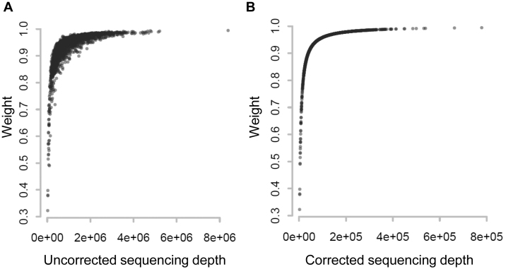
Based on our two-step weighting scheme, the weight for each cell is an increasing function of the corrected sequencing depth (), but not proportional to . In step (1), we set to obtain gene-specific and . In step (2), the final weight is updated as . The scatterplots in Figure 1 illustrate the relationship between the final weights and the sequencing depths. Specifically, we used 3005 scRNA-seq datasets from mouse cortex and hippocampus cells (20). The median weight across all genes within a cell is plotted against the uncorrected sequencing depth (i.e. the total number of mapped reads, Figure 1A) or the corrected sequencing depth (i.e. , Figure 1B). The weight usually increases as the raw sequencing depth increases, and it approached saturation when the raw sequencing depth is around two million (Figure 1A). Therefore, the contribution from cells saturates at high sequencing depths. This coincides with the observations that scRNA-seq libraries are close to saturation when raw sequencing depth is around 1∼2 million (24,25). As expected, the weight increases monotonically when the corrected sequencing depth increases (Figure 1B).

Figure 1.

Relationship between cell weight and sequencing depth. For each of the 3005 scRNA-seq, the median weight across all genes was calculated and plotted against (A) uncorrected sequencing depth (i.e. total number of mapped reads) or (B) corrected sequencing depth (i.e. ).

Accurate quantification and quality score assignment for gene expression measures of scRNA-seq

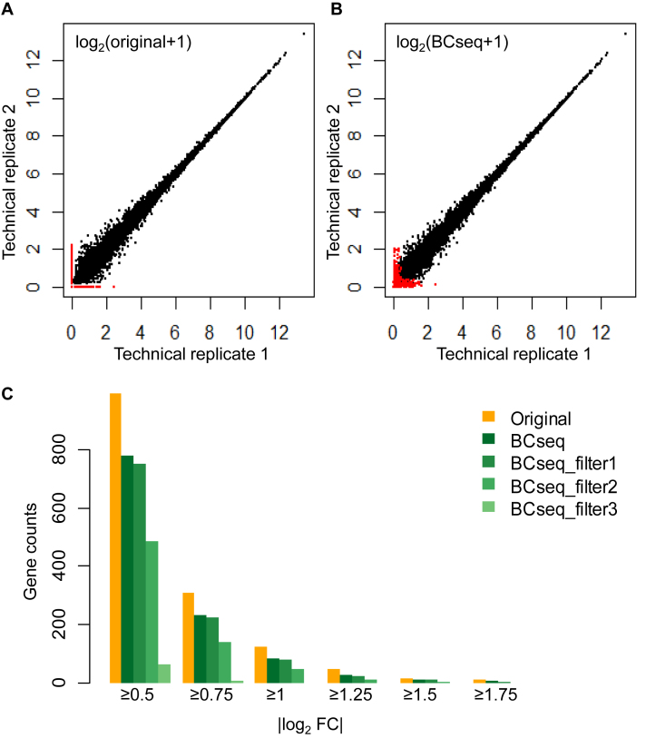
The lack of gold standard for single cell expression quantification makes it difficult to evaluate the performance of any analysis tool. Perhaps the best strategy to date was from Li et al. who carefully divided the transcriptome of a single neuron into two parts, as technical replicates, for separate scRNA-seq profiling (18). Ideally, expression measures of each gene from two technical replicates should be the same, since the RNA-seq libraries are sampled from the same cell. However, traditional TPM measures without bias correction led to many dropouts (red dots in Figure 2A, i.e. genes exhibiting non-negligible expression in one library and zero expression in the other library). The zero expression of a dropout is most likely due to sample loss during library preparation. These dropouts confound identification of truly differentially expressed genes, so require special attention.

Figure 2.

BCseq improves the consistency between two scRNA-seq technical replicates from the same cell. Comparison of the two technical replicates by (A) original STAR-derived TPM measures and (B) BCseq measures. Red dots represent dropouts that show high expression in one sample but zero expression in the other according to TPM measures. (C) Counts of genes with specified fold change (FC). The fold change is the TMP+1 or BCseq+1 ratio between two replicates. Different filters based on the BCseq quality measures were applied. The three filters are assigned according to the first quartile, the median, and the third quartile of all quality scores. Filter 1: consider genes with quality scores larger than −33.2 (i.e. first quartile of the quality scores) in both samples. Filter 2: consider genes with quality scores larger than −0.2 (i.e. median of the quality scores) in both samples. Filter 3: consider genes with quality scores larger than 1.5 (i.e. third quartile of the quality scores) in both samples.

Our BCseq model effectively handles these dropouts and decreases overall noises. BCseq utilizes information shared by the profiled cells (∼200 neurons in (18)) to derive a baseline expression level, which compensates for the effect of dropouts. The adjusted expression values from BCseq were more consistent between the two technical replicates, particularly for genes of lower expression (Figure 2B). As a result, less differentially expressed genes were identified between the two technical replicates. A total of 126 gene showed expression fold change ≥2 based on TPM measures following the STAR alignment, whereas only 85 genes met the same criterion based on BCseq measures (Figure 2C). The superior performance of BCseq between technical replicates was ubiquitous across a wide range of thresholds in determining differential expression (Figure 2C). Other normalization methods such as the trimmed mean of M values (TMM) (26) was applied for the fold change calculation. BCseq still identified the least number of DE genes (Supplementary Table S1). The advantage of BCseq measures was also independent of aligners, as BCseq outperformed TPM measures from the Kallisto alignment (Supplementary Figure S2).

BCseq assigns a quality measure to each expression estimation as an objective quality control parameter for downstream analysis. The quality measure is based on information entropy, which reflects the dispersion of the posterior distribution for gene expression in our modeling. By filtering out genes of low quality scores, we obtained more consistent expression values between the two technical replicates, and fewer genes exhibited expression fold changes (Figure 2C). Increasing the threshold for the quality measure (from filter 1 to filter 3) progressively improved the consistency between two replicates. Thus, the quality measure provides valuable information to guide selection of genes for downstream analysis.

Robust and powerful DE gene analysis of scRNA-seq

We compared BCseq to existing scRNA-seq analysis methods regarding identification of DE genes. Specifically, ROTS and BPSC were selected because they had been reported to be the best available tools for DE gene identification from scRNA-seq data (7,8). The current practice in the field utilizes scRNA-seq data mainly for comparison of cell type (or subtype) groups, where each cell group consists of a population of similar cells. In other words, the goal of DE gene analysis is to discern the difference between cell groups using their ‘averages’. Therefore, ‘bulk’ RNA-seq of a homogeneous cell group is a valid benchmark and probably the best standard. The comparison of two ‘single’ cells is less meaningful, because the derived information may not be generalized to other individual cells. Furthermore, comparison of two ‘single’ cells hardly has technical replicates for validation, because the cells would have been consumed by the scRNA-seq experiment.

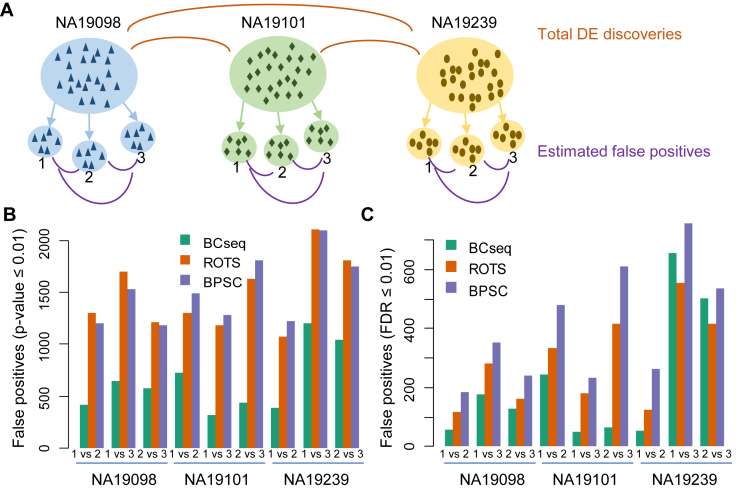
We chose the RNA-seq data set from Tung et al.'s study of three iPSC lines derived from three YRI individuals (NA19098, NA19101, and NA19239), which was specifically designed to study batch effect and scRNA-seq variance (19). In this well-designed data set, each cell line has 288 homogenous single-cell biological replicates experimented in the same condition but collected from three different 96-well plates (herein referred to groups 1, 2 and 3, Figure 3A). Thus, each cell line has three plate groups and each group has 96 replicates of scRNA-Seq. Three additional bulk RNA-seq replicates were also produced from a homogenous population of each cell line.

Figure 3.

False positive analysis within each cell line. (A) schematic for the experiment. Three different iPS cell lines were separately examined: NA19098, NA19101, and NA 19239. Each cell line contains three plate groups. Each group contains 96 scRNA-seq data. DE genes were identified by comparing groups within each cell line and were considered false positives. (B) P-value cut-off of 0.01 to declare DE genes. (C) FDR cut-off of 0.01 to declare DE genes.

False positives could be one of the biggest concerns in scRNA-seq analysis. We studied the false positive issue by comparing homogenous cell groups of the same cell line. We conducted three pair-wise group comparisons (‘1 versus 2’, ‘1 versus 3’ and ‘2 versus 3’) for each cell line (Figure 3A). Given this is a group comparison of the same cell line, a small number of differentially expressed genes (i.e. false positives) is expected. Surprisingly, ROTS and BPSC identified as large as a thousand of differentially expressed genes with P-value ≤ 0.01 (Figure 3B), many of which were presumably false positives. In contrast, BCseq identified drastically less false positives (Figure 3B). Application of a different statistical cutoff (FDR ≤ 0.01) obtained the same conclusion (Figure 3C), suggesting the superior performance of BCseq was independent of statistical cutoffs. When a fold change of >2.0 is further applied, the conclusion remains the same (Supplementary Figure S3).

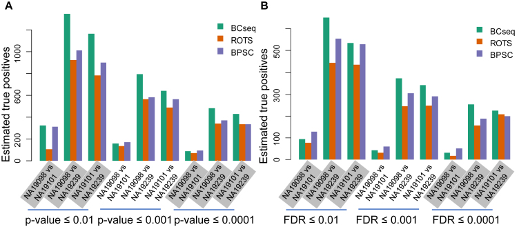
To assess the statistical power, we examined DE genes between different cell lines. First, we estimated the number of false positives by comparing plate groups of the same cell lines (‘1 versus 2’, ‘1 versus 3’ and ‘2 versus 3’). We then estimated the number of true positives as the total number of declared DE discoveries minus the number of estimated false positives (Figure 3A). As shown in Figure 4, BCseq always identified more true positives showing larger statistical power than other methods.

Figure 4.

Estimated statistical power for the DE analysis between different cell lines. For the comparison of different cell lines, the number of true positives was estimated as the total number of declared DE discoveries minus the estimated number of false positives. The number of false positives was estimated as the average number of false positives for the within-cell line comparison. (A) Different P-value cut-offs for the DE analysis. (B) Different FDR cut-offs for the DE analysis.

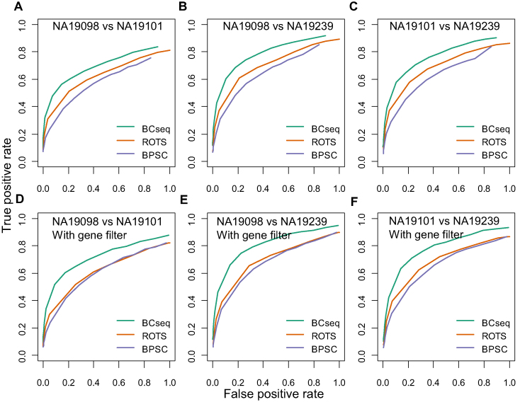
Because the bulk-cell RNA-seq had larger sequencing depths to compare cell lines, the identified DE genes could be more accurate and serve as a benchmark. Note that the ‘bulk’ RNA-seq used in our analysis profiled a homogenous cell population derived from a single cell clone instead of a heterogeneous population. Pair-wise comparison of NA19098, NA19101, and NA19239 using bulk-cell RNA-seq generated three lists of high-confident DE (true positive) and non-DE (true negative) genes between each pair. Subsequently, DE genes based on 288 (3 × 96) scRNA-seq of each cell line were identified by BCseq, ROTS and BPSC, separately. A more robust scRNA-seq analysis method should recover more true positives, given a specific false positive rate. As shown by the ROC curves in Figure 5, we observed widespread better performance from BCseq than ROTS and BPSC. When we considered genes with mean TPM ≥ 1 in the bulk RNA-seq for each cell line pairs, the superiority of BCseq was even more obvious (Figure 5D–F). Thus, BCseq exhibits clear advantages over other methods in identifying DE.

Figure 5.

Comparison of BCseq, ROTS and BPSC in DE analysis between different cell lines. ROC curves were based on ‘gold standards’ identified from bulk RNA-seq data. Each cell line (NA19098, NA19101, and NA19239) contains three bulk RNA-seq replicates with large sequencing depth. T-tests of DE genes were performed for each cell line pair. Genes with a P-value ≤ 0.01 are treated as true positives and genes with a P-value > 0.1 are treated as true negatives. DE analysis of scRNA-seq was performed by BCseq, ROTS, and BPSC, respectively. Each cell line contains 288 scRNA-seq. (A–C) all genes were considered. (D–F) only genes with average TPM measures across the three bulk RNA-seq replicates ≥1 for both cell lines were considered.

Cell clustering

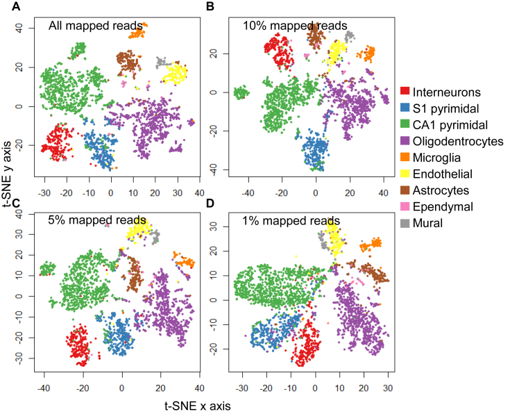
To test whether gene expression quantification from BCseq is sufficient for accurate cell type clustering, we chose the scRNA-seq dataset from mouse cortex and hippocampus because their cell type information was available (20). In Zeisel et al. (20), 3005 cells have been carefully separated into nine major classes or 47 subclasses based on known molecular markers and transcriptome profiling. In Figure 6A, we performed the t-SNE (23) dimension reduction and visualization with the BCseq expression values. BCseq clearly preserves the information necessary for accurate cell clustering. To test BCseq's robustness, we stressed the clustering by reducing sequencing depth. Strikingly, cell type separation based on BCseq was not affected by reducing input reads to only 10%, 5% or 1% total mapped reads (e.g. Figure 6B–D).

Figure 6.

T-SNE clustering and visualization of brain cells based on BCseq measures. (A) 100% mapped reads, (B) 10% of mapped reads, (C) 5% of mapped reads and (D) 1% of mapped reads were tested separately. BCseq accurately clusters cell subtypes in each scenario.

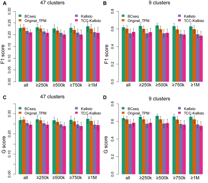
To further study the capability of BCseq to detect cell subtypes, we performed the spectral clustering (22) and calculated F1 and G scores to evaluate clustering strengths based on BCseq, STAR-derived TPM, Kallisto (gene-level expression), and TCC-Kallisto (normalized transcript-compatibility counts from Kallisto). F1 and G scores are harmonic and geometric means, respectively, of recall and precision, which are commonly used to evaluate classification accuracy. To increase the robustness of the comparison, we tested multiple scenarios altering the number of centers to be 9 or 47 as the original study classified these cells into nine major groups or 47 subclasses. Additionally, we varied the read number threshold of including cells into the F1 and G score calculation (i.e., all selected cells, or only cells with ≥250k, ≥500k, ≥750k or ≥1M mapped reads). We randomly selected one third of cells for spectral clustering and F1/G score calculation. The analysis was repeated 50 times to derive the means and standard deviations of F1 and G scores. As shown in Figure 7, the clustering performance based on BCseq is the best among the four measurements.

Figure 7.

Evaluation of clustering performance. One third of cells were randomly selected each time and the spectral clustering was repeated 50 times. Spectral clustering was performed on the sampled cells with (A, C) 47 centers or (B, D) nine centers. F1 score (A and B) and G score (C and D) were calculated based on the precision and recall values. We counted each cell pair as true positive (tp) or false positive (fp) based on whether they were correctly clustered together. We also counted true negatives (tn) and false negatives (fn) based on whether a cell pair was correctly assigned to different clusters. Precision is calculated as . Recall is calculated as . Then and . Five scenarios of cell inclusion for F1 and G score calculation are presented: all selected cell pairs (‘all’), cell pairs with more than 250k, 500k, 750k and 1M mapped reads per cell. The mean and standard deviation of F1 and G scores are shown.

DISCUSSION

ScRNA-seq analysis is hurdled by non-uniform read distribution, limited sequencing depth, and transcript loss during library preparation. BCseq tackled these challenges from multiple aspects. BCseq corrects inherent biases of RNA-seq via generalized Poisson modeling. BCseq takes advantage of large sample size in a typical scRNA-seq design to improve signal-to-noise ratio by allowing cells to borrow information from others. The two-step weighting scheme effectively assigns larger weights to cells of higher sequencing depth, which results in minimum variance for the estimator (i.e. bias-corrected TPM measure). Note that BCseq does not over-use ‘saturated’ cells containing more than 2 million reads. The posterior distribution of gene expression () incorporates baseline expression across multiple cells into individual cell-specific expression. These procedures benefit rescuing genes that are lost during library preparation.

In our bias correction, the generalized Poisson (GP) distribution assumes an underlying Poisson process with rate and a departure from the Poissonicity represented by the parameter . To understand the application of GP distribution in RNA-seq data analysis, we can treat an RNA-seq experiment as a branching process in which (i) the total number of RNA molecules in a sample is large, (ii) the probability of being selected to be amplified and sequenced is small for each molecule, (iii) each selected molecule becomes a spreader (biased to be more or less sequenced), (iv) the number of members in the group where each spreader is likely to spread is large. Then the total number of sequenced molecules in each group follows a GP distribution (27).

Although alternative splicing could result in uneven read distribution, but its contribution is significantly smaller than the RNA-seq experimental bias. We applied real data to test the impact of alternative splicing (more details in Supplementary Text). We found that the correlation between the read distribution heterogeneity and the expression was as high as 0.76. However, the correlation between the heterogeneity and the number of annotated alternative transcript isoforms was only 0.06. Therefore, the major contributor to the read count heterogeneity is experimental bias. Additionally, our studies of false positives based on scRNA-seq replicates show that BCseq outperforms other methods for both single-isoform genes and multi-isoform genes (Supplementary Figures S4 and S5). Therefore, our handling of the bias is still valid without consideration of alternative splicing. If a large number of alternative splicing events are suspected for a certain experiment, users could simply use constitutive exons and exclude alternative exons for the analysis.

The comparisons of BCseq to existing methods demonstrate the robustness of BCseq. Due to high noises and non-uniform read distribution of scRNA-seq, high false positives in DE analysis remain a significant challenge, as highlighted by the analysis of homogenous cells from the same iPS cell clone (Figure 3). With the best reported methods (ROTS and BPSC), falsely declared differentially expressed genes were in thousands (P-value < 0.01) or hundreds (FDR < 0.01). BCseq significantly reduced the number of false positives (Figure 3). The true positive (Figure 4) and ROC analysis further (Figure 5) demonstrated the robustness of BCseq on both false positive control and statistical power.

The more accurate single-cell transcriptome comparison is essential for the detection of cell-to-cell variation. Indeed, BCseq is the best among all considered measurements to produce robust cell clustering, as assayed by F1 and G scores (Figure 7). We note that current cell clustering approaches are still imperfect to detect subtle subtypes from similar cells. For example, the F1 score for the cluster analysis of 47 centers is much smaller than for the cluster analysis of nine centers (0.2 versus 0.6 in Figure 7), indicating a need for more powerful clustering methods.

In addition to improving expression quantification, we included a quality measure based on information entropy. The information entropy reflects the dispersion of the posterior distribution for gene expression , which provides useful information for prioritizing gene candidates and downstream analysis. For example, in addition to P-values and fold changes, users can include the information-entropy-based quality measures to prioritize DE genes (e.g. genes with high quality measures).

In summary, we propose BCseq for accurate gene expression quantification of scRNA-seq. BCseq is a powerful tool that significantly improves DE analysis and cell clustering of scRNA-seq experiments.

DATA AVAILABILITY

The public scRNA-seq data used in this study are from the NCBI GEO database (https://www.ncbi.nlm.nih.gov/geo/) including GSE63576 (Li et al., 2016), GSE77288 (Tung et al., 2017), and GSE60361 (Zeisel et al., 2015). Our software tool BCseq is available at http://www-rcf.usc.edu/∼liangche/software.html.

SUPPLEMENTARY DATA

Supplementary Data are available at NAR Online.

FUNDING

National Institutes of Health [R01GM097230 and R01MH116220 to L.C. and R00MH096807 and R01NS104041 to S.Z.]. Funding for open access charge: National Institutes of Health.

Conflict of interest statement. None declared.

REFERENCES

- 1. Yang J., Tanaka Y., Seay M., Li Z., Jin J., Garmire L.X., Zhu X., Taylor A., Li W., Euskirchen G. et al. . Single cell transcriptomics reveals unanticipated features of early hematopoietic precursors. Nucleic Acids Res. 2017; 45:1281–1296. [DOI] [PMC free article] [PubMed] [Google Scholar]
- 2. Song Y., Botvinnik O.B., Lovci M.T., Kakaradov B., Liu P., Xu J.L., Yeo G.W.. Single-Cell alternative splicing analysis with expedition reveals splicing dynamics during neuron differentiation. Mol. Cell. 2017; 67:148–161. [DOI] [PMC free article] [PubMed] [Google Scholar]
- 3. Stegle O., Teichmann S.A., Marioni J.C.. Computational and analytical challenges in single-cell transcriptomics. Nat. Rev. Genet. 2015; 16:133–145. [DOI] [PubMed] [Google Scholar]
- 4. Srivastava S., Chen L.. A two-parameter generalized Poisson model to improve the analysis of RNA-seq data. Nucleic Acids Res. 2010; 38:e170. [DOI] [PMC free article] [PubMed] [Google Scholar]
- 5. Zhang J., Kuo C.C., Chen L.. WemIQ: an accurate and robust isoform quantification method for RNA-seq data. Bioinformatics. 2015; 31:878–885. [DOI] [PMC free article] [PubMed] [Google Scholar]
- 6. Bacher R., Kendziorski C.. Design and computational analysis of single-cell RNA-sequencing experiments. Genome Biol. 2016; 17:63. [DOI] [PMC free article] [PubMed] [Google Scholar]
- 7. Jaakkola M.K., Seyednasrollah F., Mehmood A., Elo L.L.. Comparison of methods to detect differentially expressed genes between single-cell populations. Brief. Bioinformatics. 2017; 18:735–743. [DOI] [PMC free article] [PubMed] [Google Scholar]
- 8. Vu T.N., Wills Q.F., Kalari K.R., Niu N., Wang L., Rantalainen M., Pawitan Y.. Beta-Poisson model for single-cell RNA-seq data analyses. Bioinformatics. 2016; 32:2128–2135. [DOI] [PubMed] [Google Scholar]
- 9. Seyednasrollah F., Rantanen K., Jaakkola P., Elo L.L.. ROTS: reproducible RNA-seq biomarker detector-prognostic markers for clear cell renal cell cancer. Nucleic Acids Res. 2016; 44:e1. [DOI] [PMC free article] [PubMed] [Google Scholar]
- 10. Finak G., McDavid A., Yajima M., Deng J., Gersuk V., Shalek A.K., Slichter C.K., Miller H.W., McElrath M.J., Prlic M. et al. . MAST: a flexible statistical framework for assessing transcriptional changes and characterizing heterogeneity in single-cell RNA sequencing data. Genome Biol. 2015; 16:278. [DOI] [PMC free article] [PubMed] [Google Scholar]
- 11. Kharchenko P.V., Silberstein L., Scadden D.T.. Bayesian approach to single-cell differential expression analysis. Nat. Methods. 2014; 11:740–742. [DOI] [PMC free article] [PubMed] [Google Scholar]
- 12. Anders S., Huber W.. Differential expression analysis for sequence count data. Genome Biol. 2010; 11:R106. [DOI] [PMC free article] [PubMed] [Google Scholar]
- 13. Smyth G.K. Linear models and empirical bayes methods for assessing differential expression in microarray experiments. Stat. Applic. Genet. Mol. Biol. 2004; 3:Article3. [DOI] [PubMed] [Google Scholar]
- 14. Robinson M.D., McCarthy D.J., Smyth G.K.. edgeR: a Bioconductor package for differential expression analysis of digital gene expression data. Bioinformatics. 2010; 26:139–140. [DOI] [PMC free article] [PubMed] [Google Scholar]
- 15. Dobin A., Davis C.A., Schlesinger F., Drenkow J., Zaleski C., Jha S., Batut P., Chaisson M., Gingeras T.R.. STAR: ultrafast universal RNA-seq aligner. Bioinformatics. 2013; 29:15–21. [DOI] [PMC free article] [PubMed] [Google Scholar]
- 16. Bray N.L., Pimentel H., Melsted P., Pachter L.. Near-optimal probabilistic RNA-seq quantification. Nat. Biotechnol. 2016; 34:525–527. [DOI] [PubMed] [Google Scholar]
- 17. Ntranos V., Kamath G.M., Zhang J.M., Pachter L., Tse D.N.. Fast and accurate single-cell RNA-seq analysis by clustering of transcript-compatibility counts. Genome Biol. 2016; 17:112. [DOI] [PMC free article] [PubMed] [Google Scholar]
- 18. Li C.L., Li K.C., Wu D., Chen Y., Luo H., Zhao J.R., Wang S.S., Sun M.M., Lu Y.J., Zhong Y.Q. et al. . Somatosensory neuron types identified by high-coverage single-cell RNA-sequencing and functional heterogeneity. Cell Res. 2016; 26:83–102. [DOI] [PMC free article] [PubMed] [Google Scholar]
- 19. Tung P.Y., Blischak J.D., Hsiao C.J., Knowles D.A., Burnett J.E., Pritchard J.K., Gilad Y.. Batch effects and the effective design of single-cell gene expression studies. Scientific Rep. 2017; 7:39921. [DOI] [PMC free article] [PubMed] [Google Scholar]
- 20. Zeisel A., Munoz-Manchado A.B., Codeluppi S., Lonnerberg P., La Manno G., Jureus A., Marques S., Munguba H., He L., Betsholtz C. et al. . Brain structure. Cell types in the mouse cortex and hippocampus revealed by single-cell RNA-seq. Science. 2015; 347:1138–1142. [DOI] [PubMed] [Google Scholar]
- 21. Liao Y., Smyth G.K., Shi W.. featureCounts: an efficient general purpose program for assigning sequence reads to genomic features. Bioinformatics. 2014; 30:923–930. [DOI] [PubMed] [Google Scholar]
- 22. Karatzoglou A., Smola A., Hornik K., Zeileis A.. kernlab - An S4 package for kernel methods in R. J. Stat. Softw. 2004; 11:1–20. [Google Scholar]
- 23. van der Maaten L. Accelerating t-SNE using Tree-Based algorithms. J. Mach. Learn. Res. 2014; 15:3221–3245. [Google Scholar]
- 24. Ziegenhain C., Vieth B., Parekh S., Reinius B., Guillaumet-Adkins A., Smets M., Leonhardt H., Heyn H., Hellmann I., Enard W.. Comparative analysis of Single-Cell RNA sequencing methods. Mol. Cell. 2017; 65:631–643. [DOI] [PubMed] [Google Scholar]
- 25. Wu A.R., Neff N.F., Kalisky T., Dalerba P., Treutlein B., Rothenberg M.E., Mburu F.M., Mantalas G.L., Sim S., Clarke M.F. et al. . Quantitative assessment of single-cell RNA-sequencing methods. Nat. Methods. 2014; 11:41–46. [DOI] [PMC free article] [PubMed] [Google Scholar]
- 26. Robinson M.D., Oshlack A.. A scaling normalization method for differential expression analysis of RNA-seq data. Genome Biol. 2010; 11:R25. [DOI] [PMC free article] [PubMed] [Google Scholar]
- 27. Consul P.C., Famoye F.. Lagrangian Probability Distribution. 2006; Basel: Birkhäuser. [Google Scholar]
Associated Data
This section collects any data citations, data availability statements, or supplementary materials included in this article.
Supplementary Materials
Data Availability Statement