Deep Neural Networks for Ultrasound Beamforming

Abstract

We investigate the use of deep neural networks (DNNs) for suppressing off-axis scattering in ultrasound channel data. Our implementation operates in the frequency domain via the short-time Fourier transform. The inputs to the DNN consisted of the separated real and imaginary components (i.e. in-phase and quadrature components) observed across the aperture of the array, at a single frequency and for a single depth. Different networks were trained for different frequencies. The output had the same structure as the input and the real and imaginary components were combined as complex data before an inverse short-time Fourier transform was used to reconstruct channel data. Using simulation, physical phantom experiment, and in vivo scans from a human liver, we compared this DNN approach to standard delay-and-sum (DAS) beamforming and an adaptive imaging technique that uses the coherence factor (CF).

For a simulated point target, the side lobes when using the DNN approach were about 60 dB below those of standard DAS. For a simulated anechoic cyst, the DNN approach improved contrast ratio (CR) and contrast-to-noise (CNR) ratio by 8.8 dB and 0.3 dB, respectively, compared to DAS. For an anechoic cyst in a physical phantom, the DNN approach improved CR and CNR by 17.1 dB and 0.7 dB, respectively. For two in vivo scans, the DNN approach improved CR and CNR by 13.8 dB and 9.7 dB, respectively. We also explored methods for examining how the networks in this work function.

I. INTRODUCTION

The delay-and-sum (DAS) beamformer is the standard method for combining ultrasound array channel signals into the ultrasound radio-frequency (RF) signals used to create a B-mode image. The algorithm consists of applying phase delays and weights to each channel before channel signal summation. The phase delays are used to focus the beam on receive and the channel weights are used to control the beam characteristics, including main lobe width and side lobe levels.

Sources of ultrasound image degradation such as off-axis scattering, multi-path reverberation, and phase aberration limit the clinical use of ultrasound imaging. For this reason, numerous techniques have been proposed to improve ultrasound image quality [1], [2], [3], [4]. Few of these techniques have transferred to the clinic. One notable exception is harmonic imaging, which discards all of the useful information at the fundamental frequency and forms images using the second harmonic waveform generated from non-linear propagation.

Byram et al. developed a model based beamforming method called aperture domain model image reconstruction (ADMIRE) [4], [5]. They tuned ADMIRE to improve ultrasound image quality by suppressing sources of image degradation. In addition, the development of ADMIRE demonstrated that beamforming could be posed as a nonlinear regression problem, which suggests that a deep neural network (DNN) might be used to accomplish the same task. This is important because ADMIRE is relatively inefficient. In contrast, DNNs take a long time to train but once trained can be implemented efficiently.

Recently, DNNs have been used to improve the state of the art in applications such as image classification [6], speech recognition [7], natural language processing [8], object detection [9], and others. DNNs consist of cascaded layers of artificial neurons. Although individual artificial neurons are simplistic processing units, when combined in a single layer network, they can be used to approximate any continuous function [10]. The potential contributions of DNNs to medical image classification have been and continue to be investigated [11]. In contrast, the impact of DNNs on medical image reconstruction are just starting to be examined [12], [13]. The goal of this paper was to significantly expand and report on our previous work to integrate DNNs into an ultrasound beamformer and to train them to improve the quality of the resulting ultrasound images [14].

II. METHODS

A Frequency domain sub-band processing

Several methods have relied on processing ultrasound channel data in the frequency domain to offer improvements to ultrasound image quality. For example, Holfort et al. applied the minimum variance (MV) beamforming technique in the frequency domain to improve ultrasound image resolution [15]. Shin et al. applied frequency space prediction filtering in the frequency domain to suppress acoustic clutter and noise [16]. ADMIRE also operates in the frequency domain to suppress off axis scattering and reverberation [4], [5].

A flow chart for the proposed DNN approach is in Fig. 1. Frequency domain minimum variance beamforming, frequency space prediction filtering, and ADMIRE have similar flow charts, except that the middle step is unique to each method. In each method, a short-time Fourier transform (STFT) is used to produce sub-band data in the frequency domain, which is processed in some way to suppress acoustic clutter and improve ultrasound image quality. Next, an inverse short-time Fourier transform (ISTFT) is used to convert back to the time-domain. In this work, DNNs ere trained to suppress off-axis scattering.

Fig. 1.

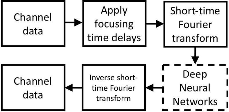
Flow chart for the proposed DNN approach.

We used an STFT window length of one pulse length, the STFT window overlap was 90%, the window was rectangular, and no padding was used. The least squares ISTFT described by Yang was used to transform back to the time domain [17]. A diagram showing the frequency domain processing for a single depth of channel data (i.e., axially gated channel data from one depth) is in Fig. 2.

Fig. 2.

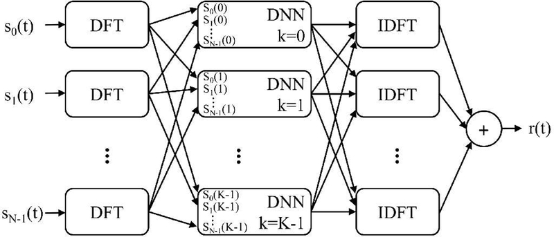
Frequency domain processing, where the inputs were a single axially gated section of channel data. Each channel was transformed into the frequency domain using the discrete Fourier transform (DFT). DNNs specific to each DFT frequency and trained to suppress off-axis scattering removed clutter. The data was transformed back into the time domain using an inverse discrete Fourier transform (IDFT). Note that the IDFT and summation operations could be interchanged.

B. Neural Networks

We trained a different network for each frequency and the real and imaginary components of the signals were treated as separate inputs to the network as in Fig. 3 (a). Therefore, if the array had N elements, the number of network inputs was 2N The configuration of the network output was the same as that of the network input, i.e., separated real and imaginary data.

Fig. 3.

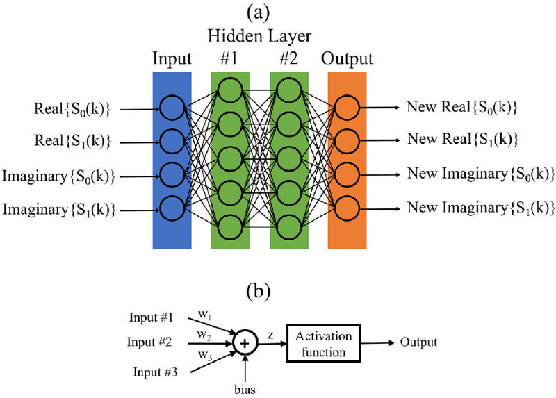
(a) Example feed-forward multi-layer fully connected network setup for a two element array. The inputs to the network were separated into real and imaginary components. Information only moves from left to right. (b) Diagram for a single neuron.

We used feed-forward multi-layer fully connected networks in this work. In this type of network topology, each neuron in one layer has directed connections to the neurons in the next layer as shown in Fig. 3 (a). Depending on the number of hidden layers and the width of each hidden layer, a network may have hundreds or even thousands of neurons. A single neuron is simplistic processing unit that consists of a summation operation over the inputs followed by an activation function that nonlinearly maps to the output as shown in Fig. 3 (b).

We performed a hyperparameter search with parameters in the ranges indicated in Table I. A variant of stochastic gradient descent (SGD), called Adam, was used to train the neural networks in this work with mean-squared error (MSE) as the loss function [18]. An early stopping criterion was employed, where training was terminated if network performance did not improve based on the validation loss after 20 epochs. For each training epoch, the network was saved only if the validation loss was the best obtained up to that point in the training. In this way, the network with the best validation loss was produced at the end of training.

Table I.

HYPERPARAMETER SEARCH SPACE

Parameter	Search Values
Hidden Layers	1–5
Layer Widths	65–260 (multiples of 5)
Learning Rate	10−5 − 10−2
Learning Rate Decay	10−8 − 10−5
Dropout Probability	0–0.5
Weight Initializations	Normal, Uniform  He Normal, He Uniform

To create and train the networks in this work, we used Keras, a high-level neural network API written in Python [19], with TensorFlow as the backend [20]. Training was performed on a GPU computing cluster maintained by the Advanced Computing Center for Research and Education at Vanderbilt University.

Selection of the network activation function is an important design choice and neural network activation functions are still an active area of research [21], [22]. An activation function determines whether a neuron activates or not based on the value of the weighted sum of inputs. We used the rectified linear unit (ReLU) as the activation function for the networks in this work, given as

$$g\left(z\right)=\max \left\{0,z\right\}$$ (1)

where z is the summation output. The rectified linear unit is a nonlinear function; however, it is composed of two linear parts and is easier to optimize with gradient-based optimization methods compared to other activation functions such as the hyperbolic tangent [23]. The shape of the rectified linear unit is in Fig. 4. A linear activation function was used for the neurons in the output layer.

Fig. 4.

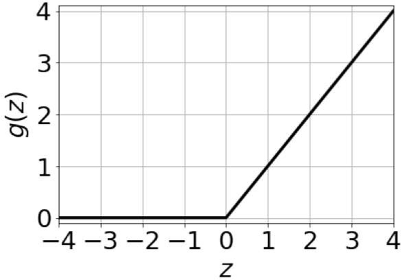
Rectified linear unit.

Dropout is an effective technique for preventing a neural network, which may have a large number of adjustable weights, from overfitting and memorizing the training data [24]. When using dropout, neurons and their connections are randomly removed from the network according to a given dropout probability during the training phase (dropout is not used during the testing phase, i.e., when evaluating the networks on the validation and test data sets, and once the networks are deployed). Reports in the literature on the effectiveness of dropout for regression problems are sparse or nonexistent¹. We varied the dropout probability to study if dropout was useful for the application in this work.

Before training a neural network, the parameter weights of the network need to be initialized to a starting value. One option is to randomly initialize the weights using a Normal distribution or Uniform distribution. There exist other initialization methods that take into account the activation function of choice. He et al. developed a weight initialization methods for activation functions in the rectified linear unit family [21]. We examined using weights initialized using a Gaussian distribution, a Uniform distribution and the initialization methods developed by He et al. for rectified linear units.

C. Training Data

Training was conducted in a supervised manner, where a network was shown paired input and output examples. The training process for deep neural networks requires a large data set. Such data sets do not exist for the problem studied in this work and obtaining an experimental training data set for this application would be very time consuming or even impossible. Therefore, we used simulation to generate training, validation, and test data sets. FIELD II was used to simulate the responses from point targets placed in the field of a linear array transducer having the parameters given in Table II [26]. The point targets were randomly positioned along the annular sector in Fig. 5. The center radius of the annular sector was set to be equal to the transmit focal depth. The goal was to train a network for the STFT depth that was centered at the transmit focal depth. For point targets positioned as described and for the central elements of the array, the received signal will be centered in the depth at the transmit focus. To expand the depth of field of the network and to take into account some of the offset effects from using a STFT window, the width of the annular sector was two pulse lengths.

Table II.

LINEAR ARRAY PARAMETER VALUES

Parameter	Value
Active Elements	65
Transmit Frequency	5.208 MHz
Pitch	298 µm
Kerf	48 µm
Simulation Sampling Frequency	520.8 MHz
Experimental Sampling Frequency	20.832 MHz
Speed of Sound	1540 m/s
Transmit Focus	70 mm

Fig. 5.

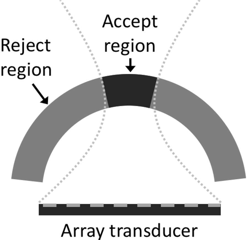
Scatterers were randomly placed along the annular sector as depicted. The acceptance region was taken as the region between the first nulls of a simulated beam.

Acceptance and rejection regions were defined based on the characteristics of the transducer as shown in Fig. 5. The acceptance region consisted of the main lobe width as measured by the first null of a simulated beam for the array at the transmit center frequency. The acceptance region and rejection were kept the same for all frequencies.

FIELD II was used to simulate the channel data for an individual point target. The channel data was gated using a window centered at the transmit focus and having a temporal length that was one pulse length long. A fast Fourier transform was used to convert the data into the frequency domain.

For point targets located in the acceptance region, the desired output was exactly same as the input. For point targets located in the rejection region, the desired output was equal to zero at all output nodes. In this way, the network was asked to return the input if the point target was in the acceptance region and to completely suppress the output if the point target was in the rejection region.

The training data set consisted of the simulated individual responses from 100,000 point targets randomly positioned in the annular sector in Fig. 5. This data set was only used during the network training phase, specifically to adjust the network weights. Half of the point targets were in the acceptance region and the other half in the rejection region. Although the rejection region had greater area compared to the acceptance region, dividing the data in this manner maintained balanced classes. Our experience indicates that it is more difficult to accurately reconstruct signals than to suppress signals, suggesting that it may be advantageous to have higher density training data in the acceptance region.

The validation data set consisted of the simulated individual responses from 25,000 different point targets randomly positioned along the annular sector in Fig. 5. Half of them were in the acceptance region and the other half in the reject region. This data set was only used during the training phase and for model selection. At the end of each training epoch, the validation data set loss was computed and used to determine when to stop training the network. If after 20 epochs, the validation loss did not improve, the training phase for the network was terminated. In addition, after each epoch, the current weights for the network were saved if validation loss decreased below that of the previous best epoch validation ultrasound channel data.

The test data set had the same setup as the validation data set, except that the responses from 25,000 point targets that had different positions compared to those in the validation data set were simulated. The test data was only used to report the performance of the final selected model.

White Gaussian noise was added to batches of training, validation, and test data with variable SNR in the range 0–60 dB. It should be noted that the training, validation, and test data sets used in this work consisted of the responses from individual point targets. Networks were never trained or evaluated using the response from multiple point targets as would be expected in a diffuse scattering scenario.

The training, validation, and test data sets were normalized in the following way. For each point target, the absolute value was taken of the separated real and imaginary components and the maximum value was found. The real and imaginary components were divided by this maximum value. During deployment, aperture domain signals were normalized using this same method and then rescaled using the normalizing constant after being processed by a network.

D. Transfer Learning

The first network that we trained was for the transmit center frequency using the process described in the previous sections. Instead of starting from scratch to train networks at other frequencies, we initialized a network for a new analysis frequency using the weights from a network trained for a different analysis frequency. The advantage of this approach is that it is quicker to adjust the weights of an already trained network than it is to start from scratch, all of the networks have the same architecture, and only the weights have been adjusted based on the frequency that the network was trained to process.

E. Coherence Factor

As an additional comparison besides standard DAS, we also include the coherence factor (CF), which is an adaptive imaging method that suppresses clutter by exploiting the fact that non-clutter signals exhibit longer spatial coherence across the aperture compared to clutter signals [1], [2]. The coherence factor is defined as

$$CF=\frac{{\left|{\displaystyle {\sum }_{i=0}^{N-1}S\left(i\right)}\right|}^2}{N{\displaystyle {\sum }_{i=0}^{N-1}{\left|S\left(i\right)\right|}^2}}$$ (2)

where N is the number of elements in the subaperture, S(i) is the received signal after receive delays have been delayed, and i is the index for the receive channel. Images were formed by multiplying the coherence factor in Eq. 2 by radio frequency data that was beamformed using DAS and then taking the envelope. Images created using the coherence factor were included in this paper to serve as a comparison between the DNN beamformer and other adaptive beamformers.

F. Image Quality Metrics

Image quality was quantified using contrast ratio (CR) as

$$CR=-20{\log }_{10}\left(\frac{{\mu }_{lesion}}{{\mu }_{background}}\right),$$ (3)

contrast-to-noise ratio (CNR) as

$$CNR=20{\log }_{10}\left(\frac{\left|{\mu }_{background}-{\mu }_{lesion}\right|}{\sqrt{{\sigma }^2{}_{background}+{\sigma }^2{}_{lesion}}}\right),$$ (4)

and speckle signal-to-noise ratio (SNRs) as

$$SNRs=\frac{{\mu }_{background}}{{\sigma }_{background}},$$ (5)

where µ is the mean of the envelope and σ is the standard deviation of the uncompressed envelope.

G. Simulations

The training, validation, and test data sets used for network training and evaluation purposes were generated using a simulated array transducer that was modeled after an ATL L7–4 38 mm linear array transducer and with properties in Table II. Field II was used to generate these data sets and to create channel data sets for point targets and diffuse scattering scenarios to show the capability of the trained neural networks.

For the point target simulation, a point target was placed at the transmit focus for the array. The point target was imaged using beams that were separated by one pitch length. White Gaussian noise was added to the simulated data so that the channel SNR was 50 dB.

For the cyst simulation, a 5 mm diameter spherical anechoic cyst was centered at a depth of 70 mm. The region around the cyst was filled with scatterers having density of 25 scatterers per resolution cell and zero scatterers were placed inside the cyst. The cyst was imaged using beams separated by one pitch length. A total of five anechoic cysts were scanned. White Gaussian noise was added to the simulated data so that the channel SNR was 20 dB.

H. Phantom Experiment

A linear array transducer (ATL L7-4 38 mm) was operated using a Verasonics Vantage 128 system (Verasonics, Kirkland, WA) to scan a 5 mm diameter cylindrical anechoic cyst at a depth of 70 mm in a physical phantom. The physical phantom was a multipurpose phantom (Model 040GSE, CIRS, Norfolk, VA) having 0.5 dB/cm of attenuation. The same scanning configuration was used for the phantom experiment as was used in the simulations. A total of 14 scans were made at different positions along the long axis of the cylindrical cyst.

I. In vivo Experiment

A linear array transducer (ATL L7-4 38 mm) was operated using a Verasonics Vantage 128 system (Verasonics, Kirkland, WA) to scan the liver of a 36 year old healthy male. The scans were conducted to look for vasculature in the liver. The same scanning configuration was used for the in vivo experiment as was used in the phantom experiment. The study was approved by the local Institutional Review Board.

III. RESULTS

A. Hyperparameter Search

Networks were trained using the transducer characteristics in Table II. A total of 100 neural networks were trained using the hyperparameter search in Table I. The parameters for the network with the lowest validation loss are in Table III and the MSE of the selected network for the training, validation, and test data sets were 1.8 × 10⁻⁴, 2.1 × 10⁻⁴, and 2.5 × 10⁻⁴, respectively. The training and validation loss functions for the network with the lowest validation loss are in Fig. 6, which provides strong evidence that the selected network did not suffer from overfitting.

Table III.

BEST NETWORK PARAMETER VALUES

Parameter	Value
Hidden Layers	5
Layer Width	170
Learning Rate	1.1 × 10−3
Learning Rate Decay	4.1 × 10−8
Dropout Probability	4.4 × 10−4
Weight Initialization	He Normal

Fig. 6.

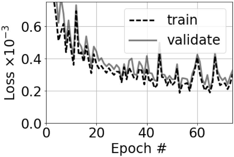
Training and validation loss functions for the network with the lowest validation loss.

Validation loss as a function of the hyperparameter search space is in Fig. 7. Fig. 7 (a) shows a positive correlation between dropout and validation loss, suggesting that dropout was not beneficial while training the networks in this work. Fig. 7 (c) suggests that the learning rate should be on the order of 10⁻³ or less.

Fig. 7.

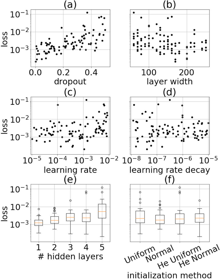
Validation loss as a function of hyperpameter search space.

Fig. 7 (b) shows a weak negative correlation between layer width and validation loss, suggesting that there was a benefit to increasing layer width. Fig. 7 (e) shows that on average the lowest validation loss resulted for single layer networks. However, it should be noted that out of the five best performing networks, four of them had three or more hidden layers. These findings suggest that the larger networks performed better than the smaller networks, which is consistent with previous work on the loss surfaces of neural networks. Choromanska et al. suggested that larger networks have loss surfaces with many local minima that are easy to find and have similar performance in terms of validation loss, while smaller networks have fewer minima that are harder to find and poor performance in terms of validation loss [27].

After selecting the best performing network, we used this network to train networks for the other analysis frequencies as described Section II-D. Typically, this took a single hyperparameter tuning step to modify the weights of the network such that it had similar performance for the new frequency. The STFT gate length was 16 samples, which was approximately one pulse length, for all of the examples in this work, including the training, validation, and testing data sets. A 16 point DFT was used. The first network that we trained was for the transmit center frequency. Because the input sequence was real, the DFT is conjugate symmetric. Therefore, we trained a total of nine networks and used the redundancy of the DFT to assign values for the remaining frequencies.

B. Simulated Point Target

Simulated point target images using DAS and the DNN approach are in Fig. 8. The tails that are characteristic for DAS point target images are clearly visible in Fig. 8 (a) and they have been suppressed in Fig. 8 (c) using DNNs. The axially integrated lateral profile is in Fig. 8 (d) and shows that side lobes were suppressed by approximately 60 dB when using the DNN approach compared to standard DAS and by approximately 40 dB compared to CF. The axial profile through the center of the point target is in Fig. 8 (e) shows that the axial response when using the DNN approach were about 15 dB higher than those observed when using DAS and CF.

Fig. 8.

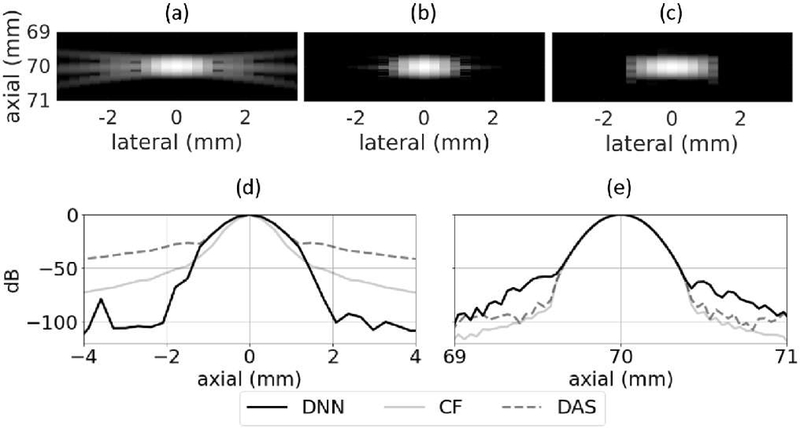
Point target using (a) DAS, (b) CF, and (c) DNNs. (d) Axially integrated lateral profile and (e) axial profile through the center of the point target. White Gaussian noise was added to the channel data so that the channel SNR was 50 dB. Images are shown with a 60 dB dynamic range.

In general, these results show the potential of the DNN approach for suppressing side lobes for individual point targets. The networks were trained using the responses from single point targets and the images in Fig. 8 show that the DNNs successfully accomplished the task they were trained to do.

C. Simulated Anechoic cyst

The set of networks that was trained using the responses from individual point targets was applied to simulated ane choic cysts. Example cyst images produced using DAS, CF, and the proposed DNN approach are in Fig. 9. In addition, contrast ratio, contrast-to-noise ratio, and speckle SNR values when using DAS, CF, and DNNs are in Table IV, which shows mean and standard deviation values for five simulated cysts.

Fig. 9.

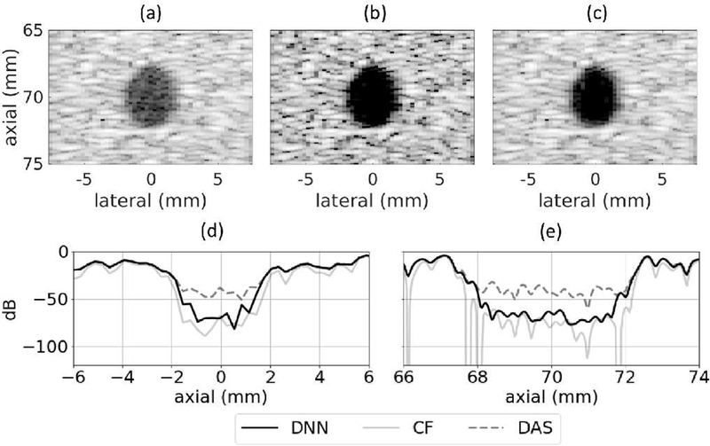
Simulated 5 mm diameter anechoic cyst at 70 mm depth using (a) DAS, (b) CF, and (c) DNNs. (d) Lateral and (e) axial profiles through the center of the cyst. White Gaussian noise was added such that the channel SNR was 20 dB. Images are shown with a 60 dB dynamic range.

Table IV.

SPECKLE STATISTICS FOR SIMULATED ANECHOIC CYSTS

Parameter	DAS	CF	DNN
CR (dB)	25.9 ± 0.6	42.6 ± 1.8	34.7 ± 1.3
CNR (dB)	5.2 ± 0.4	3.0 ± 0.3	5.5 ± 0.4
Speckle SNR	1.93 ± 0.08	1.43 ± 0.05	1.92 ± 0.08

Compared to standard DAS, the DNN approach improved contrast ratio by 8.8 dB and improved contrast-to-noise by 0.3 dB, while preserving speckle SNR. It should be noted that the best achievable CNR without altering background speckle is the theoretical value for the SNR of a Rayleigh distribution, approximately 5.6 dB. The DNN approach almost achieves this optimal value. There was a statistically significant difference as measured by a paired samples t-test between the DAS and DNN images for contrast ratio (df = 4, t = 19.1, p = 4 ×10⁻⁵) and for contrast-to-noise ratio (df = 4; t = 17.6, p = 6×10⁻⁵). There was also a statistically significant difference between the CF and DNN images for contrast ratio (df = 4, t = −22.9, p = 2 × 10⁻⁵) and for contrast-to-noise ratio (df = 4, t = 49.0, p = 1 × 10⁻⁶). The axial and lateral profiles in Fig. 9 (d) and (e) show that the DNN envelope was about 30 dB below that of standard DAS near the center of the cyst, indicating that the DNNs offered suppression of off-axis scattering relative to standard DAS. In addition, comparing the background speckle regions when using standard DAS and the proposed DNN approach, the DNN approach produced a speckle pattern that was very similar to that produced by standard DAS. The CF method produced a larger improvement in contrast ratio than did DNNs; however, it did so at the expense of CNR and speckle SNR, which were significantly lower compared to DAS. The tradeoff of CNR for contrast is a common trend with adaptive beamformers and can hinder visualization.

D. Phantom Anechoic Cyst

The set of networks that was trained using simulated training data was applied to an experimental scan from a physical phantom. The images produced using standard DAS, CF, and the proposed DNN approach are in Fig. 10. Contrast ratio, contrast-to-noise ratio, and speckle SNR are in Table V. When using the proposed DNN approach compared to standard DAS, contrast ratio improved by 17.1 dB, contrast-to-noise ratio increased by 0.7 dB, and speckle SNR decreased 0.06. There was a statistically significant difference as measured by a paired samples t-test between the DAS and DNN images for contrast ratio (df = 13, t = 18.7, p = 9 × 10⁻¹¹) and for contrast-to-noise ratio (df = 13, t = 24.5, p = 3 × 10⁻¹²). There was also a statistically significant difference between the CF nd DNN images for contrast ratio (df = 13, t = 7.0, p = 8 × 10⁻¹¹) and for contrast-to-noise ratio (df = 13, t = 73.3, p = 2 × 10⁻¹⁸).

Fig. 10.

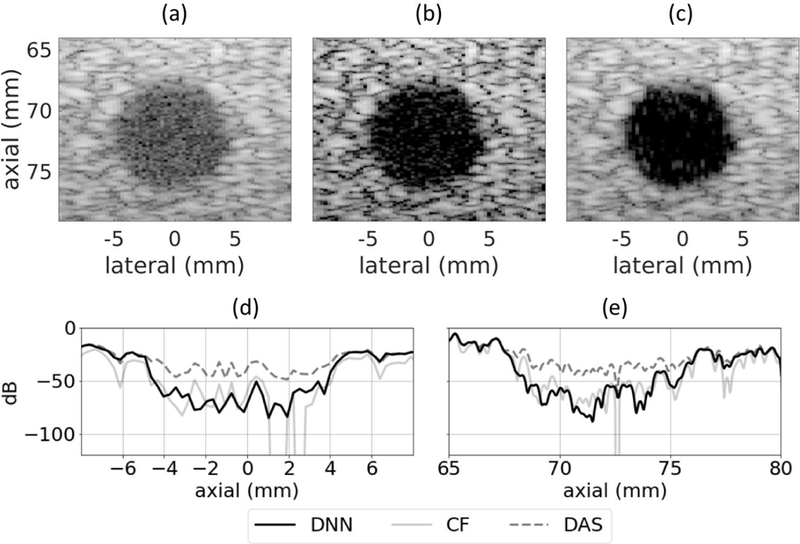
Phantom 5 mm diameter anechoic cyst at 70 mm depth using (a) DAS, (b) CF, and (c) DNNs. (d) Lateral and (e) axial profiles through the center of the cyst. Images are shown with a 60 dB dynamic range.

Table V.

SPECKLE STATISTICS FOR PHANTOM ANECHOIC CYST

Parameter	DAS	CF	DNN
CR (dB)	18.5 ± 1.0	32.3 ± 2.8	35.6 ± 4.2
CNR (dB)	3.7 ± 0.4	1.4 ± 0.4	4.4 ± 0.5
Speckle SNR	1.76 ± 0.08	1.21 ± 0.05	1.70 ± 0.08

It is apparent from the background regions in Fig. 10 (a) and (c) that the speckle patterns are similar for standard DAS and the proposed DNN approach. In addition, the axial and lateral profiles through the center of the cyst in Fig. 10 (d) and (e) show that near the center of the cyst the DNN approach produced envelope values that were 40 dB below those produced by DAS, demonstrating the ability of the DNNs to suppress off-axis scattering. In this case, DNNs performed better than the CF for all of the examined speckle statistics.

E. In vivo Scan

The networks trained to suppress off-axis scattering using simulated training data were applied to in vivo scans from a human liver. The images produced using DAS, CF, and DNNs are in Fig. 11. Contrast ratio, contrast-to-noise ratio, and speckle SNR measurements from the solid and dashed circles indicated in Figs. 11 (a) and (c) are listed in Table VI.

Fig. 11.

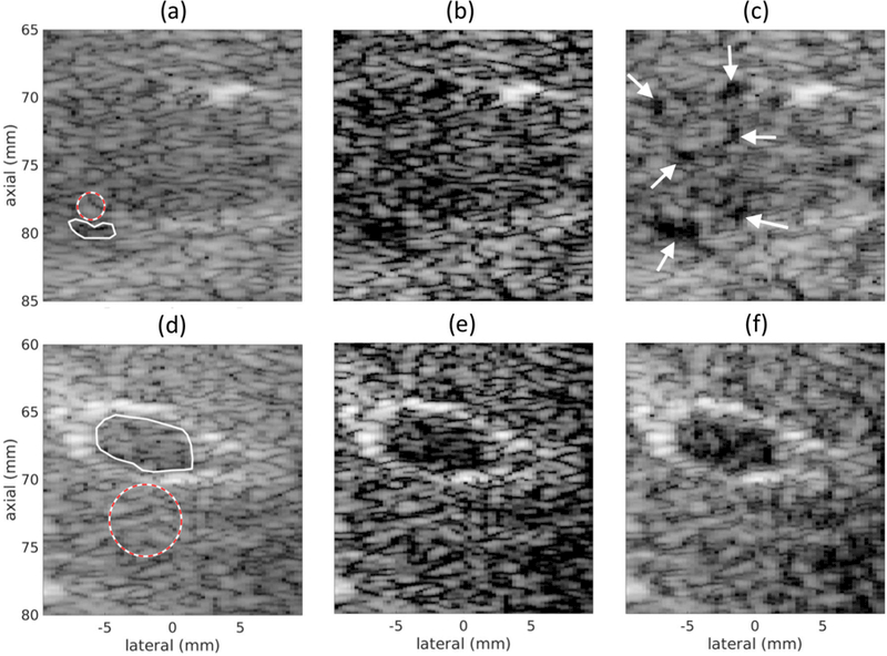
In vivo scans of human liver using (a, d) DAS, (b, e) CF, and (c, f) DNNs. The regions used to compute CR, CNR, and SNRs recorded in Table VI are shown in (a) and (d). The region with a solid line indicates the inside region and the region with a dashed line indicates the background region. Images are shown with a 60 dB dynamic range.

Table VI.

SPECKLE STATISTICS FOR IN VIVO SCANS

	Fig. 11 (a–c)			Fig. 11 (d–f)
Parameter	DAS	CF	DNN	DAS	CF	DNN
CR (dB)	6.5	20.7	25.7	1.2	8.6	9.5
CNR (dB)	−0.4	−0.3	4.5	−15.9	−5.2	−1.5
Speckle SNR	2.03	1.07	1.75	1.83	0.96	1.44

The scan in Figs. 11 (a–c) was of a region in the liver that did not contain any major blood vessels. The white arrows in Fig. 11 (c) indicate small blood vessels that were revealed by the DNN approach that were not apparent in the DAS image and only somewhat visible in the CF image. Using the regions traced by the solid and dashed lines in Fig. 11, the DNN approach improved the contrast ratio by 19.2 dB and CNR by 4.9 dB Compared to the CF, the DNN approach improved the contrast ratio by 5 dB and CNR by 4.8 dB.

The scan in Figs. 11 (d–f) was of a larger blood vessel in the liver. Compared to DAS, the DNN approach improved the contrast ratio by 8.3 dB and contrast-to-noise ratio by 14.4 dB. Compared to the CF, the DNN approach improved the contrast ratio by 0.9 dB and CNR by 3.7 dB.

F. Depth of Field

The networks trained in this work had a depth of field, which resulted in a degraded speckle pattern away from the training depth. To quantify depth of field, we simulated a speckle target phantom that was 4 cm in depth and centered at the 7 cm transmit focal depth. The images for this phantom using DAS, CF, and the DNN approach are in Fig. 12. These results show that the DNN approach increased speckle variance as the distance from the training depth increased.

Fig. 12.

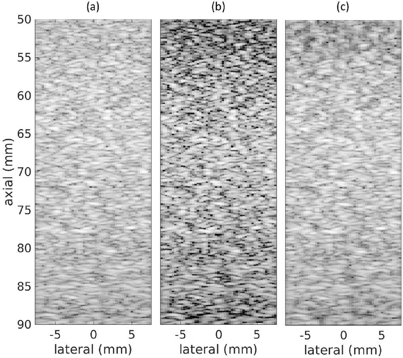
Simulated speckle target through depth using (a) DAS, (b) CF, and (c) DNNs. White Gaussian noise was added such that the channel SNR was 50 dB. Images are shown with a 60 dB dynamic range.

We computed speckle SNR as a function of depth for five realizations of the images in Fig. 12 and averaged the resulting curves. The average speckle SNR curve as a function of depth is in Fig. 13, which shows that speckle SNR was fairly constant when using DAS but decreased away from the focus when using the DNN approach and the CF. Using a criterion of 10% difference between the DNN speckle SNR values and the theoretical value for the SNR of a Rayleigh distribution, the depth of field for the DNN approach was 2.6 cm. For the CF, the degradation in speckle SNR was at least 25% and increased as a function of the distance from the transmit focal depth.

Fig. 13.

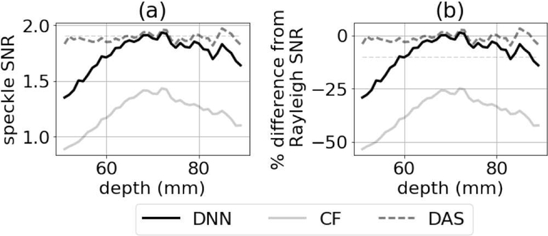
(a) Speckle SNR as a function of depth for standard DAS and DNN approach. (b) Percent difference between speckle SNR for DAS, CF, and DNNs relative to the theoretical speckle SNR assuming a Rayleigh distribution. A 10% difference criterion is indicated as a dashed line and was used to determine the depth of field for the DNN approach.

G. Revealing Network Operation

One of the criticisms of using neural networks is that direct examination of a network architecture with its parameter weights does not provide insight into how a network performs the task that it was trained to do. We examined several methods for illuminating how the networks trained in this work accomplish the task they were trained to perform.

1) Fixed Network Response:

In the first network examination method, the network for the transmit frequency was provided signals from the acceptance or rejection region. As a particular input signal was propagated through the network, we kept track of the neurons that became active. Those neurons that did not become active were removed from the network along with all of their connections. The activation functions of the active neurons were also replaced with linear functions. In essence, we fixed the network based on a specific input signal. Next, this linearized and fixed network was exposed to point target responses from a grid of points located along the center of the annular sector shown in Fig. 5 and a beam profile plot was created.

The beam profile plots for adaptive (no network alterations) and fixed network and for several kinds of inputs used to fix the network are in Fig. 14. In Fig. 14 (a), the network was fixed based on an on-axis point target (i.e., an acceptance region signal). The result shows that the fixed response resembled the response when using DAS. In Fig. 14 (b), the network was fixed based on a signal from a region of background speckle. In this case, the fixed response also resembled the response when using DAS. In Fig. 14 (c), the network was fixed based on a signal originating from the center of an anechoic cyst. The result shows that the fixed response was a beam that had a similar shape to DAS, but attenuated all signals by at least 80 dB.

Fig. 14.

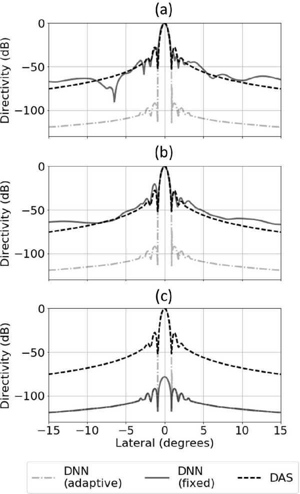
Adaptive network and fixed network responses for (a) center of point target, (b) area of diffuse scattering, and (c) middle of an anechoic cyst. The fixed and adaptive DNN responses were normalized with respect to the DAS response. These beam profiles are for the transmit center frequency.

The results from this analysis show that the network adjusted the beam based on the type of signal was at the input. In the case of the main lobe point scatter and speckle region target, the fixed response resembled the standard DAS response and the network seemed to act like a normal beam. In contrast, when the network was fixed using a signal from the center of a cyst, the network created a beam that attenuated both main lobe and side lobe signals by about 80 dB relative to DAS.

The fixed response from the main lobe point target in Fig. 14 (a) also showed the presence of a deep null in the beam profile. This null is similar to those observed when examining the beams produced by minimum variance beamforming [15]. Similar to minimum variance, it is possible the network learned how to place nulls at specific locations to suppress areas of strong off-axis scattering. For comparison, examples of minimum variance weights and associated beam profiles are in Fig. 17.

Fig. 17.

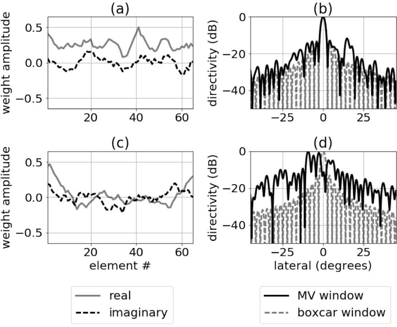
Complex apodization weights computed using minimum variance beamforming are in the left column for (a) an anechoic cyst and (c) a region of diffuse scattering. Corresponding beam profiles are in the right column.

2) Neuron Activity:

The second method that we examined for revealing network function was to compute the fraction of active neurons as a function of the hidden layer number. Similar to looking at fixed network responses, we propagated different kinds of input signals through the network and monitored the fraction of active neurons as a function of hidden layer. The results from this analysis are in Fig. 15.

Fig. 15.

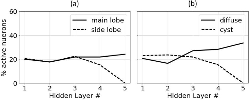
Percent of active neurons for (a) point target responses and (b) diffuse scattering responses.

Fig. 15 (a) shows the results for this analysis for the signal from an on-axis point target and for the signal from a point target in the side lobe region of the beam. Fig. 15 (b) shows the results of this analysis for a signal originating from a region of background speckle and for a signal originating from the middle of an anechoic cyst.

The results in Fig. 15 show that for the examined signals, a limited number of the total neurons in the network became active as the signals propagated through the network. In general, approximately 20–40% of the neurons became active. In addition, these results show that the network suppressed rejection region signals by reducing the activation rate of the neurons in the final hidden layers such that the last hidden layer contained no active neurons when the network was exposed to a rejection region signal.

3) First Layer Apodization:

The last method we used to analyze network function was to compute beam profiles for the complex apodization weights applied to the first hidden layer of the networks. The results from this analysis are in Fig. 16 and show the different kinds of beams that the network learned for several of the neurons in the first hidden layer. The complex weights in the first layer do not look dissimilar to the weights computed using a minimum variance beamformer. The distribution of deep nulls also has some similarities to minimum variance beamforming [15]. For comparison, examples of minimum variance weights and associated beam profiles are in Fig. 17.

Fig. 16.

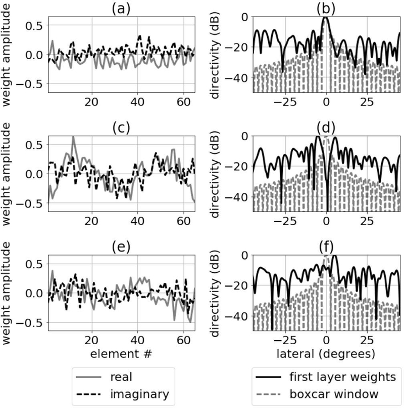
Complex apodization weights are in the left column. Corresponding beam profiles are in the right column. The results are shown for three of the nodes in the first hidden layer.

IV. DISCUSSION

The simulated anechoic cyst results in Section III-C showed that the DNN approach improved contrast ratio and contrast to-noise ratio. During training and evaluation, the network was only shown the responses from individual point targets. The signals inside the cyst region were the combined responses of many point targets in the rejection region for the network and the results show that the network learned to suppress these signals. The signals from a background speckle region were also the combined responses from many point targets and the results indicated that the network learned to not suppress these signals. One would expect diffuse scattering signals like these to be far outside the signal space in which the networks were trained, and it would not have been surprising if the networks did not generalize to these new areas of the aperture domain signal space. But the results presented in this section showed that the network generalized to diffuse scattering signals in such a way as to improve image contrast while preserving speckle. This result suggests that the networks may be behaving linearly in terms of summation.

The physical phantom anechoic cyst results in Section III-D showed that networks trained using simulated training data provided improvements to CR and CNR, while causing small decreases in speckle SNR. It seems feasible that if the training data could be better matched to physical reality by using more representative simulations or even creating training data using experiments, the speckle variance of the DNN approach could be decreased and made to be similar to DAS. It may also be important to introduce sound speed errors and other sources of degradation into the training process. Doing so could boost the image quality improvements offered by the DNN approach to in vivo scans.

The selected network used a dropout probability of 4.4×10⁻⁴. In addition, we report the validation loss as a function of dropout in Fig. 7 (a), which shows a positive correlation between dropout and validation loss. This finding suggests that for the multivariate regression problem studied in this work the disadvantages of dropout may outweigh the advantages. We hypothesize that the layers of the network can be divided into two stages: the first stage solves a classification problem (i.e., does the signal contain clutter components or not) and the second stage reconstructs the signal using only non-clutter components. If this is the case, it may be useful to include dropout in the classifier stage and to only remove dropout from the reconstruction stage.

The results from the anechoic cyst phantom experiment in Fig. 10 suggest that the networks trained in this work are robust to noise and have noise suppressing ability. The character of the envelope inside the physical phantom cyst is that of noisy data and the network successfully suppressed this noisy data inside the cyst.

The in vivo result in Fig. 11 (c) demonstrated how the DNN approach revealed small blood vessels that were not apparent in the standard DAS image. The regions with reduced image intensity contained aperture domain signals that were in the suppression region of signal space for the networks. These signals were suppressed because they were actually clutter in the form of off-axis scattering or because of model mismatch between training and physical reality or the presence of sources of acoustic clutter not accounted for during training (e.g., reverberation). Introducing other sources of image degradation to the training data will increase confidence that the revealed structures are due to the former.

The CF provided better contrast ratio than the DNN approach in the simulated anechoic cyst. Otherwise, the DNN approach performed better than the CF.

The depth of field analysis in Section III-F demonstrated that the networks trained in this work had a depth of field of approximately 2.6 cm. Maintaining good speckle quality outside of this range would require adjusting the weights of the network using a different set of training data. It may be possible to expand the depth of field by increasing the thickness of the annular sector used to generate the original training data. Synthetic aperture methods may also expand the depth of field.

The probe properties used for the training, validation, and test data sets were identical to those used in the simulation. These properties were selected to match the probe properties for the ATL L7–4 38 mm linear array used in the experiments. Discrepancies between assumed and actual probe geometries could cause significant issues for the DNN approach. In terms of the geometry of the probe, the pitch is probably the most important parameter as it controls the spatial sampling of the array. We have not systematically studied the effect of errors between assumed and actual probe properties on the DNN approach. However, we would expect probe geometry errors on the order of 5% or more to cause a large degradation in image quality for the DNN beamformer. In general, we would envision training a set of DNNs that are matched to a specific probe geometry. In terms of the mismatch between simulation and experiment, the transmit focal depth was 7 cm, so it is a reasonable to assume that the FIELD II simulations for this depth were accurate.

In this work, we trained neural networks to suppress off-axis scattering. It should be possible to train networks to suppress other sources of acoustic clutter such as reverberation. Training data for networks to suppress acoustic reverberation could be created using simulation methods developed by Byram et al. [28].

A DNN beamforming method has several advantages over similar methods such as ADMIRE that employ non-linear processing. First, processing aperture domain data with a set of networks provides a more flexible foundational framework with faster real-time potential because the computationally expensive training phase can be performed ahead of time. Second, DNNs do not include a tuning parameter at time of execution. Finally, it may be possible to train DNNs to handle high dynamic range imaging applications such as cardiac imaging better than adaptive beamformers. Others have shown that most existing adaptive beamformers perform poorly on high dynamic range signals where clutter level is much higher than the signal of interest [29], [30]. It may be possible to train DNNs to reduce or eliminate this observed degradation.

The DNNs used in this work were fully connected feed forward neural networks. Moving toward more advanced net work architectures has helped to improve the effectiveness of neural networks in other applications and it is possible that the same gains could be realized by using more advanced network architectures for the application in this work. Con volutional networks have improved the effectiveness of neural networks in many applications; however, they assume that the important features for suppressing clutter in aperture domain signals are spatially localized, which is an assumption that is not obvious for this application. In addition, convolutional networks offer the greatest advantages to problems that have many inputs (e.g., treating each pixel in an image as an input to a network). The number of elements in a linear ultrasound array is relatively small compared to the number of pixels in an image. Convolutional networks may offer advantages when using DNNs to suppress clutter in matrix array data.

V. CONCLUSION

In this paper, we proposed a novel DNN approach for suppressing off-axis scattering. Although DNNs have been used to solve classification problems based on ultrasound B-mode images before, to our knowledge they have never been used for the purposes of ultrasound beamforming. The networks were trained using FIELD II simulated responses from individual point targets. Using the proposed method we showed improvements to image contrast in simulation, phantom experiment, and in vivo data. We also explored how the networks operated to reduce off-axis scattering by examining fixed and adaptive network responses and the number of active neurons per hidden layer. Our results demonstrate that DNNs have potential to improve ultrasound image quality.

REFERENCES

- [1].Hollman KW, Rigby KW, and O’Donnell M, “Coherence factor of speckle from a multi-row probe,” in Proc. IEEE Ultrason. Symp, 1999, vol. 2, pp. 1257–1260. [Google Scholar]
- [2].Li PC and Li ML, “Adaptive imaging using the generalized coherence factor,” IEEE Trans. Ultrason. Ferroelectr. Freq. Control, vol. 50, no. 2, pp. 128–141, 2003. [DOI] [PubMed] [Google Scholar]
- [3].Lediju MA, Trahey GE, Byram BC, and Dahl JJ, “Short-lag spatial coherence of backscattered echoes: Imaging characteristics,” IEEE Trans. Ultrason. Ferroelectr. Freq. Control, vol. 58, no. 7, pp. 1377–1388, 2011. [DOI] [PMC free article] [PubMed] [Google Scholar]
- [4].Byram B and Jakovljevic M, “Ultrasonic multipath and beamforming clutter reduction: A chirp model approach,” IEEE Trans. Ultrason. Ferroelectr. Freq. Control, vol. 61, no. 3, pp. 428–440, 2014. [DOI] [PMC free article] [PubMed] [Google Scholar]
- [5].Byram B, Dei K, Tierney J, and Dumont D, “A model and regularization scheme for ultrasonic beamforming clutter reduction,” IEEE Trans. Ultrason Ferroelectr. Freq. Control, vol. 62, no. 11, pp. 1913–1927, 2015. [DOI] [PMC free article] [PubMed] [Google Scholar]
- [6].Krizhevsky A, Sutskever I, and Hinton GE, “Imagenet classification with deep convolutional neural networks,” NIPS, 2012.
- [7].Hinton G et al. , “Deep neural networks for acoustic modeling in speech recognition: The shared views of four research groups”, IEEE Signal Process. Mag, vol. 29, no. 6, pp. 82–97, 2012. [Google Scholar]
- [8].Bordes A, Glorot X, Weston J, and Bengio Y, “Joint learning of words and meaning representations for open-text semantic parsing,” Artificial Intelligence and Statistics, pp. 127–135, 2012.
- [9].Girshick R, Donahue J, Darrell T, and Malik J, “Rich feature hierar chies for accurate object detection and semantic segmentation.” in Proc. IEEE Conf. CVPR, 2014, pp. 580–587.
- [10].Hornik K, Stinchcombe M, and White H, “Multilayer feedforward networks are universal approximators,” Neural Networks, vol. 2, no. 5, pp. 359–366, 1989. [Google Scholar]
- [11].Greenspan H, van Ginneken B, and Summers RM, “Guest editorial deep learning in medical imaging: Overview and future promise of an exciting new technique,” IEEE Trans. on Med. Imag, vol. 35, no. 5, pp. 1153–1159, 2016. [Google Scholar]
- [12].Wang G, “A perspective on deep imaging,” IEEE Access, vol. 4, pp. 8914–8924, 2016. [Google Scholar]
- [13].Gasse M, Millioz F, Roux E, Garcia D, Friboulet D, “High-quality plane wave compounding using convolutional neural networks,” IEEE Trans. Ultrason. Ferroelectr. Freq. Control, vol. 64, no. 10, pp. 1637–39, 2017. [DOI] [PubMed] [Google Scholar]
- [14].Luchies A and Byram B, “Deep neural networks for ultrasound beamforming,” in Proc. of IEEE Ultrason. Symp, 2017. [DOI] [PMC free article] [PubMed]
- [15].Holfort IK, Gran F, and Jensen JA, “Broadband minimum variance beamforming for ultrasound imaging,” IEEE Trans. Ultrason. Ferroelectr. Freq. Control, vol. 56, no. 2, pp. 314–325, 2009. [DOI] [PubMed] [Google Scholar]
- [16].Shin J and Huang L, “Spatial prediction filtering of acoustic clutter and random noise in medical ultrasound imaging,” IEEE Trans. Med. Imag, vol. 36, no. 2, pp. 396–406, 2017. [DOI] [PubMed] [Google Scholar]
- [17].Yang B, “A study of inverse short-time Fourier transform,” in IEEE Int. Conf. Acoustics, Speech and Signal Processing, 2008, pp. 3541–3544.
- [18].Kingma D and Ba J, “Adam: A method for stochastic optimization,” in ICLR, 2015.
- [19].Chollet F et al. “Keras,” 2015. [Online]. Available: https://github.com/fchollet/keras.
- [20].Abadi M et al. , “TensorFlow: Large-Scale Machine Learning on Heterogeneous Systems,” 2015. [Online]. Available: http://tensorflow.org/about/bib.
- [21].He K, Zhang X, Ren S, and Sun J, “Delving deep into rectifiers: Surpassing human-level performance on imagenet classification,” in Proc. IEEE ICCV, pp. 1026–1034, 2015.
- [22].Clevert D, Unterthiner T, and Hochreiter S, “Fast and accurate deep network learning by exponential linear units (ELUs),” in ICLR, 2015.
- [23].Goodfellow I, Bengio Y, and Courville A. Deep learning MIT press, 2016. [Google Scholar]
- [24].Srivastava N, Hinton GE, Krizhevsky A, Sutskever I, and Salakhut dinov R, “Dropout: a simple way to prevent neural networks from overfitting,” Journal of Machine Learning Research, vol. 15, no. 1, pp. 1929–1958, 2014. [Google Scholar]
- [25].Stanford University CS231n: Convolutional Neural Networks for Visual Recognition, “Neural Networks Part 2: Setting up the Data and the Loss,” 2017. [Online]. Available: http://cs231n.github.io/neural-networks-2. [Accessed: 20- Dec- 2017].
- [26].Jensen JA and Svendsen NB, “Calculation of pressure fields from arbitrarily shaped, apodized, and excited ultrasound transducers,” IEEE Trans. Ultrason., Ferroelec., Freq. Contr, vol. 39, pp. 262–267, 1992. [DOI] [PubMed] [Google Scholar]
- [27].Choromanska A, Henaff M, Mathieu M, Arous GB, and LeCun Y, “The Loss Surfaces of Multilayer Networks,” in PMLR, 2015, pp. 192–204.
- [28].Byram B and Shu J, “A pseudo non-linear method for fast simulations of ultrasonic reverberation,” in SPIE Medical Imaging, 2016.
- [29].Rindal O, Rodriguez-Molares A, and Austeng A, “The dark region artifact in adaptive ultrasound beamforming,” in Proc. IEEE Ultrason. Symp, 2017.
- [30].Dei K, Luchies A, and Byram B, “Contrast ratio dynamic range: A new beamformer performance metric,” in Proc. IEEE Ultrason. Symp, 2017.