Role of Dimensionality in Predicting the Spontaneous Behavior of the Brain Using the Classical Ising Model and the Ising Model Implemented on a Structural Connectome

Abstract

There is accumulating evidence that spontaneous fluctuations of the brain are sustained by a structural architecture of axonal fiber bundles. Various models have been used to investigate this structure–function relationship. In this work, we implemented the Ising model using the number of fibers between each pair of brain regions as input. The output of the Ising model simulations on a structural connectome was then compared with empirical functional connectivity data. A simpler two-dimensional classical Ising model was used as the baseline model for comparison purpose. Thermodynamic properties, such as the magnetic susceptibility and the specific heat, illustrated a phase transition from an ordered phase to a disordered phase at the critical temperature. Despite the differences between the two models, the lattice Ising model and the Ising model implemented on a structural connectome (the generalized Ising model) exhibited similar patterns of global properties. To study the behavior of the generalized Ising model around criticality, calculation of the dimensionality and critical exponents was performed for the first time, by introducing a new concept of distance based on structural connectivity. Same value inside the fitting error was found for the dimensionality in both models suggesting similar behavior of the models around criticality.

Introduction

The relationship between the spontaneous activity of the brain and its structural fiber distribution is a critical topic in neuroscience. This relationship will allow us to better understand the emergence of complex but flexible dynamics (brain functions) in the brain from its underlying structural network. The structure–function relationship is commonly investigated using two main approaches. First, statistical methods directly compare resting-state functional connectivity patterns with the structure. Statistical comparisons lead to important results indicating the presence of a significant correlation between anatomical fiber distribution and functional connectivity patterns (Barttfeld et al., 2015; Liégeois et al., 2015; Van Den et al., 2010). The other common approach to understand the structure–function relationship of the brain is by using simple mathematical models that could capture the complex dynamics of the brain.

There are several models that have been used to discuss the spontaneous behavior of the brain, including the Neural mass model, the Kuramoto model, and the well-known two-dimensional (2D) classical Ising model. The Neural mass model and the Kuramoto model have been successful in providing evidence for the existence of a connection between the anatomical structure and the spontaneous fluctuations of the brain as captured by functional Magnetic Resonance Imaging (fMRI) (Acebrón et al., 2005; Breakspear et al., 2010; David et al., 2004; Deco et al., 2009; Honey et al., 2009).

The classical Ising model was developed by Ernest Ising (Brush, 1967) to explain the phase transition to ferromagnetic behavior at a critical temperature. It has been used to investigate brain dynamics by Fraiman et al. (2009). The classical Ising model is a relatively simple model with only one fitting parameter, the temperature of the thermal bath, in which a lattice simulating the regions of a ferromagnet is immersed. Yet, by virtue of its simplicity it has been able to capture the integration and segregation behavior of spontaneous brain function (Fraiman et al., 2009) (for more details of the 2D classical Ising model, see Supplementary Appendix A; Supplementary Data are available online at www.liebertpub.com/brain). Blood oxygen-level-dependent (BOLD) signal is the signal that fMRI methods are sensitive to and a convolved property of neuronal fluctuations in the brain. It is modeled with the Ising model using binary spin states. BOLD signals greater than a threshold will be represented by up spins and less than the threshold will be represented by down spins with the lattice sites counting the number of brain regions. With this analogy, the 2D classical Ising model was first used by Fraiman to predict the distribution of functional correlations in the brain. They found that the best prediction of the distribution of correlations was obtained from the model at the critical temperature while important deviations were observed for even small changes in temperature from criticality. Successful results of these comparisons have led to further investigations of the model to explain the structure–function relationship of the brain.

In a subsequent work, the 2D classical Ising model was generalized by Marinazzo et al. (2013) by implementing the model on the structural connectome, to match each region of the brain with a corresponding lattice site. Criticality was confirmed for the generalized model and an information transfer was found to be maximum at the critical temperature as well. The generalized Ising model was further studied by Stramaglia et al. (2017) by comparing correlation values and transfer entropy between simulated and functional empirical data. Furthermore, Deco et al. (2012) studied an Ising model implemented on the structural connectome and compared with the implementations of the model on artificially created connectomes with different coupling strengths. They investigated the entropy of the systems as a function of the coupling strength to conclude that the simulated system exhibits rich dynamics similar to the empirical functional connectivity when the structure is integrated as a scale-free network.

In this article we compared the classical Ising model and the Ising model implemented on the structural connectome with respect to the empirical data demonstrating that both models exhibit similar functional patterns and global properties despite the intrinsic differences. If both models are in the same universality class (same critical exponents), then their similarity would not be surprising. To investigate the cause of their similarities, the critical exponents (explained below and in Supplementary Appendix B) of both models were calculated and compared (Landau and Kurt Binder, 2014). If we know the critical exponents of one system in a particular universality class, we can explain any other system in the same universality class, whose microscopic causes could be totally different from the known system. The critical exponents are said to explain the behavior of the system around the critical temperature. Greek letters, β, γ, α, η, and ν, are used to represent the critical exponents of magnetizations, susceptibility, specific heat, correlation function (Expert et al., 2011), and correlation length (Fraiman et al., 2012), respectively. These critical exponents together with the dimensionality d follow the scaling relationships explained in Supplementary Appendix B.

Dimensionality, together with the other critical exponents, is fundamental to understand the behavior of the system around criticality. Physiological changes of the brain, as, for example, induced by sleep, could be in fact explained by the model deviating from criticality. Dimensionality of a system has been found to be highly relevant for the system perfomance also in neural networks (Severino et al., 2016). In their article, they have concluded that different dynamics can be observed in neural networks with different connectivity patterns coming from different dimensionalities.

For the classical Ising model, the dimensionality of the system is given by the number of dimensions of the lattice (d = 2 for a square lattice) and there is a well-defined relationship between the number of nearest neighbors in the lattice and the dimensionality (number of nearest neighbors = 2 × dimensionality). However, for the generalized Ising model, the dimensionality of the system is not evident as for the classical case and to be extracted a new concept of distance needed to be introduced.

The key components of the steps carried out are summarized in Figure 1. The organization of the article is as follows. In the next section, we introduce the methodology of calculating and comparing properties of the empirical functional connectivity with the ones generated from the numerical simulations of the classical Ising model and the generalized Ising model. Then, we explain the procedure followed to calculate the critical exponents and the dimensionality of the models. Next, we explain the main findings of the work that was carried out, followed by discussion and conclusions.

FIG. 1.

Summarized representation of the analysis carried out. We obtained the structural and functional data separately from brain imaging techniques. Then, the structural connectivity was used as the input of the generalized Ising model. Using this input, the generalized Ising model was simulated for different temperatures and each time the output was compared with the empirical functional data obtained from fMRI. fMRI, functional Magnetic Resonance Imaging. Color images available online at www.liebertpub.com/brain

Materials and Methods

Acquisition and preprocessing of data

Subjects

A set of 66 healthy subjects, between 22 and 35 years, was studied during wakefulness. Informed consent to participate in the study was obtained from every subject.

Ethics statement

The Ethics Committee of the Washington University and the University of Minnesota approved the study.

Acquisition and preprocessing of data

Structural and functional data were acquired at the Washington University and the University of Minnesota Consortium of the Human Connectome Project (WU-Minn HCP). Details about data acquisition and preprocessing can be found here (Andersson et al., 2003; Andersson and Sotiropoulos, 2015a, 2015b; Fischl, 2012; Glasser and Van Essen, 2011; Glasser et al., 2013; Jenkinson et al., 2002, 2012; Van Essen et al., 2012). Parcellation of the data was performed, using FSL, Freesurfer, and MRTrix software with 84 individually labeled regions (a list of the labels is presented in Supplementary Appendix C). Extraction of the structural connectivity matrix (J_ij) was performed using the MRTrix softtware (Daducci et al., 2012).

2D Ising model and the generalized Ising model

Computer simulations

An instance of the 2D Ising model is built starting with a random spin configuration on a square lattice of size L × L ( = 9 × 9), which is in contact with a thermal bath of temperature T. For comparison purposes, a square lattice Ising model with a 9 × 9 lattice size was chosen, as it gives 81 spin sites (that is the closest number of sites to 84 we can acquire using a square lattice). For the generalized Ising model, a 1 × 84 array of random spins was used. Each spin can be in only one of two spin states (either up [+1] or down [−1]). The energy of this spin configuration, in the absence of an external magnetic field, is given as follows:

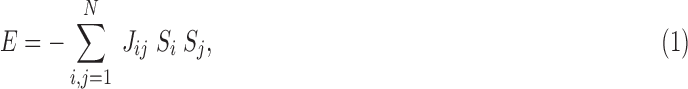where J_ij is the coupling between i^th and j^th region, s_i and s_j represent the spins of the ith and jth region, respectively, and N = L × L. A matrix representing the coupling J_ij for the 2D Ising model has been created to encode nearest neighbor coupling with a coupling strength of one (Fraiman et al., 2009). In contrast, another matrix representation of coupling J_ij for the generalized Ising model has been created using the connectivity matrix built from the diffusion tensor image (DTI) acquisition (Cammoun et al., 2012). This matrix contains the number of fiber tracts between each pair of region in the connectome used to define the coupling strength. For the simulations of the model, we normalized the average structural connectivity matrix (average over 66 subjects) such that the matrix elements will be between 0 and 1.

A Metropolis Monte Carlo algorithm (Gould et al., 1988; Metropolis et al., 1953) was used to simulate the system at each temperature. The Metropolis Monte Carlo algorithm allows to generate an equilibrium spin configuration starting from a random spin configuration for each temperature (more details can be found in Supplementary Appendix A). From the final output of the simulations, the correlation between the time evolutions of spins for each temperature was calculated using Equation (2) as follows:

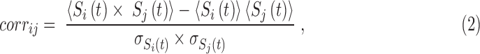where s_i and s_j stand for the spins of i^th and j^th regions, and <. > is for the average over time.

Using this procedure, the correlations were generated by each model as a function of temperature. Afterward, this procedure was repeated for both models to generate 10 sets of data for each, always starting with a random spin configuration. Generating 10 independent simulations further ensures that the Metropolis algorithm explores a variety of initial conditions and therefore increases the (statistical) accuracy of the results. MATLAB was used for computer simulations and analysis, whereas RStudio was used to generate graphs.

Analysis

Preliminary analysis

Analysis was performed over an average of 10 data sets for both models. The thermodynamic properties were plotted as functions of temperature for the two models to obtain critical temperature (Fig. 2).

FIG. 2.

Thermodynamic properties of the 2D classical Ising model with 9 × 9 lattice size and the generalized Ising model as a function of temperature. Red dashed line indicates the critical temperature and the red solid lines represent the plots after fitting the given equations to calculate the critical exponents. 2D, two dimensional. Color images available online at www.liebertpub.com/brain

The critical temperature can be obtained by locating the temperature that maximizes the magnetic susceptibility of the system (Equation (3), where χ is the magnetic susceptibility, T is the temperature, and M is the magnetization) (Landau and Kurt Binder, 2014).

The empirical functional correlation matrix built by averaging the correlation matrices across the 66 healthy subjects was compared with the simulated correlation matrices (Fig. 3) for further analysis. In addition, the distribution of the correlation for the simulated data as well as for the empirical data is plotted in Figure 4.

FIG. 3.

Correlation at four different temperatures for the classical Ising model and the generalized Ising model with the correlation of the empirical data. Color images available online at www.liebertpub.com/brain

FIG. 4.

Distribution of the correlation at four different temperatures for the classical Ising model and the generalized Ising model with the distribution of correlation of the empirical data. Color images available online at www.liebertpub.com/brain

Next, the distance between the simulated correlation distributions and the empirical correlation distribution was calculated as a function of temperature and presented in Supplementry Appendix D (I). The distance between the empirical and simulated correlation distributions is quantified using the Kolmogrove–Smirnov (KS) test statistic (Massey and Frank, 1951). To calculate the KS test statistic, empirical and the simulated correlations were plotted as cumulative plots in the same graph. Next, the maximum distance between these two plots was calculated. Temperatures that minimize this maximum distance (T_min) were obtained for individual simulations. Distribution of T_min and T_c for the generalized Ising model is presented in Figure 5.

FIG. 5.

Histogram of T_c and T_min together with the fitted distributions for the generalized Ising model in 10 independent simulations. Color images available online at www.liebertpub.com/brain

To calculate the global degree as a function of threshold, correlations were separated into positive and negative correlations. Then, the global degree was calculated for the negative and positive thresholds separately for the 2D classical Ising model and the generalized Ising model and plotted in Figure 6 together with the global degree of the empirical data (Rubinov and Sporns, 2010). Taking the individual node degree into consideration, connectivity graphs are plotted for the generalized Ising model at four different temperatures and compared with the graph of the empirical data (Fig. 7).

FIG. 6.

Average degree as a function of positive and negative thresholds for the classical Ising model and the generalized Ising model together with the average degree of the empirical correlation network. Color images available online at www.liebertpub.com/brain

FIG. 7.

Connectivity graphs for the generalized Ising model for four temperatures, and the connectivity graph of the empirical network. The size of the nodes represents the degree such that larger the size, higher the degree.

Analyzing behavior at criticality using critical exponents

The critical exponents and the dimensionality were calculated for the two models by following the procedure below. First, the critical exponents related to magnetization, susceptibility, and specific heat were calculated by fitting Equations (1)–(5) (Supplementary Appendix B) to the respective plots in Figure 2. To find η and ν, the following procedure was used:

Correlation function

First, a set of distances for both models was defined using the respective connectivity matrices. For the classical Ising model, the distances were the integers from 1 to 8, since the initial configuration was a 9 × 9 2D lattice. However, for the generalized Ising model, the distance between two regions is defined as the reciprocal of the normalized number of fibers between the two regions (d_ij = 1/J_ij). We binned the continuous distances to create a set of discrete groups. Then the correlation values between pairs at the same distance were averaged to get the average correlation as a function of distance. This calculation was performed for each temperature (Fig. 8). By fitting Equation (8) (Supplementary Appendix B) to the plot of correlation function versus distance at the critical temperature, η was calculated. By subsequently using Equation (7) to fit the correlation function at the critical temperature, a numerical value for the power of the denominator ( = d − 2 + η) was then obtained. Using this fitted value and the calculated η at T_c, the dimensionality of the classical Ising model as well as the generalized Ising model was finally extracted.

FIG. 8.

Correlation function versus distance and correlation length versus temperature for the 2D classical Ising model and the generalized Ising model. Red solid line represents plots after fitting the given equations (Supplementary Appendix B). In the top panel, the dashed line represents the correlation function at the critical temperature. Color images available online at www.liebertpub.com/brain

Correlation length

Correlation length was calculated by fitting Equation (6) (Supplementary Appendix B) to the correlation function versus the distance plot at each temperature. The correlation length was plotted as a function of temperature and fitted with Equations (9) and (10) (Supplementary Appendix B) to find ν (Fig. 8).

Results

Preliminary analysis

The mean values of critical, subcritical, and supercritical temperatures over the 10 independent trials were obtained using the susceptibility plots in Figure 2 and are reported in Table 1 together with their standard deviations. The critical temperature value of the 2D Ising model agrees with the theoritical critical temperature described in Landau and Binder (2014) for the lattice size L = 9. In the generalized Ising model, the phase transition occurs at a lower temperature than that of the classical Ising model.

Table 1.

Subcritical, Critical, Supercritical Temperatures and T_min of the Generalized Ising Model and the Two-Dimensional Classical Ising Model

Model	T < Tc	T = Tmin	T = Tc	T > Tc
Generalized Ising model	0.78 ± 0.02	1.21 ± 0.04	1.39 ± 0.02	1.98 ± 0.02
Classical Ising model	1.55 ± 0.10	2.53 ± 0.20	2.55 ± 0.10	3.55 ± 0.10

Correlations for four different temperatures are presented in Figure 3. At T_c, the spatial pattern of the correlations in the generalized Ising model holds a similar spatial pattern to that of the empirical data. Distributions of the correlations for the selected four temperatures are plotted in Figure 4 along with the empirical data. For the classical Ising model, correlation distributions showed the difference between empirical distribution and the simulated one at criticality, even if the critical temperature T_c or the slightly different value T_min gave a much better prediction with respect to sub- or supercritical behavior. For the generalized Ising model, the distribution of correlations at T_c and T_min and the distribution of correlations for the empirical data were not signifantly different (p = 0.98), while the distributions at sub- and supercritical temperatures were quite distant from the empirical distribution.

According to Figure 5, the variation of T_c (and T_min) is resulted due to the randomness of the initial spin configuration in the simulations. To illustrate the intersubject variance of T_c (and T_min), distributions of T_c (and T_min) are presented in Supplementary Appendix D (II). A two-sample t-test was performed to compare the T_min values with the T_c values in individual simulations. Results of the t-test together with Figure 5 concluded that T_min and T_c are significantly different for the generalized Ising model (p < 0.001) but not significantly different for the 2D Ising model (with p = 0.4).

Graph theoretical analysis

In Figure 6, the global degree of the graphs was plotted as a function of negative and positive thresholds for both models. As observed in Figure 4, there are no negative correlations at T_c or at T_min for the classical Ising model. Therefore, in Figure 6, the degree cannot be plotted for the negative thresholds at T_c and at T_min for the classical Ising model. Figure 7 represents the functional connectivity graphs for the data obtained from the generalized Ising model simulations at subcritical, critical, and supercritical temperatures and T_min along with the connectivity graph of the empirical data. In these graphs, each point represents a brain region. It is evident that the connectivity in the network grows as the temperature goes from T < T_c to T_c and again reduced from T_c to T > T_c, and shows similar patterns for T_c and T_min.

Analyzing behavior at criticality using critical exponents

Figure 8 represents the correlation function and the correlation length plotted for the two models. These two plots were used to find the critical exponent η and the dimensionality “d” of the models. The calculation of dimensionality for the classical Ising model confirmed the expected value of 2 (since we chose the square lattice Ising model in two dimensions) giving the value of 1.93 ± 0.59. The dimensionality of the generalized Ising model was calculated for the first time giving a value of 1.92 ± 0.12 and proven equal to the classical Ising model value inside the fitting error. All the other critical exponents are reported in Table 2 together with the dimensionality for both models.

Table 2.

Critical Exponents and the Dimensionality of the Two-Dimensional Classical Ising Model and the Generalized Ising Model

Critical exponent	2D classical Ising model	Generalized Ising model
α (Specific heat)	1.49 ± 0.02	0.81 ± 0.01
β (Magnetization)	0.14 ± 0.01	0.21 ± 0.01
γ (Susceptibility)	0.61 ± 0.01	0.53 ± 0.01
η (Correlation function)	0.34 ± 0.01	0.46 ± 0.01
ν (Correlation length)	0.30 ± 0.01	0.63 ± 0.02
d (Dimensionality)	1.93 ± 0.59	1.92 ± 0.12

2D, two dimensional.

Discussion

The square lattice Ising model has been used in neuroscience to study brain functionality. Fraiman et al. showed that the distribution of correlations at T_c in the 2D classical Ising model has noticeable similarities to the distribution of correlations of the empirical data, even in the absence of information from the structural architecture of the brain (Fraiman et al., 2009). Their conclusion together with several other studies supported the assumption of the presence of critical behavior in the brain network (Deco et al., 2012; Marinazzo et al., 2013; Stramaglia et al., 2017).

In this article, as the first step we compared simulations of a 2D Ising model with those of the generalized Ising model by looking at the distibutions of correlation values. The fact that for both models the mean of correlation distribution values at the critical temperature is larger than the mean of the correlation distribution at subcritical or supercritical temperatures is a well-known prediction of the Ising model in the classical version and was confirmed by our results for the generalized model. Correlation between the i^th and j^th regions can be calculated using Equation (4) (where r_ij is the distance between region i and j, ξ is the correlation length, d is the dimensionality, and η is the critical exponent of the correlation function), and is clearly shown in Figure 8.

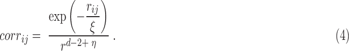At the critical temperature, because the correlation length (ξ) goes to infinity (in the infinite lattice size limit), the correlation will have a power low decay with the distance. On the contrary, at any other temperature, ξ will be finite and the correlation will have a combined exponential and power low decay. Therefore, outside of criticality, correlation will drop faster with distance resulting in a lower average correlation value. For finite lattice size, the difference between the mean of the distribution at criticality and outside criticality will be reduced with respect to the infinite lattice size limit.

In the generalized Ising model, the introduction of the coupling from the structural connectivity of the brain provided a one to one relationship between the brain regions and the lattice sites. Each lattice site was connected with every other site with a given weight obtained from DTI as opposed to the 2D classical Ising model. One objective was to investigate behavior at the critical temperature with respect to these changes in the model. When the structure is introduced, we observed a shift in the critical temperature from 2.5 to 1.4. An illustration of this change as a function of sparsity of the structural connectivity matrix is presented in Supplementary Appendix D (III). We can conclude that the critical temperature depends not only on the size of the matrix but also on the sparsity of the connectivity matrix.

The temperature that minimizes the distance between the distributions of correlation (T_min) was significantly different from T_c for the generalized Ising model but not for the 2D classical Ising model. Global degree plotted as a function of the temperature (Supplementary Appendix D (IV)) was maximized at a temperature not different from T_min. This fact suggests the usage of graph properties to extract T_min of the Ising model, either in the classical or generalized version as done by looking for the maximum susceptibility. Figure 9 represents the possibility of finding a relationship between the graph properties and the thermodynamic properties of the Ising model. As the theory implies, the specific heat and the susceptibility measure the variation of energy and magnetization with temperature, respectively. This was captured by calculating the cumulative integral of the specific heat and susceptibility of the generalized Ising model. Following the same procedure, the cumulative integral of the global degree was calculated, which resulted in the plot on the right-hand corner in the top panel of Figure 9. The new plotted quantity follows a similar behavior as the energy with temperature and could be linked to a fundamental property of graph theory.

FIG. 9.

Energy, specific heat, magnetization, susceptibility, degree, and the cumulative degree of (a) the generalized Ising model and (b) the 2D classical Ising model as a function of temperature.

Similar properties around criticality for both models justified the use of the same fitting functions, even if we needed to introduce a concept of distance for the generalized version to extract the correlation length. In fact, as shown in Figure 8, the behavior of the correlation versus distance for the generalized Ising model is well fitted by the same function as the classical model.

Having the same dimensionality can explain the observed similarities in global behavior of the two Ising models around the critical temperature such as the correlation values and global degree. Studying the behavior around criticality for complex systems such as the Ising model, which shows a phase transition, could be extremely important and performed with a similar strategy as the one followed in this article by introducing an artificial concept of distance.

As the critical exponents (in Table 2) are different for the two models, it cannot be concluded that these models belong to the same universality class. The fact that the global properties of the models still followed a similar pattern is due to the fact that our calculated properties all depend on the correlation values controlled by the dimensionality d (equal in the two models) and the critical exponent η (0.34 for classical and 0.46 for generalized) (Supplementary Appendix B; Equation (6)).

Our findings for the generalized Ising model could be of relevance to study, for example, the brain function of patients who suffer severe brain injury with disorders of consciousness in which usually both structural and functional connectivity are highly affected (Demertzi et al., 2014). Furthermore, for future studies, it will be highly relevant to see how the properties of the generalized Ising model change with respect to the size of the lattice. This would mean using different parcellation schemes, different size of the system, contrary to the classical Ising model, will also result in the change of the structural connectivity matrix (J_ij) that will depend on the parcellation scheme used.

Conclusion

Extending the 2D classical Ising model toward the generalized Ising model further permits to fit the empirical functional connectivity patterns. The introduction of structural data from the brain as an input into the Ising model gives the best fit to functional data at T_min, which is significantly different from T_c in the direction of the subcritical region but not far from criticality. Since the critical exponents of the models are different, it cannot be concluded that these two models belong to the same universality class. However, similarities observed in the global properties between the two models can be explained by the fact that they have the same dimensionality. Studying the behavior of the system around criticality could be used to better understand changes in spontaneous brain activity from the awake condition as observed in physiological states such as sleep or as in pharmacologically induced conditions such as under anesthetics.

Acknowledgments

The authors acknowledge the Human Connectome Project (HCP) for providing the data. In particular, the data were provided by the HCP, WU-Minn Consortium (Principal Investigators: David Van Essen and Kamil Ugurbil; 1U54MH091657) funded by the 16 NIH Institutes and Centers that support the NIH Blueprint for Neuroscience Research; and by the McDonnell Center for Systems Neuroscience at Washington University. Furthermore, they also extend the acknowledgment to Marco Aiello and Carlo Cavaliere from NAPLAB, Naples (Italy), for performing the parcellation of the preprocessed HCP data and for the extraction of the structural connectivity matrix from the DTI data.

Author Disclosure Statement

No competing financial interests exist.

References

- Acebrón JA, Bonilla LL, Vicente CJP, Ritort F, Spigler R. 2005. The Kuramoto model: a simple paradigm for synchronization phenomena. Rev Modern Phys 77:137 [Google Scholar]
- Andersson JL, Skare S, Ashburner J. 2003. How to correct susceptibility distortions in spin-echo echo-planar images: application to diffusion tensor imaging. Neuroimage 20:870–888 [DOI] [PubMed] [Google Scholar]
- Andersson JL, Sotiropoulos SN. 2015a. An integrated approach to correction for off-resonance effects and subject movement in diffusion MR imaging. Neuroimage 125:1063–1078 [DOI] [PMC free article] [PubMed] [Google Scholar]
- Andersson JL, Sotiropoulos SN. 2015b. Non-parametric representation and prediction of single- and multi-shell diffusion-weighted MRI data using Gaussian processes. Neuroimage 122:166–176 [DOI] [PMC free article] [PubMed] [Google Scholar]
- Barttfeld P, Uhrig L, Sitt JD, Sigman M, Jarraya B, Dehaene S. 2015. Signature of consciousness in the dynamics of resting-state brain activity. Proc Natl Acad Sci 112:887–892 [DOI] [PMC free article] [PubMed] [Google Scholar]
- Breakspear M, Heitmann S, Daffertshofer A. 2010. Generative models of cortical oscillations: neurobiological implications of the Kuramoto model. Front Hum Neurosci 4:190. [DOI] [PMC free article] [PubMed] [Google Scholar]
- Brush SG. 1967. History of the Lenz-Ising model. Rev Modern Phys 39:883 [Google Scholar]
- Cammoun L, Gigandet X, Meskaldji D, Thiran JP, Sporns O, Do KQ, et al. 2012. Mapping the human connectome at multiple scales with diffusion spectrum MRI. J Neurosci Methods 203:386–397 [DOI] [PubMed] [Google Scholar]
- Daducci A, Gerhard S, Griffa A, Lemkaddem A, Cammoun L, Gigandet X, et al. 2012. The connectome mapper: an open-source processing pipeline to map connectomes with MRI. PLoS One 7:e48121. [DOI] [PMC free article] [PubMed] [Google Scholar]
- David O, Cosmelli D, Friston KJ. 2004. Evaluation of different measures of functional connectivity using a neural mass model. Neuroimage 21:659–673 [DOI] [PubMed] [Google Scholar]
- Deco G, Jirsa V, McIntosh AR, Sporns O, Kötter R. 2009. Key role of coupling, delay, and noise in resting brain fluctuations. Proc Natl Acad Sci 106:10302–10307 [DOI] [PMC free article] [PubMed] [Google Scholar]
- Deco G, Senden M, Jirsa V. 2012. How anatomy shapes dynamics: a semi-analytical study of the brain at rest by a simple spin model. Front Comput Neurosci 6:68. [DOI] [PMC free article] [PubMed] [Google Scholar]
- Demertzi A, Gómez F, Crone JS, Vanhaudenhuyse A, Tshibanda L, Noirhomme Q, et al. 2014. Multiple fMRI system-level baseline connectivity is disrupted in patients with consciousness alterations. Cortex 52:35–46 [DOI] [PubMed] [Google Scholar]
- Expert P, Lambiotte R, Chialvo DR, Christensen K, Jensen HJ, Sharp DJ, et al. 2011. Self-similar correlation function in brain resting-state functional magnetic resonance imaging. J R Soc Interf 8:472–479 [DOI] [PMC free article] [PubMed] [Google Scholar]
- Fischl B. 2012. FreeSurfer. Neuroimage 62:774–781 [DOI] [PMC free article] [PubMed] [Google Scholar]
- Fraiman D, Balenzuela P, Foss J, Chialvo DR. 2009. Ising-like dynamics in large-scale functional brain networks. Phys Rev E 79:061922. [DOI] [PMC free article] [PubMed] [Google Scholar]
- Fraiman D, Chialvo DR. 2012. What kind of noise is brain noise: anomalous scaling behavior of the resting brain activity fluctuations. Front Physiol 3:307. [DOI] [PMC free article] [PubMed] [Google Scholar]
- Gerhard S, Daducci A, Lemkaddem A, Meuli R, Thiran JP, Hagmann P. 2011. The connectome viewer toolkit: an open source framework to manage, analyze, and visualize connectomes. Front Neuroinf 5. [DOI] [PMC free article] [PubMed] [Google Scholar]
- Glasser MF, Sotiropoulos SN, Wilson JA, Coalson TS, Fischl B, Andersson JL, et al. 2013. The minimal preprocessing pipelines for the Human Connectome Project. Neuroimage 80:105–124 [DOI] [PMC free article] [PubMed] [Google Scholar]
- Glasser MF, Van Essen DC. 2011. Mapping human cortical areas in vivo based on myelin content as revealed by T1- and T2-weighted MRI. J Neurosci 31:11597–11616 [DOI] [PMC free article] [PubMed] [Google Scholar]
- Gorgolewski K, Burns CD, Madison C, Clark D, Halchenko YO, Waskom ML, et al. 2011. Nipype: a flexible, lightweight and extensible neuroimaging data processing framework in python. Front Neuroinf 5. [DOI] [PMC free article] [PubMed] [Google Scholar]
- Gould H, Tobochnik J, Meredith DC, Koonin SE, McKay SR, Christian W. 1996. An introduction to computer simulation methods: applications to physical systems. Comput Phys 10:349 [Google Scholar]
- Honey C, Sporns O, Cammoun L, Gigandet X, Thiran JP, Meuli R, et al. 2009. Predicting human resting-state functional connectivity from structural connectivity. Proc Natl Acad Sci 106:2035–2040 [DOI] [PMC free article] [PubMed] [Google Scholar]
- Jenkinson M, Bannister PR, Brady JM, Smith SM. 2002. Improved optimisation for the robust and accurate linear registration and motion correction of brain images. NeuroImage 17:825–841 [DOI] [PubMed] [Google Scholar]
- Jenkinson M, Beckmann CF, Behrens TE, Woolrich MW, Smith SM. 2012. FSL. Neuroimage 62:782–790 [DOI] [PubMed] [Google Scholar]
- Landau DP, Binder K. 2014. A Guide to Monte Carlo Simulations in Statistical Physics. New York, NY: Cambridge University Press, pp. 13–22 [Google Scholar]
- Liégeois R, Ziegler E, Phillips C, Geurts P, Gómez F, Bahri MA, et al. 2015. Cerebral functional connectivity periodically (de) synchronizes with anatomical constraints. Brain Struct Funct 221:1–13 [DOI] [PubMed] [Google Scholar]
- Marinazzo D, Pellicoro M, Wu GR, Angelini L, Cortes JM, Stramaglia S. 2013. Information transfer of an Ising model on a brain network. BMC Neurosci 14:123280045 [Google Scholar]
- Massey Jr FJ. 1951. The Kolmogorov-Smirnov test for goodness of fit. J Am Stat Assoc 46:68–78 [Google Scholar]
- Metropolis N, Rosenbluth AW, Rosenbluth MN, Teller AH, Teller E. 1953. Equation of state calculations by fast computing machines. J Chem Phys 21:1087–1092 [Google Scholar]
- Penny WD, Friston KJ, Ashburner JT, Kiebel SJ, Nichols TE. 2011. Statistical Parametric Mapping: The Analysis of Functional Brain Images. Cambridge, MA: Academic Press, pp. 3–49 [Google Scholar]
- Ribeiro de Paula D, Ziegler E, Abeyasinghe PM, Das TK, Cavaliere C, Aiello M, et al. 2017. A method for independent component graph analysis of resting‐state fMRI. Brain Behav 7:e00626. [DOI] [PMC free article] [PubMed] [Google Scholar]
- Rubinov M, Sporns O. 2010. Complex network measures of brain connectivity: uses and interpretations. Neuroimage 52:1059–1069 [DOI] [PubMed] [Google Scholar]
- Stramaglia S, Pellicoro M, Angelini L, Amico E, Aerts H, Cortés JM, et al. 2017. Ising model with conserved magnetization on the human connectome: implications on the relation structure-function in wakefulness and anesthesia. CHAOS 27:047407. [DOI] [PubMed] [Google Scholar]
- Tournier JD, Calamante F, Gadian DG, Connelly A. 2004. Direct estimation of the fiber orientation density function from diffusion-weighted MRI data using spherical deconvolution. Neuroimage 23:1176–1185 [DOI] [PubMed] [Google Scholar]
- Ulloa Severino FP, Ban J, Song Q, Tang M, Bianconi G, Cheng G, Torre V. 2016. The role of dimensionality in neuronal network dynamics. Sci Rep 6:29640. [DOI] [PMC free article] [PubMed] [Google Scholar]
- van den Heuvel MP, Pol HEH. 2010. Exploring the brain network: a review on resting-state fMRI functional connectivity. Eur Neuropsychopharmacol 20:519–534 [DOI] [PubMed] [Google Scholar]
- van den Heuvel MP, Sporns O. 2013. Network hubs in the human brain. Trends Cogn Sci 17:683–696 [DOI] [PubMed] [Google Scholar]
- Van Essen DC, Glasser MF, Dierker DL, Harwell J, Coalson T. 2012. Parcellations and hemispheric asymmetries of human cerebral cortex analyzed on surface-based atlases. Cereb Cortex 22:2241–2262 [DOI] [PMC free article] [PubMed] [Google Scholar]
Associated Data
This section collects any data citations, data availability statements, or supplementary materials included in this article.