High precision in protein contact prediction using fully convolutional neural networks and minimal sequence features

Abstract

Motivation

In addition to substitution frequency data from protein sequence alignments, many state-of-the-art methods for contact prediction rely on additional sources of information, or features, of protein sequences in order to predict residue–residue contacts, such as solvent accessibility, predicted secondary structure, and scores from other contact prediction methods. It is unclear how much of this information is needed to achieve state-of-the-art results. Here, we show that using deep neural network models, simple alignment statistics contain sufficient information to achieve state-of-the-art precision. Our prediction method, DeepCov, uses fully convolutional neural networks operating on amino-acid pair frequency or covariance data derived directly from sequence alignments, without using global statistical methods such as sparse inverse covariance or pseudolikelihood estimation.

Results

Comparisons against CCMpred and MetaPSICOV2 show that using pairwise covariance data calculated from raw alignments as input allows us to match or exceed the performance of both of these methods. Almost all of the achieved precision is obtained when considering relatively local windows (around 15 residues) around any member of a given residue pairing; larger window sizes have comparable performance. Assessment on a set of shallow sequence alignments (fewer than 160 effective sequences) indicates that the new method is substantially more precise than CCMpred and MetaPSICOV2 in this regime, suggesting that improved precision is attainable on smaller sequence families. Overall, the performance of DeepCov is competitive with the state of the art, and our results demonstrate that global models, which employ features from all parts of the input alignment when predicting individual contacts, are not strictly needed in order to attain precise contact predictions.

Availability and implementation

DeepCov is freely available at https://github.com/psipred/DeepCov.

Supplementary information

Supplementary data are available at Bioinformatics online.

1 Introduction

Recent successes in de novo protein structure prediction have been enabled by the availability of new methods which can infer a sufficient number of correctly predicted contacts between pairs of residues in the target sequence (Monastyrskyy et al., 2016; Ovchinnikov et al., 2016). The knowledge that specific residue pairs are spatially proximate in the three-dimensional structure greatly constrains the space of possible topologies for a predicted protein structure, making it valuable in de novo prediction settings (Kim et al., 2014; Kosciolek and Jones, 2014; Marks et al., 2011; Nugent and Jones, 2012), as well as in analogous fold recognition (Buchan and Jones, 2017b). Regardless of the eventual application, the usefulness of predicted contacts depends on their being precise with few or no false positives. Predicting contacts with high precision remains challenging, particularly for small protein families.

Residue–residue contacts are predicted from large protein sequence alignments, based on the principle that evolutionary pressures place constraints on sequence evolution. Specifically, correlations in amino acid substitution patterns at a pair of sites are indicative of the residues being in contact in the structure (Göbel et al., 1994; Taylor et al., 2013). Key difficulties in obtaining accurate contact predictions arise from the well-known issue of chaining or transitive noise (Burger and van Nimwegen, 2010), and correlations arising due to other factors (Anishchenko et al., 2017). Considerable attention has been paid to decoupling direct from indirect correlations in the literature, and the most prominent (and effective) recent approaches include Direct Coupling Analysis or DCA (Marks et al., 2011; Morcos et al., 2011; Weigt et al., 2009), pseudolikelihood maximization (Balakrishnan et al., 2011; Ekeberg et al., 2013, 2014; Kamisetty et al., 2013; Seemayer et al., 2014) and sparse inverse covariance estimation (Jones et al., 2012). Most recently, groups have focussed on using supervised machine learning (ML) techniques to combine multiple sources of information in contact prediction (Cheng and Baldi, 2007; Eickholt and Cheng, 2013; Jones et al., 2015; Michel et al., 2017; Stahl et al., 2017; Wang et al., 2017a,b; Xiong et al., 2017).

An approach commonly taken in ML-based predictors is to use large feature sets, selected on their likelihood of containing information relevant to the prediction task at hand, and to let the model training process work out which features are informative for the task. Such procedures can occasionally lead to highly redundant feature sets in that useful information for the prediction task is contained in a very small subset of the inputs. Indeed, one recent study shows that such feature sets can be simplified considerably without any loss in contact precision when a deep neural network model is used (Stahl et al., 2017). In this work, we are interested in determining an input feature set that is as simple as possible but yet contains enough information for a deep neural network model to infer contacts with precision competitive with state-of-the-art methods. Further, we evaluate the extent to which predictions generated using such features can be accurate if only local windows around a putative contacting pair are considered, without considering the whole input sequence alignment. The ability to generate predictions using variable local windows in the input is afforded by the use of fully convolutional neural network models.

Although a detailed introduction to deep learning methods is beyond the scope of this paper, we will briefly discuss convolutional neural networks, and also discuss fully convolutional architectures, which we use in this work. We show that our method, named DeepCov, achieves comparable or greater precision on average than two state-of-the-art contact prediction methods, and that it is markedly more precise than these methods on alignments with very low numbers of effective sequences.

2 Materials and methods

2.1 Convolutional and fully convolutional network models

Deep learning techniques (LeCun et al., 2015) have recently proven extremely effective in tackling challenging problems in a number of problem domains. Their power lies in their ability to learn features of data at multiple levels of abstraction, beginning from relatively simple feature sets. Methodological advances (Glorot and Bengio, 2010; Goodfellow et al., 2013; Hinton et al., 2012b; Ioffe and Szegedy, 2015; Krizhevsky et al., 2012; Rumelhart et al., 1986; Srivastava et al., 2014; Sutskever et al., 2013) including those exploiting advances in computing hardware (Raina et al., 2009; Steinkraus et al., 2005), have made it feasible to train deeper neural network models, allowing for the recognition of increasingly complex patterns and the use of much larger datasets than previously possible.

Deep learning methods have been applied to contact prediction, with some recent methods proving particularly effective (Di Lena et al., 2012; Eickholt and Cheng, 2013; Stahl et al., 2017; Wang et al., 2017a,b; Xiong et al., 2017).

Whereas ‘traditional’ neural network models (including deep neural networks) consist entirely of layers of neurons that are fully connected, individual neurons in convolutional layers receive activations from only a subset of neurons in the previous layer. Convolutional neural networks (CNNs) are especially effective in image and speech recognition tasks (e.g. Hinton et al., 2012a; Krizhevsky et al., 2012; Xiong et al., 2016), as well as other problem domains, due to their ability to detect and learn local spatial patterns in data. Spatial patterns are detected by learning convolutional filters or kernels, which are small tensors (typically 2D or 3D) of weights, usually with an additional bias term. During training, the filters are effectively swept across the input and the weights and bias are adapted to respond to local features that produce the desired output. Individual neurons in the output of a convolutional layer (collectively called the output feature map) receive the results of single placements of the convolutional filter on the input. Once a convolutional filter has been trained, an output neuron activates when a local spatial pattern in the data closely matches the pattern of the weights in the kernel. A key feature of this setup is that convolutional layers can recognize spatial features regardless of their location in the input. Multiple output feature maps (and hence kernels) can be learned in a single convolutional layer, meaning that the layer can learn to recognize a number of different spatial patterns.

Typical implementations of CNNs augment convolutional layers with fully connected layers in the later stages of the model (e.g. He et al., 2016; Krizhevsky et al., 2012). This is done as a means to aggregate and compose the features learned by the convolutional layers into output features that draw on features from all parts of the input. In contrast, fully convolutional networks (FCNs; see Shelhamer et al., 2016 and references therein) omit these fully connected layers, and the spatial locality of the learned features extends all the way to the output. Configured correctly, FCNs can take inputs of arbitrary dimensionality and produce correspondingly-sized outputs, removing the need for cropping, padding or other approaches to dealing with variable-size input (Shelhamer et al., 2016). In the case of protein contact prediction, this property is advantageous for predicting contact maps for proteins of different length.

The architecture of DeepCov is discussed in Section 2.3, but in summary, we make use of a straightforward FCN architecture to predict whole contact maps from the input data in one go. This is a different (and much more efficient) approach to that of MetaPSICOV, where each set of input features results in the prediction of a single contact and the feature window needs to be moved vertically and horizontally to allow the whole map to be predicted. FCNs have been successfully employed for contact prediction (Golkov et al., 2016; Liu et al., 2018), albeit only as post-processing for the outputs of standard covariation algorithms. The plmConv approach of Golkov et al. (2016) uses as its input features the coupling matrices output from the plmDCA method (Ekeberg et al., 2013, 2014) for each pair of amino acid residue types, and was able to outperform the original MetaPSICOV method in testing. The DeepContact approach of Liu et al. (2018) uses contact predictions from several methods, together with predicted secondary structure and solvent accessibility, among other features. Compared to this work, the feature sets used by these methods offer no interesting direct interpretation of the learned model characteristics such as the neighbourhood of transitive coupling effects around each covarying residue pair.

Overall, the DeepCov approach is similar to that of Golkov et al. (2016), however, in this study our primary focus is on whether such an expressive model, combined with relatively simple input feature sets, can be used to achieve state-of-the-art results. We discuss the input feature sets next.

2.2 Input features

Two feature sets are considered:

Pair frequencies: Pair frequency data is calculated as in MetaPSICOV (Jones et al., 2015). For each pair of columns in the input alignment, the probability of observing every pair of the 20 canonical amino acids is calculated, with gap characters considered as an additional amino acid category. Frequencies for unobserved residue pairs are estimated with a pseudocount of 1. Sequence clusters are weighted based on a 62% sequence identity clustering threshold, as done for MetaPSICOV input.

Covariance: Using marginal and pair frequencies for each pair of amino acids as described above, we calculate the covariance between every pair of residues at every pair of sites, and use these as an alternative set of input features.

For a given pair of amino acid types, pair frequencies or covariances are composed as an m × m matrix, where m is the number of columns in the sequence alignment. Considering 20 amino acid types + gap, there are 21 × 21 = 441 such matrices for a given alignment. These 441 matrices are presented (in image recognition terms) as feature channels in the input to the convolutional neural networks. Feature values from all 441 channels are used to construct individual output features in the first layer of the DeepCov neural networks. Similarly, the plmConv method (Golkov et al., 2016) uses the computed pairwise coupling matrices from plmDCA as inputs, which also have dimensions 441 × m × m.

Given the feature set, the learning task is to relate the input feature set for a given protein to its corresponding binary contact map, where two residues are deemed as being in contact if their C_β atoms (C_α in the case of glycine) are within 8 Å of each other.

2.3 FCN architectures employed in DeepCov

We compare different architectures for the FCN, but the basic layout is the same (Fig. 1). Our networks involve an input layer, a Maxout layer (Goodfellow et al., 2013) to reduce the number of input feature channels from 441 to 64, one or more 2D convolutional layers, and a final sigmoid output layer, each with batch normalization applied (Ioffe and Szegedy, 2015). The only variables in terms of network architecture are the number of intermediate convolutional layers and the size of the convolutional filters used in these layers. The Maxout layer is implemented following the method given in Goodfellow et al. (2013) for convolutional layers: first, a 2D convolutional layer with filter size 1 × 1 is used to produce 128 affine output maps (i.e. no nonlinearlity is applied). Since the filter size is 1 × 1, the resulting output maps have the same spatial dimensions as the input (m × m). Next, pairs of these affine maps are max-pooled in an element-wise fashion such that 64 output feature maps are produced, which have the same spatial dimensions as the input to the max-pooling layer (m × m). This can be termed pooling along the feature axis (in contrast to spatial pooling, which is more commonly used).

Fig. 1.

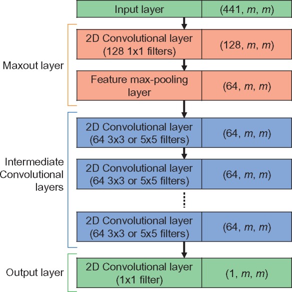
The architecture of the neural network models used for DeepCov. The number of intermediate convolutional layers and the size of the convolutional filters in these layers is variable. The three values in brackets in the right-hand cells describe the dimensionality of the data output from each layer. The values are given in the order: (number of feature channels, width, height). The width and height describe the spatial dimensions of the data and are both equal to the number of columns in the input alignment, m

The number of subsequent 2D convolutional layers is variable, but each layer is composed in a similar way: 3 × 3 or 5 × 5 filters are used (see Table 1) to generate 64 output feature maps with rectified linear unit (ReLU) activation functions. Unit stride is used, and the input feature maps to each such layer are padded with zeros such that the output feature maps have the same dimensions as the input feature maps (this is termed half- or same-padding in deep learning frameworks). This property allows us to experiment with architectures with essentially arbitrary numbers of convolutional layers. Given the locality (in feature space) of the convolution operation, having more convolutional layers effectively means that each feature in the output of the neural network can draw on information from (or ‘sees’) a larger number of features in the input. In our case, this allows us to gradually increase the size of the windows in the sequence alignment that informs the contact prediction for a given residue pair (Fig. 2).

Table 1.

Convolutional neural network architectures

Receptive field (residues)	3	5	7	9	11	13	15	17	21	25	29	33	37	41	45	49
Architecture	3	3, 3	3, 3, 3	3(×4)	3(×5)	3(×6)	3(×7)	3(×8)	5(×5)	5(×6)	5(×7)	5(×8)	5(×9)	5(×10)	5(×11)	5(×12)

Note: The architecture row lists the number of intermediate 2D convolutional layers (with their filter sizes) after the input and Maxout layers and before the final output layer, for a given receptive field size (in amino acid residues). The notation ‘5, 5, 5’ (equivalently, ‘5(×3)’) denotes three intermediate convolutional layers with filter size of 5 × 5.

Fig. 2.

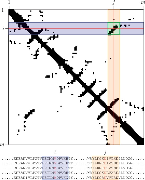
Illustration of the relationship between alignment columns and data seen by DeepCov during training and inference. Top: The receptive field of DeepCov is shown on a section of a contact map, as a highlighted square around a residue pair. The pair frequency or covariance matrices used as input to DeepCov have the same dimensions as the contact map (m × m), and DeepCov learns the relationship between the two. As the receptive field moves across the input matrix, it sees a different subset of the input, and this corresponds to a different set of columns in the input alignment (bottom). In this example, the residue pair i, j is being evaluated for the presence of a contact, and the receptive field of DeepCov is set to 11, meaning that windows of 11 residues centred on residues i and j are considered during training and prediction (shaded windows around the residues i and j in the alignment). Only the sequence data in these windows (and hence the sections in the input and output matrices covered by the receptive field) are used when learning the relationship between sequence data and the presence or absence of a contact between residues i and j

The output layer in all our networks comprises a 2D convolutional layer with a filter size of 1 × 1, a single output feature map, no zero-padding and a sigmoid activation function. This layer can be thought of as performing an aggregation over the 64 output feature maps from the previous layer, producing a single output feature map. The output from this layer has dimensions m × m and represents the predicted contact scores for all pairs of residues. Ideally, this output matrix should be symmetric, but in practice we find that it is only approximately so. Therefore, the predicted scores for residue pairs i, j and j, i are averaged to yield the final contact score for that residue pair.

Our neural network models are implemented using the Lasagne (Dieleman et al., 2015) and Theano (Al-Rfou et al., 2016) libraries for Python.

2.4 Varying receptive field size

From the point of view of a single feature in the output layer, we define the receptive field of that output feature as the size of the window around a single residue in a putative contacting residue pair which is used as the source of input features for inferring the presence or absence of a contact (see Fig. 2). As discussed above, it is possible to alter the size of the maximum possible receptive field for the network by varying the number of intermediate convolutional layers and the filter sizes used. Table 1 lists the various receptive field sizes considered, along with the setup of intermediate convolutional layers used. All intermediate convolutional layers in our networks use unit stride and half- or same-padding. Under these conditions, every intermediate layer with a filter size of k × k adds k – 1 residues to the receptive field of a single output feature (with the exception of the first intermediate layer, which adds k). For a more detailed discussion of the arithmetic of convolutional layers, we refer interested readers to Dumoulin and Visin (2016).

2.5 Training and testing

2.5.1 Protein sets for training, validation and testing

We assessed the mean precision achieved by DeepCov on the now standard PSICOV150 set of proteins and alignments, described in Jones et al. (2012). Training was carried out using a set of 6729 protein chains (chains in PDB with < 25% sequence identity and length < 500 residues). The alignments were identical to those used for training the original MetaPSICOV method (Jones et al., 2015). Proteins in the training set with any shared homologous domains with any test set protein were excluded, leaving a set of 3456 protein chains for training and validation. For validation, we arbitrarily selected the first 130 chains in PDB code alphabetical order, which is essentially a random selection. Homology between domains was assessed based on the ECOD database classification (Cheng et al., 2014).

In order to assess the performance of DeepCov on smaller protein sequence families, we constructed a second training and test set as follows. From the original set of 6729 training proteins, we selected 250 proteins whose alignments had a raw sequence count between 50 and 200 as a starting point. Chains with detectable homology to this set of 250 proteins were removed from the training set as before, leaving behind 6003 proteins. Unsurprisingly, there are far fewer homologous chains to exclude for these small families compared to the very large families in the PSICOV set. The test set was subsequently filtered to exclude proteins with fewer than five long-range contacts (sequence separation greater than 23 residues) in the native structure, leaving 232 test proteins with between 50 and 199 sequences (M_eff between 4 and 158). When evaluating the performance of MetaPSICOV2 on this dataset, the above procedure was used to construct the training set.

Additional testing was carried out on the publicly available target domains from the CASP12 experiment. For these targets, we used the alignments generated by MetaPSICOV2 during the CASP12 prediction season (Buchan and Jones, 2017a). We also compared the performance of plmConv (Golkov et al., 2016) on the 32 public CASP12 domains for which both plmConv (CASP12 group myprotein-me) and MetaPSICOV2 generated predictions during the prediction season. We used automatic evaluation results for the myprotein-me group from the Prediction Center website (predictioncenter.org), since we were unable to find plmConv itself either as a server or downloadable software. As a result, the plmConv results will have been based on a somewhat different set of alignments than MetaPSICOV2, DeepCov and CCMpred.

2.5.2 Calculation of M_eff

Alignment depth was represented both in terms of raw sequence counts, as well as the effective number of sequences (M_eff). To calculate M_eff, each alignment was clustered using CD-HIT (Fu et al., 2012; Li and Godzik, 2006) with a 62% sequence identity threshold and a word size of 4. The number of clusters returned by CD-HIT was taken as the M_eff.

2.5.3 Neural network training procedure

Training was carried out on single examples per weight update (i.e. batch size was 1), due to the size of the feature set and models, and GPU memory limits. Although a batch size of 1 is used, the batch normalization operation remains valid as the means and standard deviations are calculated across each feature map per channel. As the network is fully convolutional, variable-sized input maps can be used without any need for zero-padding or cropping of the input maps (Shelhamer et al., 2016). As an aside, the prediction of contact maps using a fully convolutional architecture is algorithmically very similar to the problem of image segmentation where input images of a particular size are transformed into output images with identical dimensions.

For initializing the weights in the networks, we used the normalized initialization procedure outlined by Glorot and Bengio (2010) with weights sampled from the uniform distribution. Network parameters were trained using the Adamax algorithm (Kingma and Ba, 2014) with early stopping (details below) to prevent overfitting. During development we found that improved results could be achieved by using stochastic gradient descent (SGD) with Nesterov momentum (Sutskever et al., 2013) and a varying learning rate, starting from the optimum found by Adamax. Both algorithms trained the network parameters by minimizing the binary cross-entropy (BCE) loss function

$$L=-t·\log p-\left(1-t\right)\log \left(1-p\right),$$

where t is the true label (presence/absence of contact represented as 1/0) and p ∈ [0, 1] is the predicted contact score for a given residue pair. The final training loss was calculated as the mean BCE across all residue pairs with a sequence separation greater than 4 residues (shorter range pairs were masked out). An L2 regularization term for the network weights was added to the BCE loss function given above, with the regularization parameter set to 10⁻⁴. When using either SGD with Nesterov momentum or Adamax, early stopping was carried out based on the Matthews correlation coefficient (MCC) between predicted and true labels on the validation set. Residue pairs with a sequence separation of 4 or fewer residues were masked out for the MCC calculation, and training was stopped when the MCC value did not improve after 10 epochs (or passes through all training examples).

Parameters for the optimizers were set as follows: the learning rate for Adamax was 0.002 and the initial learning rate for the SGD optimizer was 0.001 and the Nesterov momentum was set to 0.9. After each epoch, the SGD learning rate was incremented by a factor of 1.1 or decremented by a factor of 0.5 if the training loss decreased or increased relative to that in the previous epoch, respectively. The learning rate was not allowed to increase beyond 0.01. We found that the optimization process for any single DeepCov model typically completed training in 15–20 epochs before converging, with the longest optimization taking 30 epochs.

3 Results and discussion

We compare our method against CCMpred (Seemayer et al., 2014), a representative technique using pseudolikelihood maximization, and MetaPSICOV2, the latest version of our neural network-based contact meta-prediction approach, which was amongst the top-ranked contact prediction methods in the recent CASP12 experiment (Buchan and Jones, 2017a,b). We focus primarily on mean precision achieved for long-range contacts (sequence separation greater than 23 residues), since long-range contacts are thought to be the most informative for tertiary structure modelling (Graña et al., 2005). Some results for short-range contacts are given in the Supplementary Material.

3.1 Comparison of network architectures and feature sets

Figure 3 compares the mean precision achieved by DeepCov with differing receptive field sizes (and therefore numbers of intermediate convolutional layers) against that achieved by MetaPSICOV2 and CCMpred. In general, we find that increasing the size of the receptive field of the DeepCov model leads to gains in predictive precision on the PSICOV150 test set as expected. However, these gains tail off rapidly once a receptive field size of around 15 residues is reached; further increases in receptive field size lead to only minor gains in precision, or no clear gains in most cases. It should be pointed out that the receptive field specified by a given FCN architecture represents only a maximum possible size; the actual set of input features used to inform individual contact predictions will vary depending on the values of the trained network parameters. Nevertheless, these results suggest that a significant amount of information needed to distinguish true- from false-positive contacts can be found in reasonably close sequence proximity to the residue pair of interest.

Fig. 3.

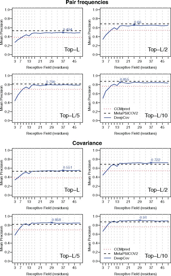
Mean long-range contact precision achieved by DeepCov on the PSICOV150 dataset using various receptive field sizes (see Table 1), using pair frequency (top 4 plots) and covariance data (bottom 4 plots). Data for DeepCov are plotted as solid lines for top-L, L/2, L/5 and L/10 predicted contacts. For DeepCov data, the maximum observed mean precision is marked. Dashed lines represent the mean precision achieved by CCMpred (dotted horizontal lines) and MetaPSICOV2 (dashed horizontal lines) respectively on the same dataset. Using covariance data, DeepCov achieves greater mean precision than CCMpred and MetaPSICOV2 when receptive field sizes of around 15 residues or more are used

Using pair frequency data as the input features (Fig. 3, top panels), DeepCov is able to almost match the average performance of MetaPSICOV2, which is quite impressive given the simplicity of the feature set. Covariance data provides higher precision than pair frequency data for a given DeepCov architecture (Fig. 3, bottom panels), and using covariance data with receptive field sizes of approximately 15 residues or greater, DeepCov outperforms both CCMpred and MetaPSICOV2 in terms of mean long-range contact precision on the PSICOV150 set of alignments. When short-range contacts are considered (Supplementary Fig. S1), DeepCov achieves similar mean precision as MetaPSICOV2, and both of these methods outperform CCMpred. The distribution of precision values for long- and short-range contacts can be found in Supplementary Figure S2.

The input feature sets used by DeepCov are conceptually much simpler than feature sets used in some other works. Many contact prediction methods (MetaPSICOV2 is one example) employ feature sets which include data such as predicted secondary structure, solvent accessibility etc., which are themselves derived from alignments; it seems that the expressive power of a sufficiently deep neural network model is able to achieve precision comparable to, and even exceeding, methods explicitly providing these ‘handcrafted’ features. Further, DeepCov does not rely on other covariation-based contact predictors. These properties present significant advantages from the end user’s perspective in that there are far fewer preprocessing steps to run (compared to MetaPSICOV2 for example). As a result, DeepCov takes considerably less time to generate predictions than MetaPSICOV2; generating new predictions using the trained neural network model takes no more than a few seconds, even on a CPU. Comparing the predicted contact scores to their true precision values (Supplementary Fig. S3), we find that DeepCov’s scores are well-calibrated and very close to their true precision on the PSICOV150 set, meaning that a priori identification of true contacts may be possible.

Comparing the true positive contacts predicted by the three methods, we find that all three methods produce a good number of unique true-positive contacts (Supplementary Fig. S4), which suggests that a metaprediction approach involving these three methods may be valuable. DeepCov produces the largest number of unique true positives. We also assessed the redundancy of the predicted contacts from a structural perspective, as done in Jones et al. (2015). We found that CCMpred tends to produce more redundant contact sets, although there is little difference between MetaPSICOV2 and DeepCov in terms of structural redundancy (Supplementary Fig. S6).

3.2 Performance on shallow alignments

Having established the superiority of the covariance-based feature set, we assessed the performance of DeepCov using covariance-based features on a set of 232 shallow alignments (see Section 2.5.1), in order to assess DeepCov’s performance on small protein families. A fixed architecture with a sufficiently large maximum receptive field of 41 residues was used (See Table 1). We find that DeepCov outperforms the other two methods in terms of the mean precision on this set of alignments (Fig. 4). Targets with relatively few sequence homologues are generally the most difficult modelling targets in the CASP experiments, and any improvements in typical precision of predicted contacts are likely to be useful. In the three ranges of M_eff in the left panel of Figure 4, DeepCov’s mean precision exceeds that of MetaPSICOV2 by 8.3, 11.9 and 17.4%, respectively. The magnitude of improvement over MetaPSICOV2 is encouraging, especially for alignments with M_eff greater than 100, as more than half of all Pfam domains of unknown structure have 100 or more effective sequences available (Michel et al., 2017). However, the median M_eff of all 232 alignments in our shallow alignment test set is 48.5, and only 26 alignments have an M_eff greater than 100. Of these, DeepCov achieves equal or greater top-L/5 precision than MetaPSICOV2 on 23 proteins, and is equal to or better than CCMpred on 25 proteins. Improvements in precision are much less pronounced when raw sequence counts are considered (right panel of Fig. 4). This is due to the well-known fact that the effective sequence number accounts for the redundancy within individual sequence families, and is thus a better predictor of ‘useful’ information content in alignments.

Fig. 4.

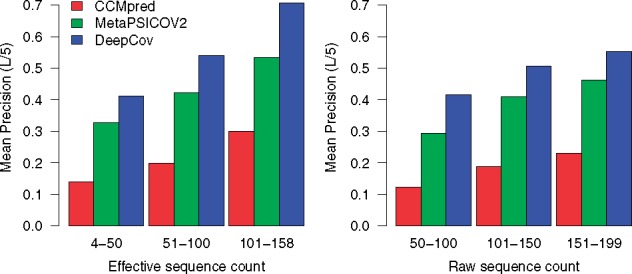
Comparison of performance on 232 shallow alignments. Mean precision for the top-L/5 contacts are plotted as a function of alignment depth for CCMpred, MetaPSICOV2 and DeepCov. Raw and effective sequence counts are binned into three categories. DeepCov achieves higher precision than CCMpred and MetaPSICOV2 on small protein sequence families. Similar trends are seen when considering the top-L, L/2 and L/10 contacts

Although DeepCov is more effective than MetaPSICOV2 and CCMpred on shallow alignments, success clearly still depends on the number of effective sequences in the input alignment, and the highest mean precision is still seen on deeper alignments. It is therefore still the case that precise contact prediction relies on having as many homologous sequences in the alignment as possible, and we hope that with further improvements to methodology, we can further lower the minimum effective alignment depth necessary to obtain predictions of sufficient quality for reliable structure modelling. As a simple test of whether contacts predicted for these shallow alignments may be useful for modelling, we considered the number of targets in each sequence bin in Figure 4 on which a precision of at least 0.5 was achieved on the top-L long-range contacts. DeepCov achieves a precision of 0.5 or higher on more targets than MetaPSICOV2 or CCMpred (Supplementary Table S1), although the fraction of such targets in each sequence bin is low. Nevertheless, these results suggest that there is room for improvement in contact precision on shallow sequence alignments, and we are currently working to improve this aspect of our methods.

3.3 Performance on CASP12 targets

Table 2 shows the performance of DeepCov on the publicly available CASP12 target domains and compares its performance to MetaPSICOV2 and CCMpred. All three methods used identical input alignments. Detailed results for each domain can be found in Supplementary Figure S5. For this analysis, we ran DeepCov with the covariance model used in Section 3.1 and a receptive field of 41 residues. It can be seen that although DeepCov does not reach MetaPSICOV2’s performance, it is remarkably precise (especially when one considers the simplicity of the input feature set), and is still considerably more precise than CCMpred.

Table 2.

Mean long-range contact precision achieved by MetaPSICOV2, DeepCov and CCMpred on the CASP12 target set

Method	Mean precision
	Top-L	Top-L/2	Top-L/5	Top-L/10
MetaPSICOV2	0.430	0.546	0.641	0.673
DeepCov	0.406	0.523	0.611	0.642
CCMpred	0.285	0.374	0.457	0.486

Note: Methods are arranged in decreasing order of mean precision.

We also compared the performance of these methods against plmConv on a common set of CASP12 domains (Section 2.5.1). We find that on this set of targets, plmConv achieves a mean L/5 precision of 53.27% on long-range contacts, whereas CCMpred, MetaPSICOV2 and DeepCov obtain mean precision values of 48.43, 67.74 and 67.99%, respectively. Again, DeepCov is competitive with MetaPSICOV2, and is much more precise than plmConv, which uses a similar FCN architecture (although plmConv used different alignments). The key difference between our approach and plmConv is the input feature set used. plmConv’s input features are the raw coupling parameters calculated by the plmDCA method, and so the input coupling matrices will already contain the predicted graphical structure of the protein. In the case of DeepCov, this structure is learned directly from the raw sequence data, across distinct protein families, and this no doubt helps our model to generalize better.

4 Conclusions

Recent work has shown that machine learning methods are proving increasingly useful for a number of challenging tasks, including protein contact prediction. In this work, we developed a contact prediction method based on fully convolutional network models but where the input features are stripped down to the absolute bare minimum of raw pairwise substitution counts derived from a multiple sequence alignment. Our results suggest that simple residue pair covariance data often contains sufficient information for predicting contacts at state-of-the-art or even higher precision. Our method is especially effective on input alignments with relatively few effective sequences. Further improvements in contact precision may be possible, for example by including DeepCov as one of the sources of contact predictions in a meta-prediction approach such as MetaPSICOV. We intend to develop the method further and look forward to testing it in upcoming CASP experiments.

Beyond the performance of the method, our results suggest that a global view of alignment statistics is not strictly necessary in order to achieve state-of-the-art results in contact prediction, provided one uses a sufficiently expressive model; even with a maximum receptive field of only 15, which would include only the 7 immediate upstream and 7 downstream residues around each of the pair of residues being considered, DeepCov reaches close to its maximum precision in our tests. It is currently not clear whether this effect is due somehow to an increased ability to disentangle correlation chains, which are assumed to be a roadblock to achieving high precision.

Correlations between residue substitutions are not necessarily indicative of intra-chain contacts; these patterns can arise due to various other factors, such as oligomerization and protein-protein interactions (Anishchenko et al., 2017; de Oliveira and Deane, 2017). An advantage of machine learning methods over approaches such as DCA is the fact that the learned models can encompass features learned across distinct sequence and structure families (Wang et al., 2017a). These advantages could translate into improved models for predicting inter-chain contacts in homo- or hetero-oligomeric complexes, as well as other biomedically relevant properties also associated with residue covariation signals.

References

- Al-Rfou R. et al. (2016) Theano: a Python framework for fast computation of mathematical expressions. arXiv e-prints 1605.02688.
- Anishchenko I. et al. (2017) Origins of coevolution between residues distant in protein 3D structures. Proc. Natl. Acad. Sci. USA, 114, 9122–9127. [DOI] [PMC free article] [PubMed] [Google Scholar]
- Balakrishnan S. et al. (2011) Learning generative models for protein fold families. Proteins Struct. Funct. Bioinf., 79, 1061–1078. [DOI] [PubMed] [Google Scholar]
- Buchan D.W.A., Jones D.T. (2017a) Contact predictions with the MetaPSICOV2 server in CASP12. Proteins Struct. Funct. Bioinf., 86, 78–83. [DOI] [PMC free article] [PubMed] [Google Scholar]
- Buchan D.W.A., Jones D.T. (2017b) EigenTHREADER: analogous protein fold recognition by efficient contact map threading. Bioinformatics, 33, 2684–2690. [DOI] [PMC free article] [PubMed] [Google Scholar]
- Burger L., van Nimwegen E. (2010) Disentangling direct from indirect co-evolution of residues in protein alignments. PLOS Comput. Biol., 6, e1000633.. [DOI] [PMC free article] [PubMed] [Google Scholar]
- Cheng H. et al. (2014) ECOD: an Evolutionary Classification of Protein Domains. PLOS Comput. Biol., 10, e1003926. [DOI] [PMC free article] [PubMed] [Google Scholar]
- Cheng J., Baldi P. (2007) Improved residue contact prediction using support vector machines and a large feature set. BMC Bioinformatics, 8, 113.. [DOI] [PMC free article] [PubMed] [Google Scholar]
- de Oliveira S., Deane C. (2017) Co-evolution techniques are reshaping the way we do structural bioinformatics. F1000Research, 6, 1224.. [DOI] [PMC free article] [PubMed] [Google Scholar]
- Di Lena P. et al. (2012) Deep architectures for protein contact map prediction. Bioinformatics, 28, 2449–2457. [DOI] [PMC free article] [PubMed] [Google Scholar]
- Dieleman S. et al. (2015) Lasagne: first release. In: Zenodo. doi:10.5281/zenodo.27878.
- Dumoulin V., Visin F. (2016) A guide to convolution arithmetic for deep learning. arXiv e-prints 1603.07285.
- Eickholt J., Cheng J. (2013) A study and benchmark of DNcon: a method for protein residue–residue contact prediction using deep networks. BMC Bioinformatics, 14, S12.. [DOI] [PMC free article] [PubMed] [Google Scholar]
- Ekeberg M. et al. (2014) Fast pseudolikelihood maximization for direct-coupling analysis of protein structure from many homologous amino-acid sequences. J. Comput. Phys., 276, 341–356. [Google Scholar]
- Ekeberg M. et al. (2013) Improved contact prediction in proteins: using pseudolikelihoods to infer Potts models. Phys. Rev. E, 87, 012707. [DOI] [PubMed] [Google Scholar]
- Fu L. et al. (2012) CD-HIT: accelerated for clustering the next-generation sequencing data. Bioinformatics, 28, 3150–3152. [DOI] [PMC free article] [PubMed] [Google Scholar]
- Glorot X., Bengio Y. (2010) Understanding the difficulty of training deep feedforward neural networks In: Teh Y.W., Titterington M. (eds.) Proceedings of the Thirteenth International Conference on Artificial Intelligence and Statistics. Proceedings of Machine Learning Research: Vol. 9, pp. PMLR: pp. 249–256. [Google Scholar]
- Göbel U. et al. (1994) Correlated mutations and residue contacts in proteins. Proteins Struct. Funct. Bioinf., 18, 309–317. [DOI] [PubMed] [Google Scholar]
- Golkov V. et al. (2016) Protein contact prediction from amino acid co-evolution using convolutional networks for graph-valued images In: Lee D.D.et al. (eds.) Advances in Neural Information Processing Systems 29. Curran Associates, Inc, Red Hook, NY, USA, pp. 4222–4230. [Google Scholar]
- Goodfellow I. et al. (2013) Maxout networks In: Dasgupta S., McAllester D. (eds.) Proceedings of the 30th International Conference on Machine Learning. Proceedings of Machine Learning Research: PMLR, 28, 1319–1327. [Google Scholar]
- Graña O. et al. (2005) CASP6 assessment of contact prediction. Proteins Struct. Funct. Bioinf., 61, 214–224. [DOI] [PubMed] [Google Scholar]
- He K. et al. (2016) Deep residual learning for image recognition. In: IEEE Conference on Computer Vision and Pattern Recognition (CVPR) pp. 770–778.
- Hinton G. et al. (2012a) Deep neural networks for acoustic modeling in speech recognition: the shared views of four research groups. IEEE Signal Process. Mag., 29, 82–97. [Google Scholar]
- Hinton G.E. et al. (2012b) Improving neural networks by preventing co-adaptation of feature detectors. arXiv e-prints 1207.0580.
- Ioffe S., Szegedy C. (2015) Batch normalization: accelerating deep network training by reducing internal covariate shift. arXiv e-prints 1502.03167.
- Jones D.T. et al. (2012) PSICOV: precise structural contact prediction using sparse inverse covariance estimation on large multiple sequence alignments. Bioinformatics, 28, 184–190. [DOI] [PubMed] [Google Scholar]
- Jones D.T. et al. (2015) MetaPSICOV: combining coevolution methods for accurate prediction of contacts and long range hydrogen bonding in proteins. Bioinformatics, 31, 999–1006. [DOI] [PMC free article] [PubMed] [Google Scholar]
- Kamisetty H. et al. (2013) Assessing the utility of coevolution-based residue–residue contact predictions in a sequence- and structure-rich era. Proc. Natl. Acad. Sci. USA, 110, 15674–15679. [DOI] [PMC free article] [PubMed] [Google Scholar]
- Kim D.E. et al. (2014) One contact for every twelve residues allows robust and accurate topology-level protein structure modeling. Proteins Struct. Funct. Bioinf., 82, 208–218. [DOI] [PMC free article] [PubMed] [Google Scholar]
- Kingma D.P., Ba J. (2014) Adam: a method for stochastic optimization. arXiv e-prints 1412.6980.
- Kosciolek T., Jones D.T. (2014) De novo structure prediction of globular proteins aided by sequence variation-derived contacts. Plos One, 9, e92197.. [DOI] [PMC free article] [PubMed] [Google Scholar]
- Krizhevsky A. et al. (2012) ImageNet classification with deep convolutional neural networks In: Pereira F.et al. (eds.) Advances in Neural Information Processing Systems 25. Curran Associates, Inc, Red Hook, NY, USA, pp. 1097–1105. [Google Scholar]
- LeCun Y. et al. (2015) Deep learning. Nature, 521, 436–444. [DOI] [PubMed] [Google Scholar]
- Li W., Godzik A. (2006) Cd-hit: a fast program for clustering and comparing large sets of protein or nucleotide sequences. Bioinformatics, 22, 1658–1659. [DOI] [PubMed] [Google Scholar]
- Liu Y. et al. (2018) Enhancing evolutionary couplings with deep convolutional neural networks. Cell Syst., 6, 65–74. e63. [DOI] [PMC free article] [PubMed] [Google Scholar]
- Marks D.S. et al. (2011) Protein 3D structure computed from evolutionary sequence variation. Plos One, 6, e28766. [DOI] [PMC free article] [PubMed] [Google Scholar]
- Michel M. et al. (2017) Predicting accurate contacts in thousands of Pfam domain families using PconsC3. Bioinformatics, 33, 2859–2866. [DOI] [PubMed] [Google Scholar]
- Monastyrskyy B. et al. (2016) New encouraging developments in contact prediction: assessment of the CASP11 results. Proteins Struct. Funct. Bioinf., 84, 131–144. [DOI] [PMC free article] [PubMed] [Google Scholar]
- Morcos F. et al. (2011) Direct-coupling analysis of residue coevolution captures native contacts across many protein families. Proc. Natl. Acad. Sci. USA, 108, E1293–E1301. [DOI] [PMC free article] [PubMed] [Google Scholar]
- Nugent T., Jones D.T. (2012) Accurate de novo structure prediction of large transmembrane protein domains using fragment-assembly and correlated mutation analysis. Proc. Natl. Acad. Sci. USA, 109, E1540–E1547. [DOI] [PMC free article] [PubMed] [Google Scholar]
- Ovchinnikov S. et al. (2016) Improved de novo structure prediction in CASP11 by incorporating coevolution information into Rosetta. Proteins Struct. Funct. Bioinf., 84, 67–75. [DOI] [PMC free article] [PubMed] [Google Scholar]
- Raina R. et al. (2009) Large-scale deep unsupervised learning using graphics processors In: Proceedings of the 26th Annual International Conference on Machine Learning. ACM, Montreal, Quebec, Canada: pp. 873–880. [Google Scholar]
- Rumelhart D.E. et al. (1986) Learning representations by back-propagating errors. Nature, 323, 533–536. [Google Scholar]
- Seemayer S. et al. (2014) CCMpred—fast and precise prediction of protein residue–residue contacts from correlated mutations. Bioinformatics, 30, 3128–3130. [DOI] [PMC free article] [PubMed] [Google Scholar]
- Shelhamer E. et al. (2016) Fully convolutional networks for semantic segmentation. arXiv e-prints 1605.06211. [DOI] [PubMed]
- Srivastava N. et al. (2014) Dropout: a simple way to prevent neural networks from overfitting. J. Mach. Learn. Res., 15, 1929–1958. [Google Scholar]
- Stahl K. et al. (2017) EPSILON-CP: using deep learning to combine information from multiple sources for protein contact prediction. BMC Bioinformatics, 18, 303.. [DOI] [PMC free article] [PubMed] [Google Scholar]
- Steinkraus D. et al. (2005) Using GPUs for machine learning algorithms In: Eighth International Conference on Document Analysis and Recognition (ICDAR'05), Vol. 1112. pp. 1115–1120. [Google Scholar]
- Sutskever I. et al. (2013) On the importance of initialization and momentum in deep learning. In: Sanjoy,D. and David,M. (eds.) Proceedings of the 30th International Conference on Machine Learning. Proceedings of Machine Learning Research: PMLR. pp. 1139–1147.
- Taylor W.R. et al. (2013) Prediction of contacts from correlated sequence substitutions. Curr. Opin. Struct. Biol., 23, 473–479. [DOI] [PubMed] [Google Scholar]
- Wang S. et al. (2017a) Accurate de novo prediction of protein contact map by ultra-deep learning model. PLOS Comput. Biol., 13, e1005324. [DOI] [PMC free article] [PubMed] [Google Scholar]
- Wang S. et al. (2017b) Analysis of deep learning methods for blind protein contact prediction in CASP12. Proteins Struct. Funct. Bioinf, 86(S1), 67–77. [DOI] [PMC free article] [PubMed] [Google Scholar]
- Weigt M. et al. (2009) Identification of direct residue contacts in protein–protein interaction by message passing. Proc. Natl. Acad. Sci. USA, 106, 67–72. [DOI] [PMC free article] [PubMed] [Google Scholar]
- Xiong D. et al. (2017) A deep learning framework for improving long-range residue–residue contact prediction using a hierarchical strategy. Bioinformatics, 33, 2675–2683. [DOI] [PubMed] [Google Scholar]
- Xiong W. et al. (2016) Achieving human parity in conversational speech recognition. arXiv e-prints 1610.05256.
Associated Data
This section collects any data citations, data availability statements, or supplementary materials included in this article.