Fidelity test for through-focus or volumetric type of optical imaging methods

Abstract

Rapid increase in interest and applications of through-focus (TF) or volumetric type of optical imaging in biology and other areas has resulted in the development of several TF image collection methods. Achieving quantitative results from images requires standardization and optimization of image acquisition protocols. Several standardization protocols are available for conventional optical microscopy where a best-focus image is used, but to date, rigorous testing protocols do not exist for TF optical imaging. In this paper, we present a method to determine the fidelity of the TF optical data using the TF scanning optical microscopy images.

1. Introduction

Through-focus (TF) optical imaging is steadily gaining momentum in several areas such as biological imaging, optical metrology, microscopy, adaptive optics, material processing, optical data storage, and optical inspection [1–14]. In the present context, TF imaging includes extended-depth-of-field, blurred, defocused, three-dimensional (3D), extended-focused, outof-focus, axial scanning, and volumetric imaging. Sometimes these terms are used interchangeably.

To highlight the importance of TF imaging, we present here a few examples of the applications of TF optical images. TF scanning optical microscopy (TSOM) has been used for 3D shape analysis of nanoscale to microscale targets with sub-nanometer measurement resolution [13–27] and for optical illumination analysis [15]. TF imaging is used to acquire images of brain tissue and bone calcium in three dimensions [4, 7, 8]. High-speed TF imaging has been reported to track single-molecules in three dimensions [28], to image the entire embryos [29], and to track the 3D dynamics in live cells [5, 6, 30, 31]. Cellular network dynamics was demonstrated using TF imaging in three dimensions [7]. 3D automated nanoparticle tracking was demonstrated using TF images [32].

A review of the literature reveals several types of optical methods to collect TF images [1, 5, 7, 13, 14, 29, 32–41]. Because of this, certain variations in the TF image quality can be expected depending on the TF imaging method. Some of the important factors that determine the quality of TF optical data are noise (or signal-to-noise-ratio), reproducibility/repeatability, and accuracy. There could be several sources of noise. For example, in mechanically scanning TF methods, the optical system could have mechanical instabilities and vibration issues, [14] possibly resulting in increased overall noise. If there is a mismatch between the sample stage scan axis with the optical axis along the focus direction, TF optical images shift laterally [13] and hence can create a large error. Similar lateral image shift can also be observed if the aperture diaphragm is not correctly aligned with the optical axis [15]. Lenses such as the flexiblemembrane liquid lens and the liquid-tunable lens usually suffer from aberrations introduced by the focusing elements [33]. It is possible that several advanced and complex optical designs [28] could result in degradation of optical TF imaging if not aligned properly or due to the presence of aberrations in the optical elements. For these reasons, it is important to evaluate the fidelity of the TF optical data. This ensures a successful application of any TF method and the arrival at a sound conclusion. The degree of fidelity needed, however, depends on the type of application and the degree of degradation tolerated.

The quantitative imaging process includes standardization and optimization of image acquisition protocols. For conventional optical imaging (usually at the best focus position), several aspects of optical microscopes have been identified and studied to minimize the degradation of images. The list of these aspects includes the following: laser power, laser stability, uniform spatial illumination, flat-field correction, camera performance, optical aberrations, noise, benchmarking, colocalization, spectral registration, spectral reproducibility, lateral resolution, axial (Z) resolution, lens cleanliness, lens characteristics, temporal variability of signal and noise, absolute intensity calibration, tool induced shift, calibration-on-spot, and correcting field-dependent aberrations [42–52]. However, to the best of our knowledge, we have not yet found in the literature a standardized method to test the fidelity of TF images.

In addition to all the foregoing aspects, two additional aspects are uniquely associated with TF type of data collection: (i) sample/stage vibration (or lateral movement) during focus scanning along the axial direction, and (ii) focus step size. Sample/stage vibration could also occur at a fixed focus position. However, TF scanning could increase the vibrations where mechanical movement is involved. Ideally, all TF images must be collected at exactly the same step size with no stage vibration or lateral movement. It may not be the case in practice. As there are several ways to collect TF images, we can expect some degree of variation among them. Every TF step size need not be exactly the same. Error in the step size could depend on many factors, including the method of TF data collection, the accuracy of the focus motors, mechanical instabilities, and vibrations. Similarly, sample lateral movement could depend on several factors, including method of TF data collection, stage vibrations, mechanical instability of optical system, and environmental vibrations. The lateral displacement can be random due to the mechanical vibration of the stage, or systematic such as the stage drifting to one direction. A combination of (i), (ii) or stage drifting could also be present resulting in further deterioration of TF optical data. To collect high-fidelity TF images, an attempt must be made to minimize all the issues that deteriorate the optical data quality, including the list of aspects of optical microscopes that have been already been identified (listed above) and studied to minimize the degradation of images. In the following sections, we present a method that makes use of TSOM images to evaluate the fidelity of the TF data.

2. TSOM imaging method

Constructing a TSOM image is foundational to the TSOM method. A TSOM image from the TF optical data begins with a set of TF images collected by one of the several methods. For example, Fig. 1 depicts scanning the stage on which a target is placed along the axial direction (left image). Stacking the set of TF images at their respective focus positions creates a 3D space filled with the optical intensity data (Fig. 1, center image). A vertical cross-section through this 3D space creates a TSOM image (Fig. 1, right image). In the TSOM image, the X and Y axes represent distance and focus position, respectively.

Fig. 1.

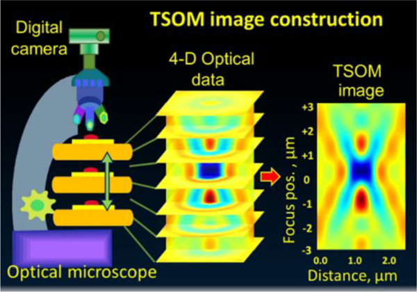
Animation depicting a typical TSOM image construction process.

A differential TSOM (D-TSOM) image is a pixel-by-pixel difference between two normalized [10, 17] and aligned TSOM images [19]. If the two TSOM images are obtained using two targets with slightly different dimensions, then the D-TSOM image color pattern highlights the type of dimensional difference between the two targets [10, 19, 22]. If the two TSOM images are obtained using the same target (similar to the repeated collection), then the D-TSOM image highlights noise [10, 17, 53], including optical and vibrational noise. Here we use the later method for noise analysis by quantifying the residual optical content in the D-TSOM image.

We use two ways to quantify the residual optical content in the D-TSOM images. The first way is by evaluating optical intensity range (OIR) metric which is defined as the absolute difference between the maximum and the minimum optical intensity in a given D-TSOM image and multiplied by 100 [19]. OIR represents the magnitude of the optical intensity difference. A second way is by evaluating the mean absolute value (MAV), calculated as:

$$MAV=\frac{1}{n}{\displaystyle \sum _{k=1}^n|}D-TSO{M|}_k$$

where n is the total number of pixels in a D-TSOM image. MAV represents total optical content in a D-TSOM image. In the current work all MAVs presented are multiplied by 1000. OIR and MAV can also be used to quantify TSOM images.

In this paper, we demonstrate that imprecise focus step size movement and the lateral displacement of sample result in increased residual signal (similar to noise) in the D-TSOM images. Hence, by quantifying the residual signal in the D-TSOM images using MAV or OIR we show that fidelity of TF image data can be evaluated. This study also shows overall noise present which affects measurement sensitivity and accuracy of the TF data.

3. Results and discussion

For the fidelity test, TF optical images of a Si line on a Si substrate with nominally 1 μm width and 100 nm height were collected using a research-grade optical microscope. Microscope conditions are as follows: illumination wavelength (λ) = 520 nm, illumination source = light emitting diode, objective magnification = 50X, objective numerical aperture (NA) = 0.55, illumination NA = 0.55, objective working distance = 9.1 mm. A bandpass filter produced illumination with a spread of approximately ± 5 nm, at the full-width-half-max level. Images were collected at 20 nm step size. The focus motor has a step size resolution of 10 nm. A black and white Peltier-cooled camera was used for image collection with a native resolution of (1388 × 1040) pixels with a bit depth of 12. However, only the central (256 × 256) pixels were used to collect the images at a high speed. Under these conditions, each camera pixel represents a distance of 65 nm. Under all the imaging conditions, illumination intensity was adjusted such that the image histogram occupies approximately the middle of the optical range. The microscope was kept on an optical table with vibration-isolation disabled so that natural vibrations are transmitted to the optical microscope, simulating stage vibrations. Color scale bar is set to automatic in all the TSOM and the D-TSOM images.

3.1. Lateral vibration analysis at a fixed focus position

First, we determined the magnitude of the stage lateral movement at a fixed focus position for different degrees of vibrations. A typical optical image of the line target set close to the best focus position is shown in Fig. 2(a). Under each of the three conditions selected 16 such repeated optical images were collected. In the first condition, a computer cooling fan (50 mm x 50 mm x 15 mm) was mounted on the optical microscope to act as a vibration source. Vibrations were transmitted to the microscope by activating (running) the fan. Images were acquired at 1 ms exposure time of the camera. In the second condition, images were collected at the same exposure time of 1 ms, but with the fan removed from the microscope reducing the vibrations. Under the third condition, a 500 ms exposure of the camera was used with the fan removed from the microscope. To achieve different camera exposure conditions, the illumination intensity of the LED light source was varied by changing its current.

Fig. 2.

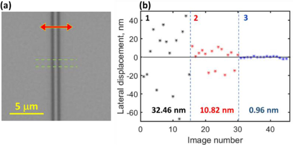
(a) A typical top-down optical image of the selected line. (b) The relative lateral displacement of the target image in the X-direction for the selected three conditions indicated at the top of the figure. Condition 1: the camera exposure time was 1 ms with simulated vibrations transmitted to the microscope from a running fan placed on the microscope. Condition 2: the camera exposure time was 1 ms without the fan. Condition 3: the camera exposure time was 500 ms without the fan. The measured standard deviations of the lateral movement under the three conditions are shown at the bottom.

Due to the presence of the vibrations, the image moves laterally proportional to the magnitude of the vibrations. This lateral movement is captured by the repeated collection of the images. Using software developed in-house, the relative distances moved in the X-direction (as shown by a red arrow mark in Fig. 2(a)) between the first image and the rest of the 15 images collected were evaluated under the three conditions with a measurement resolution of 0.01 nm. Image correlation was used for this purpose. The lateral distance was determined by minimizing the square of the difference between the two interpolated images by moving one image with respect to the other. The distance moved provides insight into the magnitude of the lateral stage movement relative to the camera and are plotted in Fig. 2(b) after adjusting with the mean center location. Comparing the results from conditions 1 and 2, we can observe that the lateral movement of the stage increases with increased vibration of the microscope as the exposure time is the same. Comparing conditions 2 and 3 where only the exposure time was changed, we can observe that increased exposure time has the effect of averaging (high-frequency) vibrations and appears to reduce the lateral stage movement. This shows that, if high-frequency vibrations cannot be reduced by other means, the effect of it can be minimized by increasing the camera exposure time which averages the images over the exposure time. The lateral vibrational analysis in the Y-direction can be evaluated similarly by orienting the line target horizontally. Alternatively, by using a suitable target such as a square, both horizontal and vertical lateral vibrations can be analyzed using the same set of images.

3.2. Effect of lateral vibrations on fidelity in through-focus image data

The TSOM images were constructed using profiles obtained by averaging 1 μm width of the image along the line at every focus position. The TSOM images presented here are minimally processed. 20 nm focus step size was linearly interpolated with one point between focus positions resulting in 10 nm focus step sizes. Spline interpolation in the lateral direction was done to obtain a lateral resolution of about 10 nm.

As observed in the previous section, the magnitude of the effective image lateral movement due to the stage vibration can be reduced by increasing the camera exposure time. Hence, to study the effect of the stage mechanical lateral vibrations on the fidelity, TF images were collected at the camera exposure times of 500 ms. The TSOM images were extracted at two focus step sizes of 100 nm and 250 nm. The selection of the two step sizes (100 nm and 250 nm) was to evaluate and demonstrate any dependence of step size on the fidelity test results. This is the typical range of step sizes most commonly selected for the TSOM analysis. A typical TSOM image of the line target is shown in Fig. 3(a). For clarity, the relative orientation of the TSOM image and the optical image is shown in Fig. 3(b).

Fig. 3.

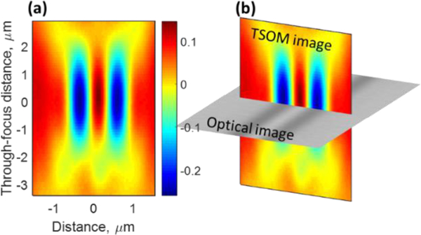
(a) TSOM image of the selected line target at 100 nm step size. (b) Figure depicting relative orientations of the optical and the TSOM images.

D-TSOM images obtained using two repeated measurements of TSOM images of the same line target under the same conditions will include noise due to mechanical lateral and vertical vibrations, in addition to other sources of noises, e.g., optical noise. The effect of mechanical vibrations can be nearly eliminated by taking D-TSOM images from two TSOM images constructed from the same set of TF images. For example, a D-TSOM image extracted from the two TSOM images obtained from the two locations as marked by the dashed lines in Fig. 2(a) would produce a D-TSOM image with noise originating mostly from non-mechanical sources (Fig. 4(a)). The lateral and vertical mechanical vibrations would be nearly equal at these two locations on the same image from the same TF data and hence would cancel out in the D-TSOM images. This provides the base-noise originating from non-mechanical vibrations.

Fig. 4.

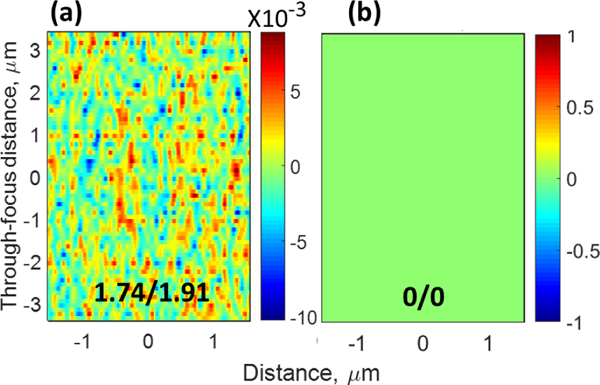
D-TSOM images representing (a) typical non-mechanical sources of noise, and (b) zero noise. Numbers in the inset are MAV/OIR values.

In the current setup used, MAV and OIR of the average base-noise are 1.74 and 1.91, respectively (from 20 repeats). Standard deviations of the MAV and OIR are 0.02 and 0.09, respectively. MAV with relatively less standard deviation seems to produce a more stable representation of the noise value compared to OIR. Even though it is obvious, for a comparison we present a D-TSOM image from the same location, using the same TF data, in Fig. 4(b) that shows a zero-noise level.

Having known the noise level originating from typical non-mechanical sources, we then first explore the effect of lateral vibrations/movement of the image due to mechanical instability on the resultant noise magnitudes of the D-TSOM images. Mechanical vibrations could be one of the sources of the lateral image movement. For this, we collected TF images with an exposure time of 500 ms. After constructing a relatively stable TSOM image (similar to Fig. 3(a)), image profiles at every focus position were then moved with a magnitude that is random in the lateral direction (i.e., perpendicular to the line or in the X-direction as shown in Fig. 2(a) by an arrow mark) with magnitudes of ±20 nm, ±40 nm, and ±80 nm, from the mean original positions with Gaussian distribution. The resultant typical TSOM images are shown in Figs. 5(a) to 5(c) for 100 nm step size. The smallest lateral movement possible was chosen to be 10 nm. Hence, for the 0 nm to ±20 nm condition, the lateral movements possible were −20 nm, −10 nm, 0 nm, +10 nm and +20 nm. Similarly, under the other conditions used here, the number of possible movements increases with the magnitude of the maximum lateral movement. Using the same measured TSOM image, several such TSOM images were generated with random lateral movements of profiles at each focus position for each TSOM image. Typical D-TSOM images for the different maximum magnitude lateral movements are shown in Figs. 5(a1) to 5(c1). A similar process was repeated for 250 nm step size TSOM and D-TSOM images as shown in Figs. 5(d) to 5(f) and Figs. 5(d1) to 5(f1), respectively.

Fig.5.

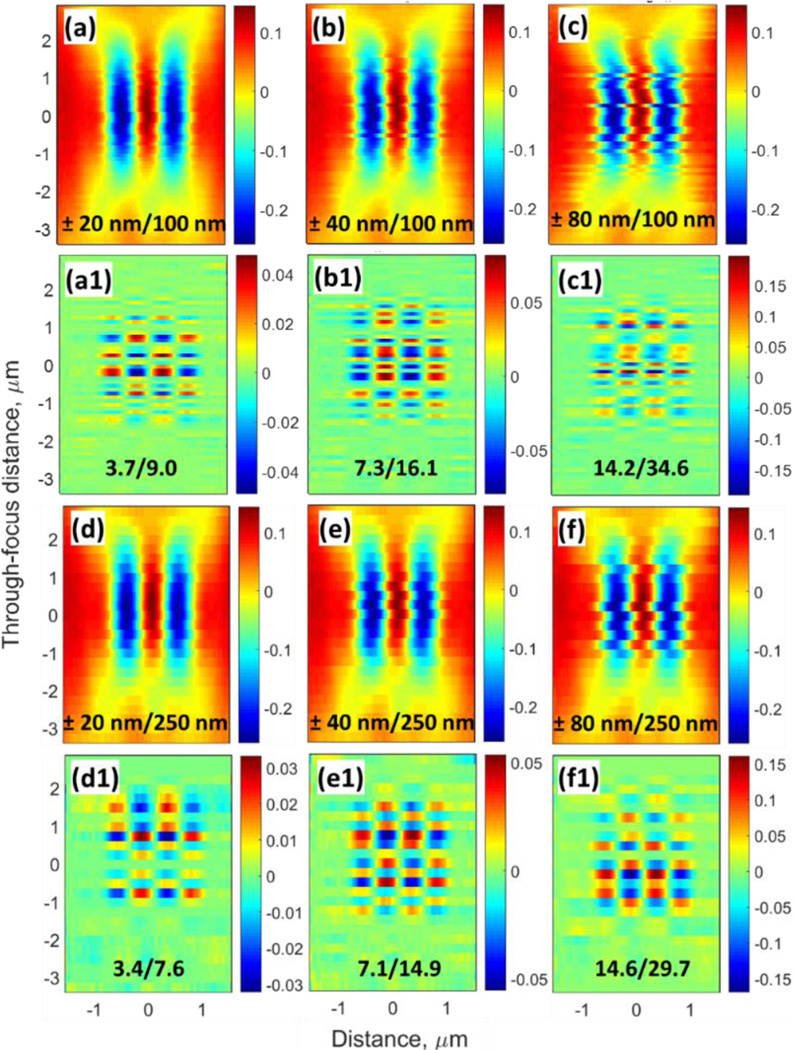
Effect of the simulated random mechanical lateral stage vibrations of different magnitudes during TF image collection. (a), (b), and (c) Typical TSOM images with 100 nm step size for lateral stage vibrations of 0 nm to ±20 nm, ±40 nm, and ±80 nm, respectively. (a1), (b1), and (c1) Typical D-TSOM images between two TSOM images generated similar to (a), (b), and (c), respectively. (d), (e), and (f) Typical TSOM images with 250 nm step size for lateral stage vibrations of 0 to ±20 nm, ±40 nm, and ±80 nm, respectively. (d1), (e1), and (f1) Typical D-TSOM images between two TSOM images generated similar to (d), (e), and (f), respectively. Numbers in the inset of (a) to (f) indicate lateral maximum vibrations and focus step size. Numbers in the inset of (a1) to (f1) indicate mean MAV/OIR values from 20 repeats.

Increased noise can be expected with increased magnitude of the lateral movement. This noise was quantified using MAV and OIR. The average and standard deviations of MAVs and OIRs from 20 such D-TSOM images generated were extracted for the selected maximum magnitude lateral movements for the 100 nm and 250 nm step sizes. This provides the effect of purely lateral image movement on the resultant noise. This also indicates the effect of the lateral vibrations on the fidelity of the TSOM images. To include noises originating from nonmechanical sources (Fig. 4(a)), we repeated the same process using two separate TSOM images extracted from several repeats. Both sets of results are plotted in Figs. 6.

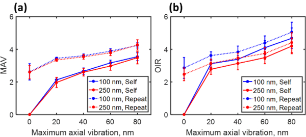
Fig. 6.

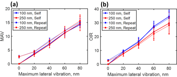
Mean D-TSOM image noise levels as extracted by (a) MAV, and (b) OIR, for different simulated maximum lateral vibrations at two focus steps sizes of 100 nm and 250 nm. ‘Self’ indicates D-TSOM image obtained using random lateral vibrations applied on the same TSOM image. ‘Repeat’ indicates D-TSOM image obtained using random lateral vibrations applied on repeated collections of the TSOM images from the same line target. Error bars represent one standard deviation using 20 data points.

As expected, it can be observed from Fig. 6 that under all the conditions, increasing lateral vibrations increased the noise level, whether non-mechanical noises are included or not. Addition of the non-mechanical noises increased the overall noise level measured using MAV metric, which is also expected, but by not a significant level. Not much difference in the noise levels can be observed between 100 nm and 250 nm step sizes if the noise is quantified using MAV. However, if the noise is quantified using OIR, 250 nm step size mostly produces a lower noise level compared to the 100 nm step size (Fig. 6(b)). Depending on the type of metric used to quantify noise, under certain conditions slightly different trends can be observed. However, MAV which represents a mean noise level appears to be a better way to quantify the noise as opposed to the peak-to-valley difference in the optical noise as represented by OIR because of the following reasons:

1. Addition of the non-mechanical sources of noise in principle should increase the overall noise. This increase is visible only if the noise is quantified using MAV (Fig. 6(a)).

2. Whether using 250 nm or 100 nm step sizes the noise level should scale with the maximum lateral vibrations. MAV appears to track this well (Fig. 6(a)).

3. In addition, OIR appears to have a larger standard deviation as a percentage of the mean value when compared to MVA (Fig. 7 (a)), indicating MVA could be a more stable noise level metric compared to OIR.

Fig. 7.

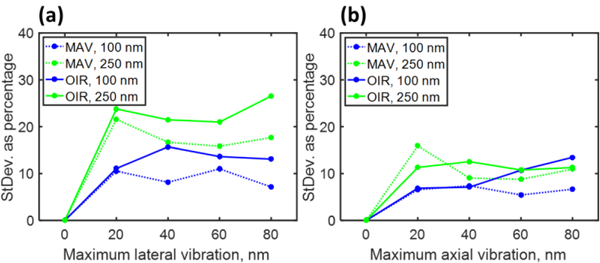
One standard deviation of the noise extracted using MAV and OIR metrics as a percentage of the mean values obtained from repeating the process 20 times for (a) lateral, and (b) axial vibrations. The D-TSOM images were extracted using random vibrations applied to the same (‘self’) TSOM image.

3.3. Effect of axial vibrations on fidelity of through-focus image data

The effect of vibrations and imprecise focus step sizes in the focus (axial) direction was studied in a similar way. TF images were initially collected using a step size of 20 nm and an exposure time of 500 ms; the resulting data were then interpolated to make a 10 nm step size. TSOM images with either 100 nm or 250 nm step sizes were then extracted by skipping either 9 or 24 TF images, respectively, from this set of TF images. The step size is constant in the absence of axial vibration. This produces TSOM images with nominally no vibration along the focus direction. The presence of axial vibrations either increases or decreases the step size. For this reason, while extracting the TSOM images, the effect of the axial random vibrations was artificially accomplished either by increasing or decreasing the nominal step sizes. The presence of ±20 nm maximum axial vibration from the nominal step size results in possible instantaneous focus step sizes of 80 nm, 90 nm, 100 nm, 110 nm and 120 nm for a 100 nm step size TSOM image. For each step, one of these possible step sizes were randomly selected resulting in a TSOM image with a random maximum axial vibration of ±20 nm. In the current demonstration study, since the smallest step size is 10 nm, the smallest axial vibration that can be achieved in the way described is limited to 10 nm. However, the actual instantaneous random axial vibration can vary from zero to the maximum possible level.

Typical TSOM and D-TSOM images extracted in the manner explained above for 100 nm and 250 nm step sizes and ±20 nm, ±40 nm, and ±80 nm, maximum axial vibrations are presented in Fig. 8. Comparing Figs. 5 and 8, it can be observed that the axial vibrations have significantly less discernible deviation from the nominally zero vibration TSOM images for both 100 nm and 250 nm step sizes (Figs. 8(a) to 8(f)). The resultant mean axial noise is also significantly less compared to the mean lateral noise. In addition, the noise is more uniformly distributed across the D-TSOM images (Figs. 8(a1) to 8 (f1)). While lateral noise is most heavily concentrated around the higher optical intensity locations in the TSOM images (Fig. 5), where the intensity gradient is large.

Fig.8.

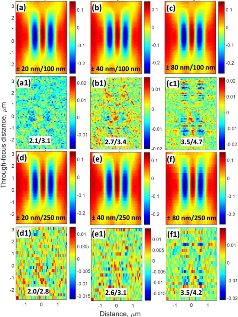
Effect of the simulated random mechanical stage vibrations in the focus (axial) direction of different magnitudes during TF image collection. (a), (b), and (c) Typical TSOM images with 100 nm step size for axial stage vibrations of 0 nm to ±20 nm ±40 nm, and ±80 nm, respectively. (a1), (b1), and (c1) Typical D-TSOM images between two TSOM images generated similar to (a), (b), and (c), respectively. (d), (e), and (f) Typical TSOM images with 250 nm step size for axial stage vibrations of 0 to ±20 nm, ±40 nm, and ±80 nm, respectively. (d1), (e1), and (f1) Typical D-TSOM images between two TSOM images generated similar to (d), (e), and (f), respectively. Numbers in the inset of (a) to (f) indicate axial maximum vibrations and focus step size. Numbers in the inset of (a1) to (f1) indicate mean MAV/OIR values from 20 repeats.

Mean noise as quantified using MAV and OIR resulting from increased axial maximum vibrations are presented in Fig. 9 for both 100 nm and 250 nm focus steps. Similar to the lateral vibrations, the axial vibrations also increase the noise with increased maximum axial vibrations. Addition of the non-mechanical noises increases the overall noise level. Not much difference in the noise levels can be observed between 100 nm and 250 nm step sizes for the noise quantified using MAV. However, a few significant differences can be identified, whether nonmechanical noises are included or not. The rate of increase in noise with increased maximum axial vibration is significantly smaller compared to the lateral vibrations (Fig. 6). Overall noise is also significantly less compared to the lateral vibrations. In terms of percentage increase, the addition of non-mechanical noises increases the overall noise level substantially over the noise without addition of non-mechanical noises. In this case, the standard deviation of the noise as a percentage of the mean noise levels is mostly similar for the noise quantified using either MAV or OIR (Fig. 7(b)).

Fig. 9.

Mean D-TSOM image noise levels as extracted by (a) MAV, and (b) OIR, for the different simulated maximum axial vibrations at two focus steps sizes of 100 nm and 250 nm. ‘Self’ indicates D-TSOM image obtained using random axial vibrations applied on the same TSOM image twice. ‘Repeat’ indicates D-TSOM image obtained using random axial vibrations applied on repeated collections of TSOM images from the same line target. Error bars represent one standard deviation using 20 data points.

3.4. Effect of the combined lateral and axial lateral vibrations on fidelity of through-focus image data

The effect of combining the lateral and the axial vibrations on the noise level was also studied. For this study, the same maximum vibration values were selected for both the lateral and the axial vibrations. The results are presented in Fig. 10. Since the noise resulting from the lateral vibrations (Fig. 6) is significantly higher than the axial vibrations (Fig. 9), the combined noise level appears to be dominated by the trend observed by the lateral vibration only. This suggests that it is important to aggressively minimize the lateral vibrations compared to the axial vibrations to reduce the overall noise levels.

Fig. 10.

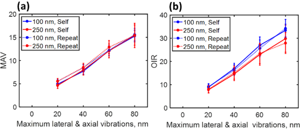
Mean D-TSOM image noise levels as extracted by (a) MAV, and (b) OIR, for the different simulated maximum lateral and axial vibrations together at two focus steps sizes of 100 nm and 250 nm. ‘Self’ indicates D-TSOM image obtained using random lateral and axial vibrations applied on the same TSOM image twice. ‘Repeat’ indicates D-TSOM image obtained using random lateral and axial vibrations applied on repeated collections of TSOM images from the same line target. Error bars represent one standard deviation using 20 data points.

So far, we have presented the effect of artificially created random lateral and axial vibrations on the noise levels. Here, we study the effect of naturally occurring vibrations (combined lateral and vertical) and their effect on the final vibration levels. For this, TF data were collected using camera exposure times of 1 ms, 10 ms, 100 ms and 500 ms at a focus step size of 200 nm (but linearly interpolated to get a focus step of 100 nm) while transmitting naturally occurring vibrations to the microscope by deactivating vibration-isolation of the optical table on which the optical microscope is placed. Only at 1 ms exposure time, vibrations were increased using a running fan as before. At least seven repeated TF images were taken at each of the conditions. As seen above (Fig. 2), increasing camera exposure time is expected to reduce the effect of the vibrations by averaging them during the exposure time. Extracted typical TSOM and D-TSOM images are presented in Fig. 11. As expected increased camera exposure time reduced the effect of the vibrations and hence the noise levels in the TSOM (Figs. 11 (a) to (d)) and D-TSOM images (Figs. 11 (a1) to (d1)). Based on this it can also be observed that increasing the camera exposure time could be one way to reduce the overall noise. The mean noise as measured using MAV/OIR are indicated in Figs. 11 (a1) to (d1). The mean MAV/OIR values along with their standard deviations presented in Fig. 12 from 20 measurements shows a decreasing trend of the noise with increasing the exposure time.

Fig. 11.

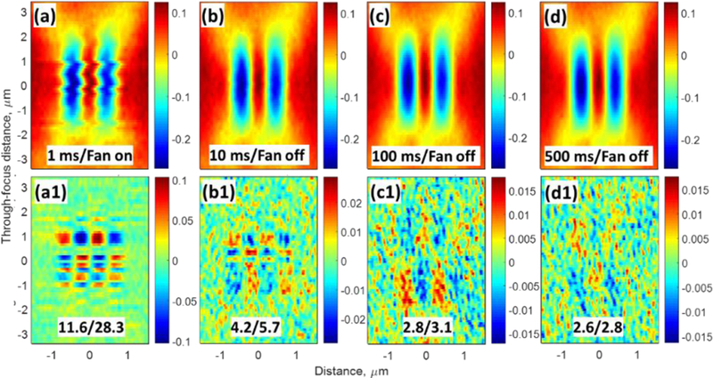
Effect of the increased camera exposure time on the natural mechanical stage vibrations detected during TF image collection. (a), (b), (c) and (d) Typical TSOM images with 100 nm step size for different camera exposure. (a1), (b1), (c1) and (d1) Typical D-TSOM images between two TSOM images generated similar to (a), (b), (c) and (d), respectively. Numbers in the inset of (a) to (d) indicate camera exposure time and activation condition of the computer cooling fan placed on the microscope. Numbers in the inset of (a1) to (d1) indicate mean MAV/OIR values from 20 repeats.

Fig. 12.

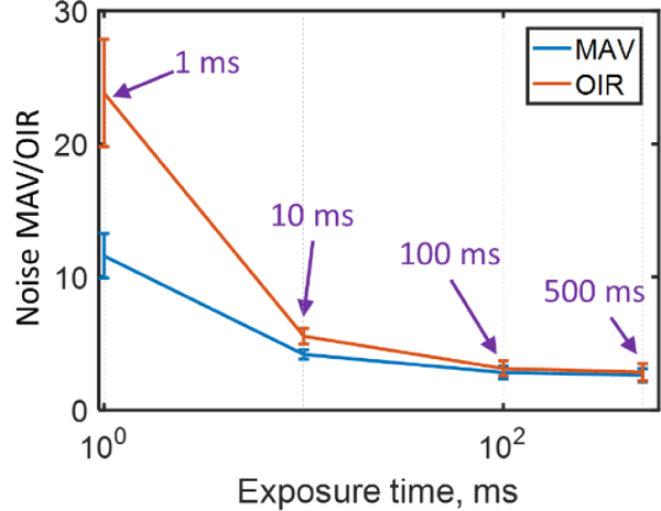
Mean noise as measured by MAV/OIR with increased camera exposure time. The error bars represent one standard deviation using 20 measurements.

3.5. Effect of other issues on fidelity of through-focus image data

So far, we have assumed that as the stage traverses along the focus direction its lateral movements are random from the mean central distance. This occurs when the focus axis of the stage coincides with the optical axis of the optical microscopes. However, for some microscopes, the focus axis of the stage may not coincide with the optical axis of the microscopes. Under these circumstances, it appears as if the stage (and hence the optical image) moves laterally in one direction as the stage scans along the focus direction. This condition results in a TSOM image as shown in Fig. 13 (a), where its axis (indicated using a dashed line) is inclined. It is strongly advised to rectify the inclination of the TSOM axis for accuracy. However, even if the stage axis aligns with the microscope optical axis, the similar tilt in the TSOM axis (Fig. 13(b)) could arise due to illumination aberrations arising from misalignment of the aperture diaphragm in microscopes [15, 52, 54]. Hence to rectify it, care must be taken to identify the correct source of the TSOM axis inclination.

Fig. 13.

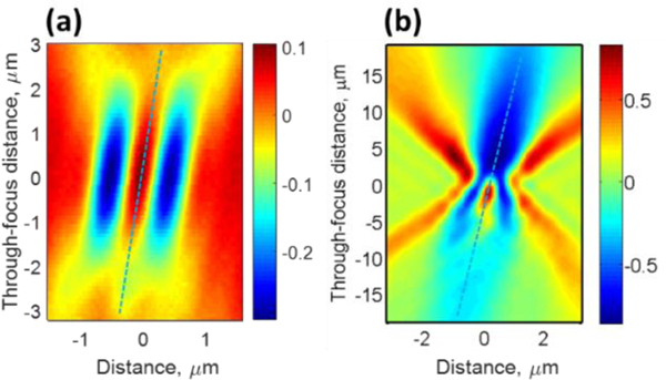
Tilt in the TSOM axis shown by dashed lines due to (a) the stage unidirectional lateral movement (in this case 10 nm lateral shift to the right for each focus step), and (b) misalignment of the aperture diaphragm (reproduced from [15]).

4. Summary

In a first attempt to standardize TF image collection protocols, here we presented a method to determine the fidelity of the TF optical images using TSOM. Lateral and axial vibrations/movements during mechanical focus scanning are the two aspects uniquely associated with the TF type of imaging. Mechanical instability and ineffective noise isolation of the optical tool could be two of the many possible reasons for the vibrations. We studied the effect of random lateral and axial vibrations on the resulting noise as evaluated by D-TSOM images. The noise was quantified using MAV and OIR. Under most of the conditions, both MAV and OIR provided similar types of trends and conclusions. However, under all the conditions MAV seems to be a better metric for noise. An important conclusion is that the lateral vibrations result in a significantly larger noise level compared to the axial vibrations for the similar magnitude of vibrations. To minimize vibrations and hence to increase the fidelity of the TF optical data, a larger emphasis must be given to reduce the lateral vibrations during the TF image collection process. One way to decrease the effect of lateral vibrations is to increase the camera exposure time, if possible. Another way to enhance the fidelity of the TF data is to minimize (or eliminate) the causes that result in inclination in the axis of TSOM images.