Assimilating Radial Distribution Functions to Build Water Models with Improved Structural Properties

Abstract

The structural properties of three and four site water models are improved by extending the ForceBalance parameterization code to include a new methodology allowing for the targeting of any radial distribution function (RDF) during the parametrization of a force field. The mean squared difference (MSD) between the experimental and simulated RDFs contributes to an objective function, allowing for the systematic optimization of force field parameters to reach closer overall agreement with experiment. RDF fitting is applied to develop modified versions of the TIP3P and TIP4P/2005 water models in which the Lennard-Jones potential is replaced by a Buckingham potential. The optimized TIP3P-Buckingham and TIP4P-Buckingham potentials feature 93 and 98 percent lower MSDs in the OO RDF compared to the TIP3P and TIP4P/2005 models respectively, with marked decreases in the height of the first peak. Additionally, these Buckingham models predict the entropy of water more accurately, reducing the error in the entropy of TIP3P from 11 to 3 percent and the error in the entropy of TIP4P/2005 from 11 to 2 percent. These new Buckingham models have improved predictive power for many non-fitted properties particularly in the case of TIP3P. Our work directly demonstrates how the Buckingham potential can improve the description of water’s structural properties beyond the Lennard-Jones potential. Moreover, adding a Buckingham potential is a favorable alternative to adding interaction sites in terms of computational speed on modern GPU hardware.

Introduction

The water molecule has been studied in great detail with significant attention from experimental and theoretical works [1] [2] [3] due to its ubiquity and many unique properties such as a large heat capacity and its expansion when frozen. With such a large amount of attention given to water, naturally there are a wide range of atomistic water models for molecular simulation [4] [5] [6] [7]. The variation in these models comes from the different approximations made in the model or which properties of the system have been targeted during their parametrization. Within the space of rigid water molecules, TIP3P [4] and TIP4P/2005 [8] are common three and four site water models used in biomolecular simulation and are the starting point of our study. Improving the accuracy of modelling water enables studies of biochemical mechanisms with atomic resolution, for example protein-ligand binding [9] or protein folding [10]. Some of the crucial properties for the accuracy of these simulations are the entropy and enthalpy. The entropy is strongly linked with the structural properties and correlation in a fluid and it is therefore important to note that water exhibits significantly more correlation than a simple LJ fluid of comparable densities [11].

This work focuses on classical water models designed for classical molecular dynamics (MD) simulation. Compared to more exact quantum mechanical methods, classical MD and the associated potentials employ many approximations intended to describe much of the physics underlying the behavior of a system implicitly. For example, water models with nonpolarizable effective pair potentials do not allow for the redistribution of charge on a molecule’s atoms, resulting in the neglect of any induced dipoles. The permanent dipole of the model may be fitted to include the averaged induced dipole for a chosen density, but the approximation will start to fail as the density and intermolecular separations start to deviate from the parameterization conditions. Additional approximations pertain to the intramolecular vibrations, and their temperature dependence, which are neglected by rigid water approximations. Ideally these vibrational effects would receive a quantum mechanical treatment, however in the absence of this, many water models [8] [12] will apply corrections to reproduce raw experimental data.

Considering these approximations, the difficulty in selecting potential forms and parameters that can reproduce a wide range of properties over a wide range of temperatures and pressures becomes clear. Historically, the parametrization of force fields has been described as a “black art” [13] because modifying parameters, running simulations, calculating properties, and comparing with experiments involves a complicated workflow that is arduous to perform manually and can be difficult to reproduce. The ForceBalance code [14] addresses the challenge of reproducibility by enabling diverse types of parameterization calculations in a common software framework. In this work, our goal is to improve the agreement of water’s simulated structural properties with experiment for two common water models using ForceBalance as a principal tool.

Radial distribution functions

A radial distribution function (RDF) describes the structure of a molecular system as the variation in particle number density with distance from a reference particle. Equation (1) [15] shows how a RDF could be calculated.

$$g_{\alpha \beta }(r)=\underset{dr\to 0}{\text{lim}}\frac{\rho (r,dr)}{4\pi (N_{\alpha \beta }/V)r^{2}dr}$$ (1)

Here r is the distance between the atom pairs, ρ(r, dr) is the number of atom pairs in the infinitesimal shell spanning r to r + dr (averaged over all trajectory frames), N_αβ is the number of pairs for the two species considered and V is the volume of the system. ρ(r, dr) is normalized to the uniform density of an ideal gas; thus any deviation for the value of g_αβ(r) from unity is the result of some order or correlation in the material. While an RDF can’t be used as a unique fingerprint for a material it can be a robust description. RDFs can be informative of bond lengths and coordination number, and can be used to calculate many thermodynamic properties assuming the potentials describing the system are pairwise additive [16]. Moreover, RDFs can be derived from experimental X-ray or neutron diffraction data to provide robust comparisons between simulation and experiment.

Water can cause potential complications in the calculation of the experimental RDFs due to the presence of light and weakly charged hydrogen. X-ray diffraction is a good tool to calculate the OO RDF, but less information about HH and OH RDFs can be extracted [17]. Neutron diffraction methods also have difficulty with hydrogen, as the low atomic weight makes it difficult to approximate the neutron scattering as elastic, and this inelasticity complicates the measurement. As a treatment the inelasticity can be modelled [1] or isotope substitution can be used. In 1982 Soper [1] used the latter to make a calculation of water RDFs. The neutron diffraction Soper data from 2000 [17] was used as the experimental reference in this work. The RDFs in Soper’s work are calculated at 298K and 1atm of pressure.

Entropy

One benefit of accurately reproducing the experimental RDF is improving calculations of the excess entropy. The link between the excess entropy and RDF are clear when considering the RDF as a measure of correlation in atoms. RDFs as presented can be used to calculate the translational two-body entropy of a fluid and these calculations can be seen more formally in the work of Hernando [18] and Laird et al [19].

For a molecular fluid such as water, an additional orientational component to the two-body entropy exists. Studies which look at the entropy of water beyond the two-body translational term have been carried out by Lazaridis et al [11] and conclude that within the two-body entropy there is a significant contribution from the orientational correlation, around three times the translational excess entropy when studying TIP4P. Considering this, to improve the computed excess entropy for water, it would be beneficial to target the orientational correlation of a fluid via an orientational distribution function (ODF). However, in the case of water this is much more expensive to compute the than the RDF with the relative orientation defined by five angles. Even if computed the ODFs cannot be compared to experimental data by calculating a MSD, as there is currently no method to extract the ODF directly from experiment [20] [21]. Consequently, ODFs are not compatible with the presented fitting methodology, which relies on a MSD, and as such will not be targeted in this work. However, the RDF still can and will be used as a target property.

Water Models

For later reference and for clarity, a presentation of the 3D models of TIP3P and TIP4P are presented in Figure (1). Both models are rigid and nonpolarizable, and have a single VDW site located on the position of the oxygen and partial charges on the hydrogen positions. TIP3P has a negative partial charge on the oxygen atom whereas TIP4P places this charge on a fourth (virtual) site. [22] The fourth site was originally explored by Bernal and Fowler [2] with the site introduced to allow for the screening if the hydrogen charge, moving some of the charge distribution towards the hydrogens along the HOH bisector; it also allows for the charge distribution to be varied independently of the HOH geometry or dipole.

Figure 1.

Representation of TIP3P and TIP4P geometries. TIP3P left and TIP4P right. Oxygen shown in red, hydrogen in white and the TIP4P virtual site in blue. HOH are bonded with angle between them θº. The virtual site position is defined as a function of atomic positions, and placed along the HOH angle bisector. l₁[Å] is the OH bond length and l₂[Å] is the distance between oxygen and the virtual site.

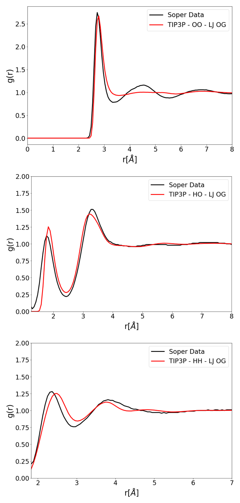
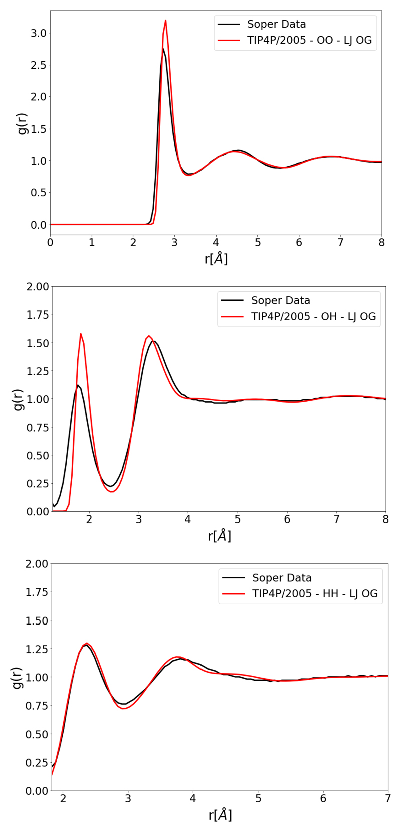
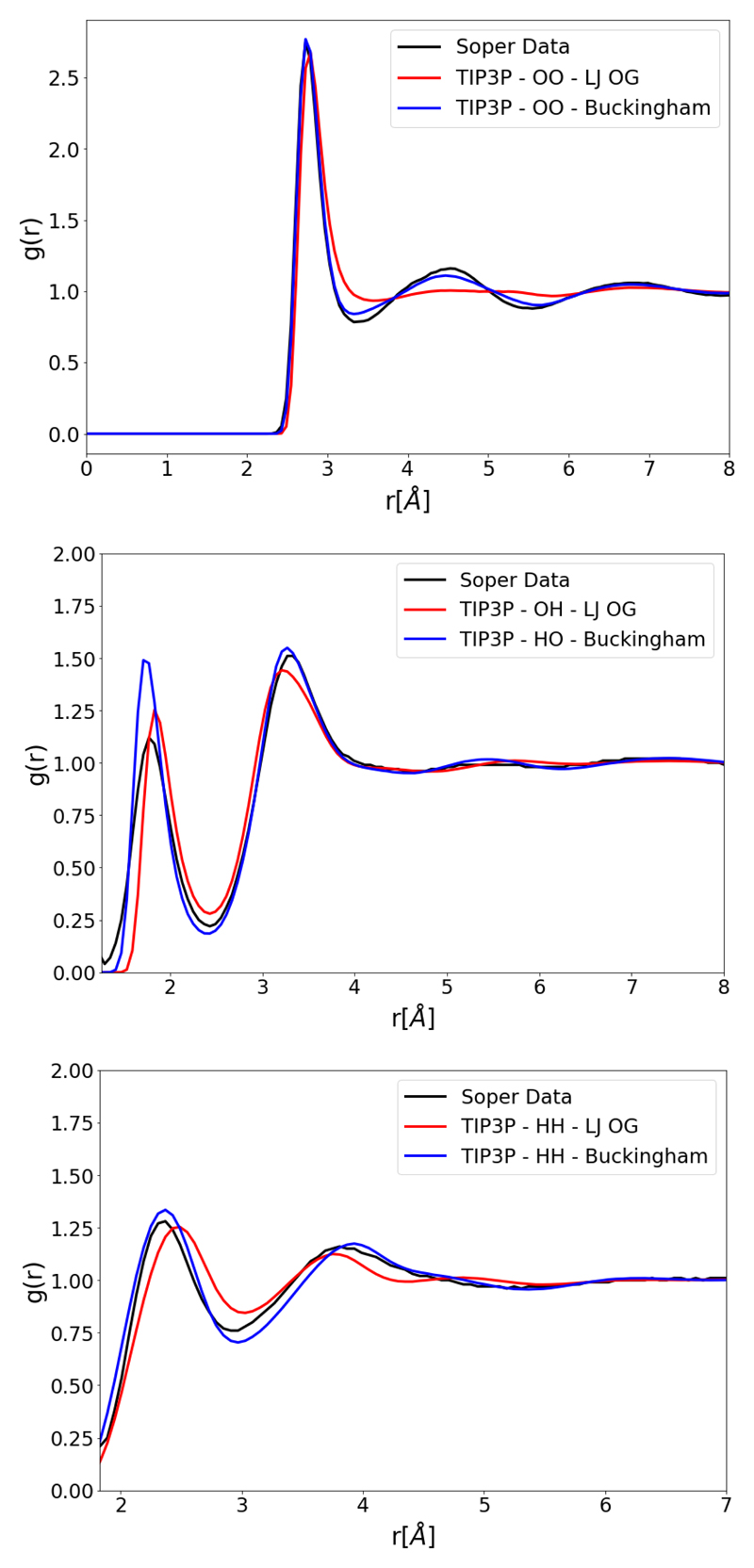
TIP3P is a reparameterization [4] of an earlier three-point model TIPS built by Jorgensen et al [3]. TIPS force fields were built as part of an effort to simulate many solvents including water, alcohols, and ethers. TIP3P is one of the more common models with large under-structuring in the second and third shells, as seen in Figure (2); this is somewhat corrected by more recent work to parametrize this force field for use with Ewald summations [5]. TIP4P-type models again have several parametrizations such as TIP4P [6], TIP4P/2005 [8] and TIP4P/ICE [23]. TIP4P was reparametrized as TIP4P/2005 by Abascal et al [8] with a fit based on the temperature of maximum density. TIP4P/2005 shows good agreement for many properties particularly the density; however the simulated RDFs differ from experiment, with the first peak on the OO RDF showing marked over-structuring as shown in Figure (3). Other parametrizations using ForceBalance with three and four site models have been performed previously [14], focusing on improving agreement for thermodynamic properties. The resulting TIP3P-FB and TIP4P-FB models provided improved predictive power for the kinetic properties such as the self-diffusion coefficient, but these models still have over-structuring in their RDFs similar to TIP4P/2005.

Figure 2.

OO, OH and HH RDFs for the original TIP3P parametrization (TIP3P-LJ OG) compared to Soper data. [17]

Figure 3.

OO, OH and HH RDFs for the original TIP4P/2005 parametrization (TIP4P-LJ OG) compared to Soper data. [17]

The LJ interaction in these TIPnP models is of particular interest. Soper highlighted the possibility that the r⁻¹² term is too repulsive and may be the cause of much of the over-structuring seen in the first shell of the OO RDF; [24] an additional exponential term was added to the non-bonded potential with the aim of softening the LJ interaction. The discussion by Wheatley et al on the approximately exponential nature of inter molecular repulsion [25] makes the Buckingham potential [26] a good candidate to replace the LJ. Wang et al [27] applied a modified version of the Buckingham potential in the parametrization of a polarizable water model, where the functional form was altered to remove the singularity at the origin. Despite these efforts, the first shell of the OO RDFs of these models remained over-structured compared to experiment, with one possible cause attributed to the lack of nuclear quantum effects in the classical simulations [27].

Materials and Methods

Radial distribution function fitting

ForceBalance is a program which allows for the systematic fitting of force field parameters [13] by including bulk properties taken from experiment and/or high-level theoretical calculations in the objective function. In this work, ForceBalance is extended to target any RDF of any material. During the fitting procedure, ForceBalance carries out a MD simulation by calling external simulation software; the MD simulations in this work are performed by OpenMM; [28] this code includes GPU-accelerated implementations of the force fields and simulation methods. Simulation snapshots are saved at equally spaced time intervals, and a calculation of each targeted property is made for each snapshot. The RDF calculation from snapshot coordinates is handled by MDTraj [29], a Python library that focuses on fast MD trajectory analysis. Once the RDFs for all snapshots are computed, a mean squared difference (MSD) is calculated between them and an experimental RDF, provided by the user. The MSD is calculated for every snapshot individually before any averaging. This MSD when weighted contributes to the objective function in the fitting procedure, with Equation (2) showing the calculation the MSD.

$$A=\frac{{\sum }_n{(RD{F}_n^{comp}-RD{F}_n^{\mathit{\text{exp}}})}^2}{N}$$ (2)

A is the MSD for a one of the targeted RDFs in one snapshot, averaging across snapshots will give an ensemble average of the MSD 〈A〉. n indexes the bins in the histogram of the RDF. RDF^comp is the computed and RDF^exp the experimental RDFs. N is the total number of bins, which is set by the number of data points in the experimental RDF provided by the user. To change the relative contribution of RDFs to the objective function the MSD can be multiplied by a user defined pre-factor that sets the relative weights for the different RDF targets; the weights in this work are provided in Table (1). The optimization carried out in this work took place in two steps: first allowing all the models parameters, excluding the geometric parameters to be optimized and then following this with further optimization of all parameters including geometric parameters. This was done to keep bond angles and lengths close to physical values and mitigate problems of over fitting. When running an optimization, the pre-factor for each residual in the objective function is specified. These pre-factors are chosen differently between the two runs of optimization and are shown in Table (1). The pre-factors in the optimization are chosen initially (Initial) in-line with Wang et al’s [14] work on ForceBalance. The revised (Revised) pre-factors in the continuation of the optimization are chosen to approximately normalize the contribution of the properties residual to the objective function during optimization and reflect the desire to achieve better experimental agreement for H_vap, with the aim of ultimately improving agreement with experimental free energies.

Table 1.

Relative Pre-factors of Target Properties Used in the Two^a Runs of Sequential Parameter Optimization. Pre-factors Presented are for Density ρ, Enthalpy of Vaporization H_vap and MSDs Between Experimental and Computed RDFs OO-MSD, OH-MSD and HH-MSD.

	ρ	Hvap	OO − MSD	OH − MSD	HH − MSD
Initial	1	0.16	1000	1000	1000
Revised	1	1600	40000	20000	100000

^aFirst run is denoted Initial second as Revised. Pre-factors are presented as relative to the pre-factors of the density.

To minimize the objective function efficiently, ForceBalance needs the gradient of the target property w.r.t the fitting parameters, Equation (3) shows how this gradient is calculated.

$$\frac{d\langle A\rangle }{d\lambda }=-\beta \left(\langle A\frac{dE}{d\lambda }\rangle -\langle A\rangle \langle \frac{dE}{d\lambda }\rangle \right)$$ (3)

Above λ is the parameter which is being optimized, β the reciprocal of the temperature and Boltzmann constant product. E is the potential energy. dE/dλ is evaluated in ForceBalance by the post processing of the collected trajectories. More detail on this and the general ForceBalance methodology can be found in the ForceBalance papers [14] [13].

A feature of ForceBalance is the specification of rescaling factors (also called prior widths) for the optimization parameters; these have the dual effect of improving the Hessian condition number used in the optimization algorithm, and secondly to limit how much the physical parameters can vary during optimization. In this work, the priors are set to the ForceBalance default value, which means the prior for each observable takes the value of that observable. In all the presented work, the nearest-neighbor OH and HH peaks corresponding to intramolecular distances are omitted as the models being optimized are rigid; improving the agreement in these peaks would require a flexible model and/or treatment of nuclear quantum effects.

Parametrization simulations

Two sets of optimization calculations were made in this work. The first set involves fitting of TIPnP models using the LJ potential, and the second set involves fitting alternative versions of the TIPnP models where the LJ potential is substituted by a Buckingham potential. All non-bonded and geometric parameters were fit unless specified otherwise. Each step of optimization involved running a simulation with a total length of 6 ns; the simulation time step used was 2 fs. Simulation snapshots are saved and bulk properties / RDFs calculated at 20 ps intervals, providing 300 data points over the trajectory. The experimental RDF was taken from neutron diffraction experiments [17]; the other data used for fitting was the enthalpy of vaporization ΔH_vap = 43.989 kJmol⁻¹ and density ρ = 997.045 kgm⁻³ for a temperature of 298°C and 1 atm of pressure [14]. These simulations were performed in the NPT ensemble using the Langevin integrator with 1 ps⁻¹ time constant and a Monte Carlo Barostat with volume changing moves every 50 fs. A switching distance of 9 Å and cutoff of 11 Å was used with PME treating the long range electrostatic interactions; the Ewald tolerance was set to 5×10⁻⁴. The optimizations used 25-30 Å water cubes containing 512-895 molecules with periodic boundary conditions. Self-polarization corrections were applied for the calculation of the heat of vaporization with the permanent dipole moment µ_o = 1.855 Debye and polarizability α = 1.47 ų [30]. The RDFs for final presentation in the results section were calculated after the fitting under the same conditions, however, now using a 10 ns trajectory and 1 ps snapshot allowing for better converged values.

Buckingham potential

The Buckingham potential can be used by OpenMM within the custom force feature. Using the functional form shown in Equation (4) [27]. There are now three parameters that needed to be fit ε, R_min and γ.

$$V_{b0}=\frac{\epsilon }{1-6/\gamma }\left[\frac{6}{\gamma }{e}^{\gamma (1-\frac{r}{R_{min}})}-{\left(\frac{R_{min}}{r}\right)}^6\right]$$ (4)

Here ε is the well depth, R_min is the position of minimum energy and γ a constant which controls the repulsiveness. The singularity at a radial distance of zero should be noted; for small enough γ values, particles can jump over the repulsive barrier falling into the singularity producing unphysical results. In the calculations presented here, γ never enters a region of parameter space which would allow for this jumping to become a problem. This Buckingham potential is added to the oxygen in place of the LJ potential.

Free energy calculations

To assess the claim that fitting to the RDF will improve the entropy of bulk water these entropies must be calculated. The calculation of the entropy will be made from calculations of the Gibbs free energy and enthalpy following the definition of the excess free energy given in Equation (5).

$$G_{excess}=H_{excess}-T{S}_{excess}$$ (5)

Where G_excess is the excess free energy, H_excess the excess free enthalpy which is equivalent to - H_vap and TS_excess temperature multiplied by the excess entropy. If the free energy and enthalpy are calculated the entropy can be accessed. The enthalpy was calculated within ForceBalance via a fluctuation formula and this was done during the fitting, with the computed values presented in Table (2). The free energy calculations require additional work to compute. For this YANK [31] a GPU accelerated platform for alchemical free energy calculations was used.

Table 2.

Calculated Properties for Original and Re-parametrized Water Models. Experimental Data Taken from [14], [20] and [32]: Density ρ, Enthalpy of Vaporization H_vap, Static Dielectric Constant ϵ(0), Isothermal Compressibility κ_T, Isobaric Heat Capacity C_p, Thermal Expansion Coefficient α_p, D Is the Self-diffusion Coefficient, μ(D) the Fix Dipole, OO g(r) Max the Maximum Height of the O-O RDF, TMD the Temperature of Maximum Density, ΔG_exesss the Excess Free Energy, ΔS_exesss the Excess Entropy and MSDs Between Experimental and Computed RDFs OO-MSD, OH-MSD and HH-MSD. 3p and 4p Denote Three and Four Point Models. LJ OG Denotes the Original Parametrization. LJ OPT Denotes the LJ Model Optimized in This Work. Buck Denotes the Buckingham Model Optimized in This Work. Score and tol here from Equation (8).

	3P - LJ OG	3P - LJ OPT	3P - Buck	4P - LJ OG	4P - LJ OPT	4P - Buck	Exp	tol
μ(D)	2.35	2.20	2.34	2.31	2.15	2.25	2.5-3.0	2.5
ρ[g/cm3]	0.985	1.004	0.998	0.996	0.999	1.005	0.997	0.5
D[109m2/s]	5.63	5.38	4.51	2.34	3.97	2.94	2.29	2.5
ϵ(0)	95.8	50.9	68.7	56.9	41	53.4	78.5	2.5
Cp[cal/(K · mol)]	16.5	18.1	18.2	19.1	19.6	19.3	18.0	2.5
αp[10−4K−1]	9.86	6.11	5.89	2.93	5.76	4.99	2.56	2.5
κp[10−6bar−1]	57.3	46.4	45.2	47.7	51.2	45.4	45.3	2.5
OO g(r) Max	2.62	2.94	2.75	3.08	2.93	2.66	2.75	2.5
TMD[K]	196	241	241	274	248	252	277	2.5
Gexcess[kcal/mol]	-5.21	-6.12	-6.19	-6.38	-6.16	-6.28	-6.33	0.5
Hvap[kcal/mol]	-8.95	-10.50	-10.51	-11.01	-10.18	-10.58	-10.51	0.5
Sexcess[cal/(K·mol)]	-12.45	-14.61	-14.41	-15.42	-13.41	-14.32	-14.05	0.5
OO – MSD	0.0138	0.0021	0.0009	0.0156	0.0020	0.0003	0.0000	2.5
OH – MSD	0.0109	0.0068	0.0058	0.0172	0.0143	0.0096	0.0000	2.5
HH – MSD	0.0047	0.0022	0.0020	0.0005	0.0025	0.0006	0.0000	2.5
Score	3.09	5.28	6.45	5.82	4.44	6.05	10.00	N/A

For the LJ potentials, a straight forward application of YANK can be made. The free energies for the original and optimized three-point and four-point models using the LJ potential are calculated by studying the annihilation of a single water in a 25 Å box of water with Hamiltonian replica exchange [32] for 15 replicas with swapping made between neighbouring replicas every 1 ps for a total of 5000 iterations of swapping, giving 5 ns of sampling per replica. These calculations where performed three times for every water model, an analysis was performed by YANK using the MBAR method [33] and resulting three free energy values are given a polarization correction, as was done previously for ΔH_vap. This gives three G_excess values which where then averaged and presented in Table (2) (see Table S1 in the supplementary information for the raw data).

The free energies for the water models using the Buckingham potential required an extension to OpenMMTools [34] a library used by YANK. This extension was made in this work and the extended version of the code can be found here https://github.com/adw62/openmmtools/tree/Buckingham. The original functional form of the Buckingham potential is prohibitive to alchemical free energy calculations as there is a singularity in the potential for r = 0, where r is the separation between interaction centers. This singularity becomes exposed for small values of λ in an alchemical pathway, where λ is a parameter used in alchemical calculations [35] to scale interactions. To avoid this singularity a hybrid of two Buckingham like functional forms is used. Both individual functional forms can be found in the work of Wang et al [27]. With the individual functional forms show in Equations (4) and (6) and the hybrid presented in Equation (7).

$$V_{b1}=\frac{2\epsilon }{1-\frac{3}{\gamma +3}}\left(\frac{{{{\displaystyle R}}_{\mathit{\text{min}}}}^6}{{{{\displaystyle R}}_{\mathit{\text{min}}}}^6+r^6}\right)\left[\frac{3}{\gamma +3}{e}^{\gamma (1-\frac{r}{R_{\mathit{\text{min}}}})}-1\right]$$ (6)

$$V_{b2}=\frac{\lambda \epsilon }{1-6/\gamma }\left[\frac{6}{\gamma }{e}^{\lambda \gamma (1-\frac{r}{R_{\mathit{\text{min}}}})}-\frac{{{{\displaystyle R}}_{\mathit{\text{min}}}}^6}{(1-\lambda ){{{\displaystyle R}}_{\mathit{\text{min}}}}^6+r^6}\right]$$ (7)

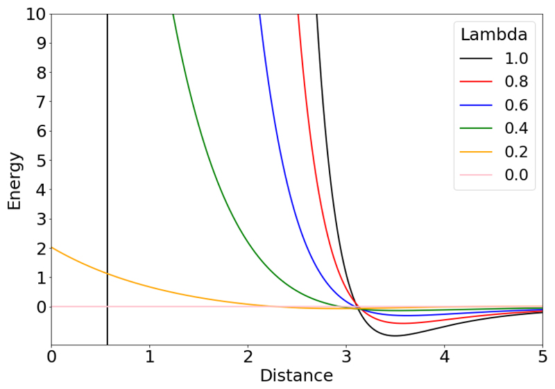
Evidently, if Equation (6) was used from the beginning then the hybrid is redundant and this would be suggested for future work. A plot of Equation (7) for different λ can be seen in Figure (4) below. Equation (7) reduces to Equation (4) when λ = 1 but as λ is perturbed along the alchemical path it behaves like Equation (6) without an exposed singularity, which is crucial for the alchemical calculation.

Figure 4.

Plot of Equation (7) for λ in range 1.0 to 0.0. With ε = 1.0, R_min = 0.35 and γ = 15.

With this functional form implemented into YANK free energy calculations for the Buckingham models could be performed. The alchemical calculations are performed with an identical methodology to the LJ calculations with three free energies calculated and averaged as before and presented in Table (2).

Geometry

To calculate the derivative of the calculated property w.r.t the fitting parameters (needed for the parameter optimization) ForceBalance needs access to the gradient of a snapshot’s energy with respect to the fitting parameters. In this work, this becomes a problem when optimizing the geometry of rigid water molecules as the energy of the system can no longer be considered an explicit function of the geometric parameters [14]. The optimization of geometric parameters is carried out using a trick where all the interaction sites are made into virtual sites during the parameterization calculation only; the parameters defining the virtual site positions are then optimized. Varying these parameters varies the position of the virtual sites and so the position of the interaction sites. Finding the optimal value of these parameters is equivalent to finding the optimal position of the interaction sites. Since we are only concerned with thermodynamic properties the positions of the masses in the molecule are unimportant, but this would affect the fitting of kinetic properties. When optimizing the geometry with the above method the RDFs are calculated from the positions of the virtual interaction sites instead of the positions of the masses. After parametrization the virtual sites are restored to be normal interaction sites but the interaction sites are now in the optimal position determined by the optimization. And therefore, these virtual sites, used for geometry optimization, play no role in the force field after the parametrization.

Scoring

Following the model parameterization, a modified form of the scoring equation proposed by Vega et al. [36] is used in this work to qualitatively compare the relative performance of the water models. Used by Vega and Izadi, [36] [37] this scoring system compares water models and their relative performance at reproducing a variety of bulk properties with experimentally known values. Included in these properties are the height and position of the first OO RDF peak. Efforts are made in the work of Izadi [37] to choose the LJ parameters in a way to maximize the agreement for the position of the first peak and the density. It is then appropriate in their scoring system to consider only the height and position of the first OO RDF peak. In this work, however, an assessment of the agreement for every calculated point for all water RDFs is needed. The first approach to this would be to consider every point in the RDFs in the same way Izadi considers the first OO peak. However, in Vega’s scheme, which takes the maximum of [10 − |(x − x_exp) × 100/(x_exptol)|] and 0, it is possible for models with extremely poor agreement in the RDF over a small r range and good agreement everywhere else to outperform a model which perform with average agreement everywhere. Therefore, a modified method of scoring is presented in Equation (8).

$$Score=\mathit{\text{max}}\left\{\left[10-\frac{{\sum }_n|(x_n-x_n^{\mathit{\text{exp}}})\times 100/(x_n^{\mathit{\text{exp}}}tol)|}{N}\right],0\right\}$$ (8)

The definitions in Equation (8) are like those made in Vega’s work [36] except there is now a summation over n which indexes the non-zero points in the RDF with N as the total number of non-zero points in the RDF. In the case of properties outside the RDFs N would be set, N = 1, and Equation (8) reduces to Vega’s scoring system. This Score will be calculated for the properties and tol values shown in Table (2). For comparison Izadi [37] uses a tol of 0.5 for ρ, H_vap, and position of the first OO peak, 5.0 for the height of the first peak and 2.5 for all other properties. The larger the value of tol the larger the difference between calculated and experimental properties can be before the Score is reduced. The individual Score for each property are averaged to give the final Score.

Results

Lennard-Jones potential

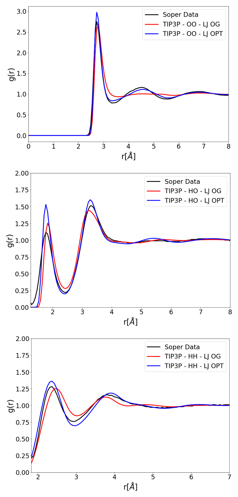
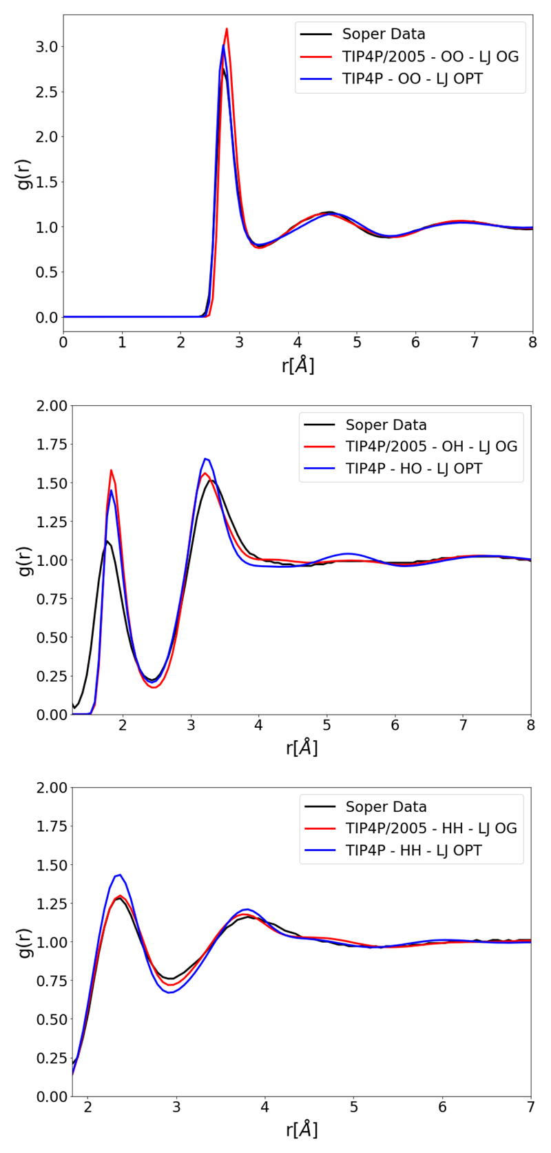
The first section of the results will present the force fields which are using the LJ functional form optimized by RDF fitting. Figure (5), shows the resulting RDFs of an optimization starting from the original TIP3P parametrization. Agreement is improved for all RDFs over the original parametrization. Relative to Figure (2) the under-structuring in the second and third shell of the OO RDF has been reduced; however, this has introduced some over-structuring in the first shell. It will be shown in subsequent sections that this can be treated with the Buckingham potential.

Figure 5.

OO, OH and HH RDFs for an optimized TIP3P type model with a LJ potential (TIP3P-LJ OPT). The parameter set of TIP3P-LJ OPT is parametrized with the fitting procedure shown in this work. Compared to OO, OH and HH RDFs for TIP3P with original parameter set (TIP3P-LJ OG) and experimental Soper data. [17]

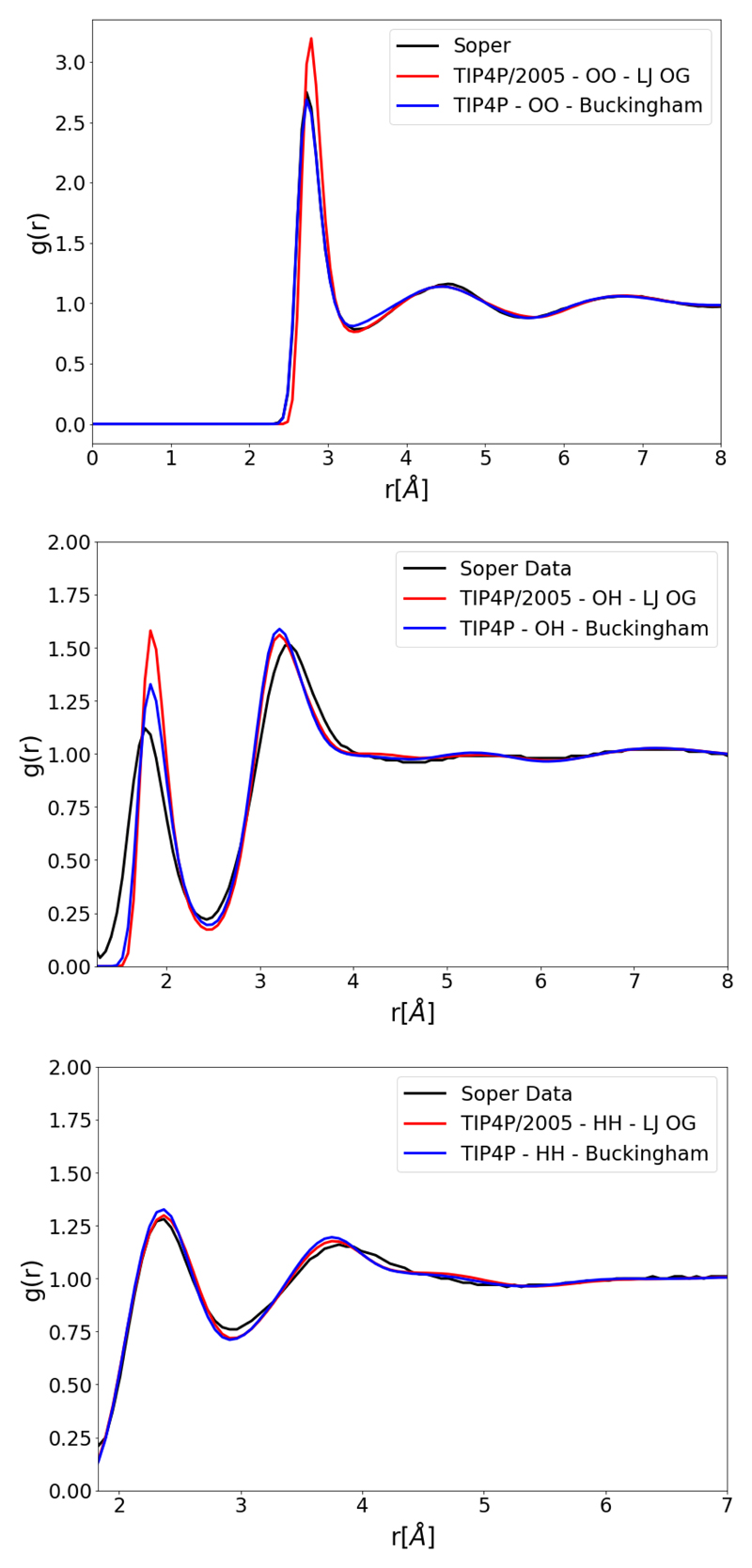
The next set of plots, Figure (6), pertains to the RDF fitting of the TIP4P/2005 model. Compared to the original TIP4P/2005 parametrization, Figure (3) shows that there is an improvement to the OO and OH RDF. The most notable improvement is to the decrease in the over-structuring in the first OO shell which also can be seen as a decrease in the over-structuring of the first OH shell. There is, however, a decrease in the agreement of the HH RDF. The original TIP4P/2005 has a HH RDF which agrees well with experiment. Therefore, the agreement of the HH RDF is likely to worsen as the optimizer attempts to improve the OO RDF whilst sacrificing the HH RDF. This potentially could be fixed by changing the relative weights of the RDFs. Moreover, while the OO over-structuring has decreased it has not been completely resolved.

Figure 6.

OO, OH and HH RDFs for an optimized TIP4P type model with a LJ potential (TIP4P-LJ OPT). The parameter set of TIP4P-LJ OPT is parametrized with the fitting procedure shown in this work. Compared to OO, OH and HH RDFs for TIP4P/2005 with original parameter set (TIP4P-LJ OG) and experimental Soper data. [17]

Buckingham potential

The following section will now consider the use of the Buckingham potential in the currently presented RDF fitting procedure. Here, TIP3P geometry and charges with a Buckingham potential is taken as a starting point. The initial parameters of the Buckingham potential are chosen by hand ensuring the density of the box remains close to 1000 kgm^-3 after equilibration. The results of these optimizations are presented in Figure (7). The under-structuring in the second and third shells is largely resolved, similar to the results in Figure (5); however, now there is also less over-structuring in the first shell. The introduction of the Buckingham potential appears to have made it much easier for these features of the OO RDF to simultaneously agree. All RDF’s MSD are improved by the introduction of the Buckingham potential relative to the original parametrization and to the LJ optimization. Next, the Buckingham potential using TIP4P/2005 geometry and charges are optimized with the result shown in Figure (8). Relative to the optimization using the LJ potential, Figure (6), there is an improvement to all RDFs. Similar to using the Buckingham potential in TIP3P the over-structuring in the first shell can again be reduced. Compared to the original TIP4P/2005, both the OO and OH RDFs significantly improve whilst there is no significant change in HH RDF MSD.

Figure 7.

OO, OH and HH RDFs for an optimized TIP3P type model with a Buckingham potential (TIP3P-Buckingham). The parameter set of TIP3P-Buckingham is parametrized with the fitting procedure shown in this work. Compared to OO, OH and HH RDFs for TIP3P with original parameter set (TIP3P-LJ OG) and experimental Soper data. [17]

Figure 8.

OO, OH and HH RDFs for an optimized TIP4P type model with a Buckingham potential (TIP4P-Buckingham). The parameter set of TIP4P-Buckingham is parametrized with the fitting procedure shown in this work. Compared to OO, OH and HH RDFs for TIP4P/2005 with original parameter set (TIP4P-LJ OG) and experimental Soper data. [17]

The temperature dependence of the densities can be seen in figures S1 and S2 in the supplementary information. Difference plots between the calculated and experimental RDFs are presented in figures S3-S8 in the supplementary information. These highlight the improved RDFs in the majority of cases, particularly the O-O RDF.

Discussion

The improvement to the RDF has been presented in Figures (5-8), but to make a more complete discussion of the presented models, additional relevant properties and all parameters should be inspected. These values are presented in Tables (2) and (3), respectively. Table (2) features the Score as defined in Equation (8) and this is a measure of the relative performance of the presented models. This Score is calculated with the calculated and experimental properties along with the tolerances in in Table (2) using Equation (8). The static dielectric constant ϵ(0), isothermal compressibility κ_T and isobaric heat capacity C_p are calculated by fluctuation formulas in ForceBalance from the same 10 ns trajectory used to calculate the RDFs. The thermal expansion coefficient α_p is calculated following the methodology of Abascal et al [8] performed on seven 0.5 ns simulations being run between 240-360 K. The self-diffusion coefficients D is calculated following the methodology of Horn et al [12] using 20 simulations of 100 ps in an NVE ensemble. µ(D), ϵ(0), D, TMD, ΔG_excess, ΔS_excess, κ_T, C_p and α_p are included in Tables (2) to assess the predictive power of these models, they are properties which were not targeted in the parameter optimization. The poor scoring of TIP3P should be noted; this is a result of the calculations being performed with PME, a scheme for which TIP3P was not parametrized. However, without PME the RDFs remain equally under-structured [4].

Table 3.

Parameters for Original and Re-parametrized Water Models. 3p and 4p Denote Three and Four Point Models. LJ OG Denotes the Original Parametrization. LJ OPT Denotes the LJ Model Optimized in This Work. Buck Denotes the Buckingham Model Optimized in This Work. l₁[Å], l₂[Å], θ° and ϕ° Are the Geometrical Parameter Referenced in Figure (1) and q[e] Is the Oxygen Charge or Virtual Site Charge Again Referenced in Figure (1).

	3P - LJ OG	3P - LJ OPT	3P - Buck	4P - LJ OG	4P - LJ OPT	4P - Buck
𝜖[kcal/mol]	-0.1521	-0.1556	-0.1849	-0.1852	-0.1313	-0.1978
Rmin[Å]	3.5358	3.5335	3.5373	3.5457	3.5584	3.5764
𝛾	N/A	N/A	15.05	N/A	N/A	14.12
q[e]	-0.8340	-0.8506	-0.8189	-1.1128	-0.9824	-1.0828
l1[Å]	0.9572	0.9899	1.0284	0.9572	0.9116	0.9251
𝜃°	104.52	114.13	109.28	104.52	118.00	109.93
𝜙°	N/A	N/A	N/A	120.79	119.44	120.51
l2[Å]	N/A	N/A	N/A	0.1558	0.0133	0.0982

It is clear from looking at the calculated properties in Table (2) that the fitting for TIP3P improves overall agreement with experiment. Relative to the original, TIP3P, parametrization optimizing the LJ potential improves the prediction for D, TMD, ΔG_excess, ΔS_excess, κ_T, C_p and α_p. However, accuracy is lost for ϵ(0) and µ(D). TIP3P-Buckingham corrects this loss of accuracy in ϵ(0) and µ(D) and further adds to the predictive power of the model. Compared to the LJ optimization the Buckingham optimization has improved predictions for µ(D), ϵ(0), D, TMD, ΔG_excess, ΔS_excess, κ_T, C_p and α_p. The TIP3P-Buckingham force field also has the best agreement for the fitted properties ρ, ΔH_excess and all RDF MSDs of any of the TIP3P models presented here.

The LJ optimization in the case of TIP4P/2005 only demonstrates an improved prediction for the calculated value of ΔS_excess but generally sees improved accuracy for the fitted properties OO-MSD, OH-MSD and ΔH_excess. This is perhaps not surprising considering that the TIP4P/2005 parameters have already been carefully optimized to reproduce temperature-dependent and phase change properties. On the other hand, the usefulness of the Buckingham potential is more clearly demonstrated. Compared to TIP4P/2005, the Buckingham model has equivalent or improved predictions for κ_T, ΔG_excess and ΔS_excess but reduced accuracy for µ(D), ϵ(0), D, TMD, C_p and α_p. Of the fitted properties, improved accuracy is seen for OO-MSD, OH-MSD and ΔH_excess and in general overall agreement with experiment is improved, reflected by the higher Score of TIP4P-Buckingham. The reduction in accuracy for TMD, C_p and α_p should not detract from the utility of the Buckingham potential, as no effort was made to fit to any temperature dependent properties in this work. Relative to the optimized LJ model, TIP4P-Buckingham has improved predictions for µ(D), ϵ(0), D, TMD, ΔG_excess, ΔS_excess, κ_T, C_p and α_p; for the fitted properties, improvement is seen for all RDF MSDs and ΔH_excess. In the case of both TIP4P-Buckingham and TIP3P-Buckingham the predicted isothermal compressibility is closer to experiment than original and optimized LJ models, which may reflect the physically motivated repulsive part of the Buckingham potential.

Adding the Buckingham potential with TIP4P/2005 improves overall agreement between the calculated and experimental properties examined in this work. However, the improvement is less definitive compared to using the Buckingham potential in TIP3P, particularly for temperature dependent properties. As a more stringent test of the usefulness of the Buckingham potential, we suggest that the TIP4P/2005 optimization could be reproduced, but using the Buckingham potential instead of LJ. Any improvement or lack thereof in this parametrization would be a good assessment of the Buckingham potentials utility in four-point models.

Of main interest to this work was correcting the over and under-structuring in the OO RDF. It can be seen in Table (2) that both RDF fitting and the use of the Buckingham potential are effective tools to treat this. Using RDF fitting, 85 and 87 percent reductions to the OO MSD are achieved for TIP3P and TIP4P/2005 respectively. When the LJ potential in the TIP3P and TIP4P/2005 models are replaced with a Buckingham potential and optimized targeting the RDF, the MSD in the OO RDF are reduced by 93 and 98 percent, for TIP3P and TIP4P/2005 respectively. It can be seen in Table (2) that this increased agreement for the RDFs has translated into improved predictions of ΔS_excess. In the case of TIP3P the correction of the under structuring in the O-O RDF has increased the correlation in the water and reduced the error in the entropy from 11% to 3%. For TIP4P/2005 the correction of the over structuring in the O-O RDF has reduced the correlation in the water and reduced the error in the entropy from 11% to 2%. Both the three and four-point models using the Buckingham potential have ΔS_excess which agree most closely with experiment compared to the other models examined here.

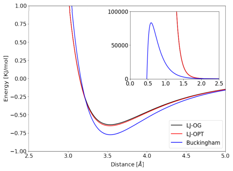
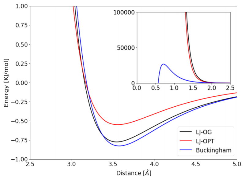
Figures (9) and (10) show comparisons of the LJ and Buckingham potentials using the parameters from Table (3). From Figures (9) and (10) it can be seen that for small atomic separation the Buckingham potential is less repulsive than both original and optimized LJ parametrizations. In the case of TIP3P the original and optimized potential are very similar. The plotted lines practically overlap on the presented scales. These results indicate that the improved agreement of the RDFs using the Buckingham potential is likely to result from the reduced repulsiveness.

Figure 9.

Comparison of non-Coulombic contribution to the potentials of TIP3P type models. The distance referenced here is the interatomic distance between oxygen atoms. LJ-OG as the original parametrization, LJ-OPT as the optimized model presented in this work using the LJ potential and Buckingham as the optimized model presented in this work using the Buckingham potential. Inset shows potentials plotted on larger scale to highlight change in repulsiveness.

Figure 10.

Comparison of non-Coulombic contribution to the potentials of TIP4P type models. The distance referenced here is the interatomic distance between oxygen atoms. LJ-OG as the original parametrization, LJ-OPT as the optimized model presented in this work using the LJ potential and Buckingham as the optimized model presented in this work using the Buckingham potential. Inset shows potentials plotted on larger scale to highlight change in repulsiveness.

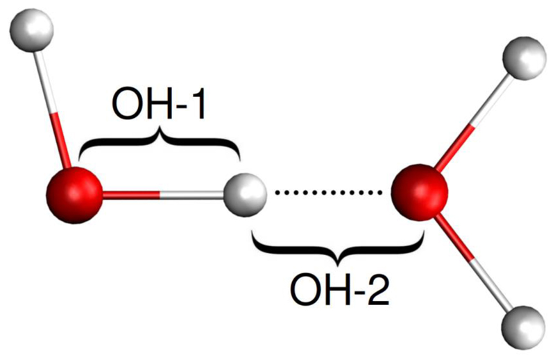
The other trend that can be commented on in these optimizations is the change in the HOH angle. The optimized LJ models favor large HOH angles of between 114° and 118° whereas the angles obtained in Buckingham optimizations are between 108.89° and 109.93°. The angles obtained in the Buckingham optimization are far closer to the tetrahedral angle 109.47°. The change to the bond length can be classified by number of sites modelled where TIP3P models favor longer bonds of approximately 0.99 - 1.03Å and the TIP4P models favor shorter bonds 0.91-0.93 Å. Whilst progress has been made in correcting the over-structuring in the first OO shell, one problem with the current models is that none of them agree well for the second OH shell, presented as the first peak in all OH RDF plotted in this work. When moving from TIP4P/2005 to TIP4P-Buckingham there is a reduction in peak height associated with the OH second shell so that it is closer to the Soper data [17]; this should be expected as in a hydrogen bonding configuration the OO first neighbor and OH second neighbor distances are strongly linked, see Figure (11). Since the OO first shell is now better agreed in TIP4P-Buckingham but the error in the OH second shell persists perhaps the over-structuring in the OH second shell comes from some another source with the first OH shell as a potential candidate.

Figure 11.

Simplification of hydrogen bond in water to the link between OH first, OH-1, and second, OH-2, neighbour distances. It can also be seen that the OO first neighbour (the distance between the two red oxygen atoms) and OH-2 second neighbour are in line. Hydrogen is shown in white.

The nearest-neighbor peak is omitted in the OH and HH RDFs in this work, and if plotted would each feature an infinitely sharp peak corresponding to the OH and HH separations within the molecule respectively. When in a hydrogen bonding configuration, the OH first and second neighbor distances are also highly correlated (see Figure (11)). If the distribution of first OH neighbor distances is unphysically localized due to the rigid bond approximation, this localization could be inherited by the second OH neighbor distance. It might be expected that for non-rigid models the problem would be alleviated; however, this is not the case in common flexible models SPC/Fw [38] and uAMOEBA [39]. Whilst the source of this error has not been treated in this work, a potential source has been speculated upon and a potential solution will be commented on in the conclusion.

It is demonstrable that the Buckingham potential improves the accuracy for many of water’s computed properties, but this should not come as a surprise. The repulsive component of the LJ is chosen partly for computational convenience and it would be hoped that moving towards a more accurate physical description of the repulsion would yield improved computational properties. Previous work has demonstrated that replacing the LJ r⁻¹² term with r⁻⁹ also has the potential for improved accuracy [40]. The remaining open question is if this loss of computational convenience is justified by the gain in accuracy. To answer this an estimation for the computational speed of both the Buckingham and LJ potentials used in three and four site models across several computational platforms can be seen in Table (4). The [ns/day] calculations in Table (4) are performed for a 30 ų box of water with hardware and software configuration provided in the SI. For calculations on GPU platforms (CUDA or OpenCL), the use of Buckingham potentials instead of LJ incurs a small additional cost, resulting in a <10% performance decrease for CUDA (the fastest platform overall). This is less expensive than adding an interaction site (i.e. going from TIP3P to TIP4P) which results in a 20% overall performance decrease. On the other hand, the CPU platform is not well-optimized for the Buckingham potential, as the performance decreases by 90% relative to LJ. As such the Buckingham potential could be considered in place of or supplementary to adding additional interaction sites.

Table 4.

Comparison of ns/day Performance Between: Lennard-Jones (LJ) and Buckingham (Buck) Functional forms, Three (3p) and Four-Point (4p) Models and Computational Platforms. Nvidia Quadro M1000M (CUDA, OpenCL). Intel i5-6300HQ (CPU).

	3P – LJ [ns/day]	3P – Buck [ns/day]	4P – LJ [ns/day]	4P – Buck [ns/day]
CUDA	203	189	169	142
OpenCL	150	133	121	97
CPU	47	5	30	3

Conclusion

The present work sought to improve the structural properties of water models. This was achieved by addition of the RDF as a target property to ForceBalance, a code for the systematic optimization of force fields. Fitting with the OO, OH and HH experimental RDFs was carried out starting from the TIP3P and TIP4P/2005 water models. Re-parametrizations were performed which overall achieved improved structural properties, but these models still carried some over-structuring in the first OO RDF shell. To treat this, the LJ potentials in the models were replaced with Buckingham potentials and these new models were again parametrized targeting the RDFs. The new Buckingham based models were found to have the best agreement with the experimental RDFs. TIP3P–Buckingham, a new three-site model, achieved a reduction of 93, 47 and 57 percent to the OO, OH and HH RDF MSDs respectively when compared to TIP3P. TIP4P-Buckingham, a new four-site model, reached the best agreement for the OO RDF out of all the models tested here with reductions of 98 and 44 percent for the OO and OH RDF MSDs respectively but a percentage increase of 20 for the HH RDF MSD when compared to TIP4P/2005. This improvement to the RDFs MSD was reflected in ΔS_excess where the percentage error in ΔS_excess for TIP3P-Buckingham and TIP4P-Buckingham was 2 and 3 percent respectively compared to 11 percent in both TIP3P and TIP4P/2005.

In validation studies it was demonstrated that these Buckingham models improve many non-targeted properties. This improvement was particularly pronounced for TIP3P-Buckingham which was demonstrated to have equal or greater accuracy for all non-fitted properties calculated in this work when compared to both the original and optimized LJ TIP3P models. Of the four-point models the optimized LJ model (TIP4P-LJ OPT) achieved improved accuracy for ΔS_excess when compared to TIP4P/2005 where as TIP4P-Buckingham displayed improved or equal predictive power for κ_T, ΔG_excess and ΔS_excess when compared to TIP4P/2005. TIP4P-Buckingham had more accurate calculations for all non-targeted properties when compared to TIP4P-LJ OPT.

The above improvements to both fitted and predicted properties demonstrates the utility of the Buckingham potential, with TIP3P-Buckingham equalling or improving the accuracy of the entire property set studied here compared to TIP3P and TIP4P-Buckingham achieving improved accuracy, where a LJ optimization could not, when compared to TIP4P/2005. Overall, the TIP3P-Buckingham performs best achieving the highest Score in a modified version of Vega’s scoring system [36] of any models tested in this work. This is particularly promising considering the small additional cost of replacing LJ with a Buckingham potential on modern GPU hardware. TIP4P-Buckingham achieved the highest Score of the presented TIP4P models, however, this came at the sacrifice of some of the non-targeted properties. A methodology was outlined in the discussion that could more rigorously compare a four-point Buckingham model to TIP4P/2005.

An accurate representation of the intermolecular geometry of water molecules is important to generate accurate thermodynamic properties [41] [42]. The optimized Buckingham potentials are less repulsive than both the original and optimized LJ potentials, in agreement with predictions that the LJ potential is too repulsive [24]. This work could be extended by investigating the source of the error in the second OH peak; this may be addressable by using a flexible water model and specifically fitting the OH RDF. In the optimization of the models presented here, a methodology has been described which can systematically fit computational to experimental RDFs. This general methodology is expected to be highly applicable to other molecular liquids. In this work progress has been made to addressing the under- and over-structuring of the water OO RDF and improvements in ΔS_excess seen. However, considering the work of Lazaridis et al, [11] the important orientational contribution to the total entropy is not targeted. To address this the excess free energy could be made a target of the parameterization; if the excess enthalpy were also targeted, it would make the excess entropy an implicit target of the parameterization. A major challenge would be the sampling time required to calculate converged values for the excess free energy changes, especially in the context of an iterative optimization. One promising possibility would be to employ a perturbative methodology to compute the free energy change from the original force field to the current set of parameter values being optimized; this would remove the requirement of running a free energy calculation at every optimization cycle, and by extension allow the excess entropy to be implicitly targeted.

Supplementary Material

Density curves and RDF difference plots for the water models discussed in the paper. Details of the free energy calculations performed. Details of the computational performance for the water models discussed in the paper.

References

- (1).Soper AK, Silver R. Hydrogen-Hydrogen Pair Correlation Function in Liquid Water. Phys Rev Lett. 1982;49:471–474. [Google Scholar]
- (2).Bernal J, Fowler R. A Theory of Water and Ionic Solution, with Particular Reference to Hydrogen and Hydroxyl Ions. J Chem Phys. 1933;1:515–548. [Google Scholar]
- (3).Jorgensen WL. Quantum and Statistical Mechanical Studies of Liquids.10. Transferable Intermolecular Potential Functions for Water, Alcohols, and Ethers. Application to Liquid Water. J Am Chem Soc. 1981;103:335–340. [Google Scholar]
- (4).Jorgensen WL, Chandrasekhar J, Madura JD, Impey RW, Klein ML. Comparison of Simple Potential Functions for Simulating Liquid Water. J Chem Phys. 1983;79:926–935. [Google Scholar]
- (5).Price DJ, Brooks CL. A Modified TIP3P Water Potential for Simulation with Ewald Summation. J Chem Phys. 2004;121:10096–10103. doi: 10.1063/1.1808117. [DOI] [PubMed] [Google Scholar]
- (6).Jorgensen WL, Madura JD. Temperature and Size Dependence for Monte Carlo Simulations of TIP4P Water. Mol Phys. 1985;56:1381–1392. [Google Scholar]
- (7).Wu Y, Tepper HL, Voth GA. Flexible Simple Point-Charge Water Model with Improved Liquid-State Properties. J Chem Phys. 2006;124:024503. doi: 10.1063/1.2136877. [DOI] [PubMed] [Google Scholar]
- (8).Abascal JL, Vega C. A General Purpose Model for the Condensed Phases of Water: TIP4P/2005. J Chem Phys. 2005;123:234505. doi: 10.1063/1.2121687. [DOI] [PubMed] [Google Scholar]
- (9).Gilson MK, Zhou H-X. Calculation of Protein-Ligand Binding Affinities. Ann Rev Biophys. 2007;36:21–42. doi: 10.1146/annurev.biophys.36.040306.132550. [DOI] [PubMed] [Google Scholar]
- (10).Levy Y, Onuchic JN. Water Mediation in Protein Folding and Molecular Recognition. Annu Rev Biophys Biomol Struct. 2006;35:389–415. doi: 10.1146/annurev.biophys.35.040405.102134. [DOI] [PubMed] [Google Scholar]
- (11).Lazaridis T, Karplus M. Orientational Correlations and Entropy in Liquid Water. J Chem Phys. 1996;105:4294–4316. [Google Scholar]
- (12).Horn HW, Swope WC, Pitera JW, Madura JD, Dick TJ, Hura GL, Head-Gordon T. Development of an Improved Four-Site Water Model for Biomolecular Simulations: TIP4P-EW. J Chem Phys. 2004;120:9665–9678. doi: 10.1063/1.1683075. [DOI] [PubMed] [Google Scholar]
- (13).Wang L-p, Head-gordon T, Ponder JW, Ren P, Chodera JD, Eastman PK, Martinez TJ, Pande VS. Systematic Improvement of a Classical Molecular Model of Water. J Phys Chem B. 2013;117:9956–9972. doi: 10.1021/jp403802c. [DOI] [PMC free article] [PubMed] [Google Scholar]
- (14).Wang L-p, Martinez TJ, Pande VS. Building Force Fields: An Automatic, Systematic, and Reproducible Approach. J Phys Chem Lett. 2014;5:1885–1891. doi: 10.1021/jz500737m. [DOI] [PMC free article] [PubMed] [Google Scholar]
- (15).Levine BG, Stone JE, Kohlmeyer A. Fast Analysis of Molecular Dynamics Trajectories with Graphics Processing Units-Radial Distribution Function Histogramming. J Comput Phys. 2011;230:3556–3569. doi: 10.1016/j.jcp.2011.01.048. [DOI] [PMC free article] [PubMed] [Google Scholar]
- (16).Gray CG, Gubbins KE. Theory of Molecular Fluids: Volume 2: Applications. Oxford University Press; 1984. p. 628. [Google Scholar]
- (17).Soper AK. The Radial Distribution Functions of Water and Ice from 220 to 673 K and at Pressures up to 400 MPa. Chem Phys. 2000;258:121–137. [Google Scholar]
- (18).Hernando JA. Thermodynamic Potentials and Distribution Functions. Mol Phys. 1990;69:319–326. [Google Scholar]
- (19).Laird BB, Haymet ADJ. Calculation of the Entropy of Binary Hard Sphere Mixtures From Pair Correlation Functions. J Chem Phys. 1992;97:2153–2155. [Google Scholar]
- (20).Huggins DJ. Correlations in Liquid Water for the TIP3P-Ewald, TIP4P-2005, TIP5P-Ewald, and SWM4- NDP Models·. J Chem Phys. 2012;136:064518. doi: 10.1063/1.3683447. [DOI] [PMC free article] [PubMed] [Google Scholar]
- (21).Soper AK. Orientational Correlation Function for Molecular Liquids: the Case of Liquid Water. J Chem Phys. 1994;101:6888–6901. [Google Scholar]
- (22).Rick SW. A Reoptimization of the Five-Site Water Potential (TIP5P) for use with Ewald Sums. J Chem Phys. 2004;120:6085–6093. doi: 10.1063/1.1652434. [DOI] [PubMed] [Google Scholar]
- (23).Abascal JLF, Sanz E, Fernández RG, Vega C. A Potential Model for the Study of Ices and Amorphous Water: TIP4P/Ice. J Chem Phys. 2005;122:234511. doi: 10.1063/1.1931662. [DOI] [PubMed] [Google Scholar]
- (24).Soper AK. Joint Structure Refinement of X-ray and Neutron Diffraction Data on Disordered Materials: Application to Liquid Water. J Phys: Condens Matter. 2007;19:335206. doi: 10.1088/0953-8984/19/33/335206. [DOI] [PubMed] [Google Scholar]
- (25).Wheatley RJ, Price SL. An Overlap Model for Estimating the Anisotropy of Repulsion. Mol Phys. 1990;69:507–533. [Google Scholar]
- (26).Buckingham R. The Present Status of Intermolecular Potentials for Calculations of Transport Properties. Planet Space Sci. 1961;3:205–216. [Google Scholar]
- (27).Wang L-p, Chen J, Voorhis TV. Systematic Parametrization of Polarizable Force Fields from Quantum Chemistry Data. J Chem Theory Comput. 2013;9:452–460. doi: 10.1021/ct300826t. [DOI] [PubMed] [Google Scholar]
- (28).Eastman P, Friedrichs MS, Chodera JD, Radmer RJ. OpenMM 4: A Reusable, Extensible, Hardware Independent Library for High Performance Molecular Simulation. J Chem Theory Comput. 2012;9:461–469. doi: 10.1021/ct300857j. [DOI] [PMC free article] [PubMed] [Google Scholar]
- (29).McGibbon RT, Beauchamp KA, Harrigan MP, Klein C, Swails JM, Hernandez CX, Schwantes CR, Wang L-P. MDTraj: A Modern Open Library for the Analysis of Molecular Dynamics Trajectories. Biophys J. 2015;109:1528–1532. doi: 10.1016/j.bpj.2015.08.015. [DOI] [PMC free article] [PubMed] [Google Scholar]
- (30).Cooper J, London EN, Dooley R. International Association for the Properties of Water and Steam. 2007. [Google Scholar]
- (31).Rizzi A, Grinaway PB, Parton DL, Shirts MR, Wang K, Eastman P, Friedrichs M, Pande VS, Branson K, Mobley DL, Chodera JD. YANK: A GPU-Accelerated Platform for Alchemical Free Energy Calculations. [Internet] http://getyank.org.
- (32).Chodera JD, Shirts MR. Replica Exchange and Expanded Ensemble Simulations as Gibbs Sampling: Simple Improvements for Enhanced Mixing. J Chem Phys. 2011;135:194110. doi: 10.1063/1.3660669. [DOI] [PubMed] [Google Scholar]
- (33).Shirts MR, Chodera JD. Statistically optimal analysis of samples from multiple equilibrium states. J Chem Phys. 2008;129:124105. doi: 10.1063/1.2978177. [DOI] [PMC free article] [PubMed] [Google Scholar]
- (34).Chodera JD, Rizzi A, Naden L, Beauchamp K, Grinaway PB, Fass J, Rustenburg B, Ross GA, Simmonett A, Swenson DWH. OpenMMTools 0.15.0. doi: 10.5281/zenodo.1205753. [Internet] [DOI] [Google Scholar]
- (35).Shirts MR, Mobley DL, Chodera JD. Alchemical Free Energy Calculations: Ready for Prime Time? Annu Rep Comput Chem. 2007;3:41–59. [Google Scholar]
- (36).Vega C, Abascal LF. Simulating Water with Rigid Non-Polarizable Models: A General Perspective. RSC Adv. 2011;13:19663–19688. doi: 10.1039/c1cp22168j. [DOI] [PubMed] [Google Scholar]
- (37).Izadi S, Anandakrishnan R, Onufriev AV. Building Water Models: A Different Approach. J Phys Chem Lett. 2014;5:3863–3871. doi: 10.1021/jz501780a. [DOI] [PMC free article] [PubMed] [Google Scholar]
- (38).Lamoureux G, MacKerell A, Roux B. A Simple Polarizable Model of Water Based on Classical Drude Oscillators. J Chem Phys. 2003;119:5185–5197. [Google Scholar]
- (39).Qi R, Wang LP, Wang Q, Pande VS, Ren P. United Polarizable Multi-Pole Water Model for Molecular Mechanics Simulation. J Chem Phys. 2015;143:014504. doi: 10.1063/1.4923338. [DOI] [PMC free article] [PubMed] [Google Scholar]
- (40).Te JA, Ichiye T. Temperature and Pressure Dependence of the Optimized Soft-Sticky Dipole-Quadrupole-Octupole Water Model. J Chem Phy. 2010;132:114511. doi: 10.1063/1.3359432. [DOI] [PMC free article] [PubMed] [Google Scholar]
- (41).Huggins DJ. Estimating translational and orientational entropies using the k-nearest neighbors algorithm. J Chem Theory Comput. 2014;10:3617–3625. doi: 10.1021/ct500415g. [DOI] [PubMed] [Google Scholar]
- (42).Huggins DJ. Benchmarking the thermodynamic analysis of water molecules around a model beta sheet. J Comp Chem. 2012;33:1383–1392. doi: 10.1002/jcc.22971. [DOI] [PMC free article] [PubMed] [Google Scholar]
Associated Data
This section collects any data citations, data availability statements, or supplementary materials included in this article.