Reduction of All-Atom Protein Folding Dynamics to One-Dimensional Diffusion

Abstract

Theoretical models have often modeled protein folding dynamics as diffusion on a low-dimensional free energy surface, a remarkable simplification. However, the accuracy of such an approximation and the number of dimensions required were not clear. For all-atom folding simulations of ten small proteins in explicit solvent we show that the folding dynamics can indeed be accurately described as diffusion on just a single coordinate, the fraction of native contacts (Q). The diffusion models, parametrized reproduce both folding rates, and finer details such as transition-path durations and diffusive propagators. The Q-averaged diffusion coefficients decrease with chain length, as anticipated from energy landscape theory. Although the Q-diffusion model does not capture transition-path durations for the protein NuG2, we show that this can be accomplished by designing an improved coordinate Q_opt. Overall, onedimensional diffusion on a suitable coordinate turns out to be a remarkably faithful model for the dynamics of the proteins considered.

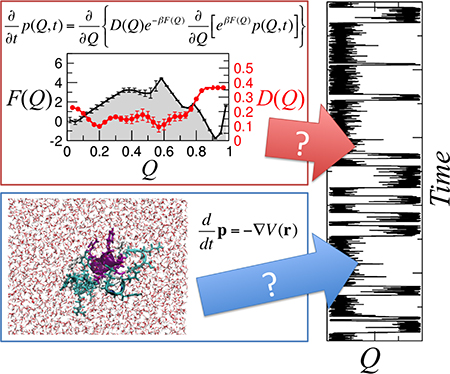
Graphical Abstract

Introduction

Theory and simulations of simplified models have yielded many insights into protein folding dynamics. In particular, the energy landscape framework^1–3 has proved successful in explaining a wide range of experimental observations, starting from the hypothesis that the energy landscape of natural protein sequences is “funneled” toward the native structure. Examples include the relative folding rates of two-state proteins near their transition midpoints,⁴ prediction of folding mechanism and folding ϕ-values,⁵ the mechanism of protein-protein association,⁶ coupled folding-binding,⁷ domain swapping⁸ and domain-swapped misfolding^9,10 and the effect of a tensile force on protein folding.^11,12 Since comparison with experimental observations is the true test of any theory, the above examples provide compelling support for a funneled folding energy landscape.

Nonetheless, any theoretical model of a process as complex as protein folding requires well-chosen simplifying assumptions. There are two such key simplifications in energy landscape theory.^13,14 The first is that the folding energy landscapes of naturally occurring proteins are designed so that the influence of non-native interactions is minimized (known as the “principle of minimal frustration”¹³). This leads to free energy landscapes which are “funneled” toward the native state,¹⁵ so that lower energy is associated with increasing similarity to the native state. In order to describe folding dynamics on the funneled energy landscape, a second simplification was also introduced, namely that motion along this coordinate was Markovian, and could be described as diffusion on the corresponding free energy surface.¹⁴ This formed the basis of a theory for computing diffusion coefficients and folding rates based on the statistical properties of the landscape¹⁴ (although non-Markovian effects have also been considered¹⁶).

The availability of detailed all-atom simulations of protein folding at equilibrium has now made it possible to test the assumptions of energy landscape theory directly. We have recently tested the first using simulations of a set of ten small proteins studied by Shaw and co-workers,^17–19 for which folding was barrier-limited. We found that for all the naturally occurring proteins in the data set, folding mechanism was defined by native contacts, with little role for non-native interactions,²⁰ consistent with the results of earlier lattice-model studies.²¹ The single exception was for a designed protein α₃D, in which non-native salt bridges introduced some frustration on folding transition paths, recently also probed experimentally.²² The above assumption allows for a simplified description of protein folding energy landscapes, and supports the class of computational models in which only native interactions are favourable^5,23–26 (Gō models ²⁷). It also helps to explain why reaction coordinates measuring similarity to the native state, such as the fraction of native contacts, Q,²⁸ are able to capture folding barriers and mechanisms.

The second simplification, namely that diffusion in a low-dimensional space can capture protein folding dynamics, has relevance beyond its role in theoretical protein folding models. This is because diffusive models for reaction dynamics such as Kramers theory²⁹ are frequently used to describe folding dynamics and rates in experiments.^30–34 The assumption of diffusive dynamics has been tested against both lattice models^35,36 and off-lattice Gō models, ³⁷ showing that for these simplified systems, the diffusive picture holds rather well. However, all-atom models including explicit solvent have orders of magnitude more degrees of freedom and consequently more complex energy landscapes. Therefore, it is important also to test how well the above assumption holds for folding of these more realistic models.

Here, we consider the question: how faithfully can the folding dynamics of all-atom unbiased MD simulations by Shaw and co-workers^17–19 be captured with a one-dimensional (1D) diffusion model? We use a Bayesian procedure to determine the 1D free energy surface and diffusion coefficients which best capture the local dynamics on this landscape.^37–40 We find that the folding and unfolding rates of the proteins are very well described by these diffusion models. In addition to capturing folding rates, which mainly reflect long-time dynamics, we find that we can also reproduce the duration of transition paths, which occur over a much shorter time scale. Thus, diffusion on the fraction of native contacts Q appears to be a remarkably good model for folding dynamics. Since diffusion in a low dimensional space is often used in interpreting physical experiments on folding dynamics,^32,34 we have also investigated the dependence of the 1D landscape parameters on protein properties. We find little correlation of barrier heights with protein size (as perhaps expected). More interestingly, the barrier curvatures on Q are almost invariant across the set of proteins studied, but diffusion coefficients on Q decrease with increasing chain length, consistent with the predictions of landscape theory.

Methods

Diffusion model

The one-dimensional diffusion model was fitted using a previously described Bayesian procedure^37–40 in which the propagators p(Q_j,t + ∆t,Q_i,t) from the discretized diffusion model were used as a likelihood function for the observed statistics of transitions between bins in Q after a lag time t, thus the log-likelihood is given by

$$L=p(\text{data}|\left\{D_i\right\},\left\{F_i\right\})={\displaystyle \prod _{i,j}{\left[p\left(Q_j,t+\Delta t|Q_i,t\right)\right]}^{N_{ji}}}$$ (1)

where N_ji is the number of observations within bin Q_j a time ∆t after an observation in bin Q_i in the simulation. A smoothness prior of the form p({D_i}) = П_i exp[−(D_i−D_i+1)²/(γ² min(D_i,D_i+1)²)] was used. Here, the stiffness parameter γ = 0.02 reflects our expectation that adjacent discretized diffusion coefficients D_i,D_i+1 should be similar. Thus the posterior distribution was obtained from Monte Carlo sampling of

$$p\left(\left\{D_i\right\},\left\{F_i\right\}|\text{ data }\right)\propto p(\text{ data }|\left\{D_i\right\},\left\{F_i\right\})p\left(\left\{D_i\right\}\right)$$ (2)

Further details are given in Ref.³⁸ In Fig. S1, we show the sensitivity of the resulting positiondependent diffusivity profile D(Q) to the the value of γ. The final value selected was chosen to be the smallest which would not appreciably decrease the likelihood of the diffusion model; thus we aim to select from the possible models with similar likelihood that which has the smoothest D(Q) profile.

Errors on diffusion coefficients and free energies were estimated by block analysis.⁴¹

Brownian Dynamics

We use the Ermak-McCammon algorithm⁴² to simulate Brownian dynamics in one dimension. For position-dependent diffusion coefficients D(Q) and free energies βF(Q), the position update after time step ∆t can be written as

$$Q_{t+\Delta t}=Q_t+\frac{dD\left(Q_t\right)}{dQ}\Delta t-\beta \frac{dF\left(Q_t\right)}{dQ}D\left(Q_t\right)\Delta t+R(t)$$ (3)

where Q_t and Q_t+∆t are the positions at times t and t + ∆t, and R(t) is a random displacement chosen from a Gaussian distribution with zero mean and variance 2D∆t. A time step of 0.1 ns was used.

Reaction Coordinate Optimization

We have shown in a previous publication⁴³ that, p(TP|Q), which is the probability of being on a transition path given that the system is at Q, should have a single sharp peak, for a two-state reaction on a good reaction coordinate Q. Using Bayes theorem, p(TP|Q) can be written as

$$p(\text{TP}|Q)=\frac{p(Q|\text{TP})p(\text{TP})}{p_{\text{eq}}(Q)}$$ (4)

where p_eq(Q) and p(Q|TP) are the probability densities on Q of the equilibrium ensemble and the transition path ensemble, respectively. Both can be calculated from histogramming the MD trajectories. To improve the reaction coordinate Q, we optimize the maximum of a Gaussian fit to p(TP|Q) to ensure that all configurations on the transition paths are condensed into a single sharp peak in p(TP|Q). We use a Monte Carlo optimization procedure in which we modify the relative weights w_i in Q (Eq. 8) in three different ways: randomly changing the weight w_i, swapping the weights w_i and w_j, and reversing the sign of the weight w_i. We estimate the projections of the trajectories on a trial coordinate Q’ and accept only moves that increase the maximum of the Gaussian fit to p(TP|Q’). We apply this procedure iteratively to obtain an optimal w_opt, which gives a sharply peaked distribution of P(TP|Q_opt).

Landscape parameters

We define the Q-averaged diffusion coefficient D_c as:

$$D_c^{-1}=\frac{{\displaystyle {\int }_{Q_{\text{u}}}^{Q_f}\exp }[\beta F(Q)]D{(Q)}^{-1}dQ}{{\displaystyle {\int }_{Q_{\text{u}}}^{Q_f}\exp }[\beta F(Q)]dQ}$$ (5)

where the integral is performed between the unfolded and folded minima on Q, Q_u and Q_f.

Barrier heights for folding and unfolding are determined from the difference between the maximum free energy on the barrier and the minimum in each basin. Stabilities were obtained from

$$\Delta G_{\text{f}-\text{u}}=-k_{\text{B}}T\ln \left[{\displaystyle {\int }_{‡}^1\exp }[-F(Q)]dQ/{\displaystyle {\int }_0^{‡}\exp }[-F(Q)]dQ\right]$$ (6)

Curvatures of stables states u,f and barriers ‡ are determined from:

$${\omega }_{\text{s}}^{-1}\approx \frac{1}{\sqrt{2\pi }}{\displaystyle {\int }_{\text{S}}\exp }\left[\lambda \left(F\left(Q_{\text{s}}\right)-F(Q)\right)\right]dQ$$ (7)

where s ∈ {u,f,‡}, Q_s is the location of s on Q, λ = 1 for u and f, and λ = −1 for ‡.

Results and Discussion

We consider as a reaction coordinate the fraction of native contacts²⁸ Q(x) formed in a given configuration x (Eq. 8). This coordinate has already been shown to be a good folding coordinate in several studies,^37,43,44 including for the set of all-atom protein simulations considered here,²⁰ in the sense that it is able to discriminate folding transition states from other non-reactive states.⁴⁵ In supporting Fig. S2, we show a Bayesian criterion for reaction coordinate quality for each protein. In all cases but one (CLN025), Q is a good coordinate, in the sense the the probability of being on a transition path for a give Q-value, p(TP|Q) has a single peak with a maximum near the theoretical value of 0.5.⁴⁵ However, there is a substantial statistical error on these estimates, due to the limited number of transition paths sampled. We project the all-atom trajectories onto Q, using a common definition of Q for all proteins, as described in our earlier work.²⁰ Our aim is to describe the dynamics using a Smoluchowski diffusion equation ∂_tp(Q,t) = ∂_Q{D(Q)exp(−βF(Q))∂_Q[exp(βF(Q))p(Q,t)]}, parametrized by positiondependent free-energies F(Q) and diffusion coefficients D(Q). The position-dependence of D is a consequence of the projection of the high-dimensional folding dynamics onto a single coordinate, Q. We use a Bayesian procedure to determine the one-dimensional free energies F(Q) and diffusion coefficients D(Q) which best describe the observed simulation data for ten of the proteins studied by Shaw and co-workers^17,19 (full details of the proteins and simulations used are given in Table S1). The optimal free energies and diffusion coefficients are shown in Fig. 1.

Figure 1:

Free energy surfaces and diffusion coefficients. Discretized free energies F(Q) (black curves) and D(Q) (red curves) have been determined using a Bayesian procedure,^38,43 with a lag time of 100 ns, for each of the ten proteins considered. The length of each protein is given in brackets next to its name.

We have selected the ten proteins with a barrier to folding in the simulations^17–19 in order to facilitate comparison between MD and diffusion models for folding and unfolding rates and transition-path durations, the key observable quantities characterizing folding dynamics. An appreciable position-dependence of the diffusion coefficients D(Q) is seen, although the coefficient of variation (defined as σ/μ, where the mean μ and standard deviation σ characterize the distribution of D) is quite modest, in the range of 0.15–0.5 for all proteins. Thus, the position-dependence of D is not expected to have a large influence on the folding dynamics, and should be reasonably approximated by a constant D (see further below).

Diffusion models capture folding dynamics

The parameters presented in Fig. 1 represent the optimal diffusive models for each protein – but how well does each model reproduce dynamics of folding? To answer this question we have performed Brownian dynamics (BD) simulations⁴² using the fitted parameters (Eq. 3). Examples of the trajectories Q(t) obtained from MD and BD are shown in Fig. 2A and 2B for the GTT WW domain. Superficially, the trajectories have rather similar characteristics, and identical free energy surfaces F(Q) as expected. However, there are some small differences, for example fast fluctuations in the unfolded state in the MD simulations which are not present in the BD trajectories, discussed further below. To make a quantitative comparison, we compute three statistics for each protein: the mean first passage time for folding τ_f (average residence time in the unfolded state), the mean first passage time for unfolding τ_u, as well as the mean transition path duration, τ_TP, i.e. the time taken to cross between unfolded and folded (or the reverse). The folding and unfolding times computed from BD simulations are in excellent agreement with those from MD (Fig. 2C). This is an important requirement for the diffusion model to be useful, but not necessarily a strong validation: the model may capture the slow dynamics correctly by virtue of being fitted to pairs of observations separated by long lag times, but describe short-time fluctuations poorly. The transition-path times τ_TP provide a more stringent test, since most of them are not much longer than the lag time of 100 ns used to construct the diffusion models. In addition, transition paths have a special importance since they reflect the parts of the trajectory containing the reaction mechanism.

Figure 2:

Comparison of MD simulations with diffusive dynamics. A: Brownian dynamics (BD) simulations Q(t) using parameters from the 1D diffusion model on Q for the GTT WW domain. The first and second halves of the trajectory are shown as lines and points respectively; the potential of mean force (PMF) is shown on the right. B: Corresponding projection Q(x(t)) of MD trajectories x(t) for GTT WW domain, and PMF on right. C: Folding (blue) and unfolding (green) times from MD simulation compared to those predicted from Brownian dynamics (BD) using the 1D diffusion model. D: Transition-path durations τ_TP for BD and MD compared. The outlier NuG2 is indicated. Orange-filled symbols in (C) and (D) indicate results obtained with the optimized Q_opt coordinate for NuG2. Insets in (C) and (D) compare results obtained with the original diffusion model using position-dependent diffusion coefficients D(Q) and with one using a constant diffusion coefficient, D_c defined in Eq. 5.

Remarkably, we find that the diffusion models also capture very well the transition-path durations (Fig. 2D), which range from approximately 0.1 to 2 μs, only just longer than the lag time used to construct the diffusion model. There is one notable outlier, the NuG2 protein. This corresponds to an engineered variant of protein G⁴⁶ with a further three mutations,¹⁷ which has recently been shown to be a stable two-state folder.⁴⁷ We show in the next section that the reason for this failure is that the vanilla definition of Q is not a sufficiently good reaction coordinate for NuG2.

To determine how important it is to use a position-dependent diffusion coefficient, we have also computed the rates and transition-path durations using a constant diffusion coefficient D_c, derived from the position-dependent diffusion coefficients via Eq. 5 (Insets to Fig. 2C,D). We find that we obtain almost identical folding rates with the position-dependent and constant diffusion coefficients, however this is expected because the diffusion coefficients were averaged in a way which optimizes the calculation of rates. A more sensitive test is again the reproduction of transition-path durations. In this case, some discrepancies are evident, indicating that the use of position-dependent diffusion coefficients can capture details of dynamics better than the constant diffusion coefficient which is optimal for reproducing folding rates. Although it would be possible to instead define a constant diffusion coefficient to fit transition path times, it is clear that it is difficult to reproduce both rates and transition-path times without allowing position-dependent diffusivity.

A last check uses the propagators of the diffusion model, p(Q,t|Q₀,0) which give the probability density on Q, given that the protein was at Q₀ a time t earlier. Comparison of the diffusive propagators with the estimate constructed directly from observations in the MD trajectores provides an even more sensitive and detailed test of the model. In Fig. 3, we compare propagators computed from the diffusion model for ubiquitin with those estimated from MD. For a number of different origins Q₀, we compute the propagators at different lag times t, ranging from 1 ns to 1 μs. At all except the very earliest lag time of 1 ns, we find that the diffusion model propagators agree remarkably well with the simulations. This is true even for a lag of 10 ns, shorter than the 100 ns lag used to fit the diffusion model. The disagreement for very short lags is likely due to short-time memory effects not captured by a diffusion model (and not relevant to the dynamics at longer times), and explains the additional fast fluctuations of Q visible in the unfolded state of the MD, but not in the BD trajectory. The accuracy of the diffusive propagators at intermediate times helps to explain the quality of the transition-path time predictions.

Figure 3:

Diffusive propagators for Ubiquitin. Comparison of propagators p(Q,t|Q₀,0) from the 1D diffusion model (lines) with those estimated directly from MD statistics (symbols). Propagators for lag times of 1 ns, 10 ns, 100 ns and 1 μs are shown in green, black, red and blue respectively (a lag of 100 ns was used to parametrize the diffusion model). The initial positions Q₀ are shown by vertical broken lines in each plot.

Finally, we have also compared the Q correlation functions computed analytically from the diffusion model⁴⁸ with those determined directly from the original trajectories (Fig. S3). In many cases, the relatively small number of transitions make an accurate estimate of the correlation function from the trajectories difficult; however for the proteins which have a large number of folding/unfolding transitions (CLN025, Trp Cage TC10b, NLE Villin), there is a good agreement between the two, further confirming the quality of the diffusion model.

Optimized reaction coordinate for NuG21

The overestimate of the transition-path time from the diffusion model for the variant of protein G, NuG2, (Fig. 2D) might be explained by the quality of vanilla Q as a reaction coordinate. For example, if Q did not separate configurations on the barrier from those which belong in the stable (folded,unfolded) minima, the barrier in F(Q) would appear lower than the true barrier. Then, in order to correctly capture the slow relaxation on Q (i.e. folding/unfolding rates), the diffusion coefficient D(Q) is forced to be too low near the barrier. However, unlike the folding rates which are exponentially sensitive to the barrier height, the transition-path durations depend mainly on the diffusion coefficient and hence will be overestimated.⁴⁹ Although the maximum of the Bayesian criterion for reaction coordinate quality, p(TP|Q), for NuG2 in Fig. S1 does not differ appreciably from many of the other proteins, there is a large statistical error on the estimate of this quantity. In addition, the shape of the function p(TP|Q) is rather lopsided, suggesting the possible existence of an off-pathway intermediate in the barrier region.

We set out to test this hypothesis by optimizing the maximum of a Gaussian fit to p(TP|Q), which is the probability of being on a transition path given that the system is located at position Q, by varying the weights w_i of the N_c native contacts in calculating the fraction of native contacts

$$Q(x)={\displaystyle \sum _{i=1}^{N_c}{w}_i}\frac{1}{1+e^{\beta \left|r_i(x)-\gamma r_i^0\right|}}$$ (8)

where w_i is defined as 1/N_c in the original Q, r_i⁰ is the native distance of the i-th native contact, r_i(x) the distance of the i-th native contact in configuration x, β = 50 nm⁻¹ and γ = 1.8, Native contacts were defined between all heavy atom pairs within 4.5 Å in the native structure.

The optimization procedure is described in detail in Ref.,⁴³ and is briefly summarized in the Methods. We found that by allowing also negative weights w_i, we are able to improve Q significantly. This is immediately apparent from the increase in the free-energy barrier in F(Q_opt) relative to that for the original F(Q), by ∼ 1 k_BT, shown in the 1D free energy surface of Fig. 4A. The optimization also improves the quality of the reaction coordinate assessed by the maximum of p(TP|Q) (4B). The maximum of p(TP|Q) in fact slightly exceeds the theoretical maximum of 0.5 for Q_opt, which is most likely related to the limited statistics of transition paths in these simulations. As hoped, the diffusion model determined for the optimized coordinate results in much improved agreement of the transition path time from Brownian dynamics with MD, while retaining the good match with the folding rates (orange-filled symbols in Fig. 2C,D).

Figure 4:

Protein G reaction coordinates. A: 1D free energy profiles for the original fraction of native contacts Q (blue) and the optimized coordinate Q_opt (red). The diffusion coefficient as a function of Q_opt is shown by a broken line. B: p(TP|Q) for Q (blue) and Q_opt (red). C: 2D free energy surface as a function of Q, Q_opt. Blue and red lines indicate the barrier position on 1D free energy profile for Q and Q_opt, respectively. Color bar indicates the free energy in unit of k_BT.

Some insight into the origin of the improvement can be obtained from the 2D projection of the free energy onto the original and optimized coordinate (Fig. 4C). Both coordinates separate the main folded and unfolded basins fairly well, but the dividing surface defined by the top of the free energy barrier for the original Q (shown by the blue line of Fig. 4C) passes through the boundary of the unfolded minimum and one intermediate close to the folded minimum, and therefore underestimates the barrier height. In contrast, the new division (vertical red line) is able to separate the folded and unfolded minima even on the top of the barrier, which should reduce apparent recrossings.

We note that although Q should in general be a good coordinate for folding on a funneled landscape, the folding of NuG2 may exhibit more frustration than the other proteins, thus requiring the coordinate optimization. This frustration is also suggested by the presence of both positive and negative contact weights in the optimal coordinate, as shown in Fig. S4. One possible reason for the frustration is simply force field deficiencies, which have been widely discussed.^50–52 Specifically, an imperfect force field may lead to intermediates being over-stabilized, resulting in a more rugged energy landscape. Alternatively, the frustration may be related to the sequence itself, which has undergone two redesign steps from the original evolved sequence.^17,46 Nevertheless, an optimized Q is still able to describe the dynamics.

Dependence of landscape parameters on protein size

The fact that a 1D diffusion model is a good first approximation for folding dynamics lends support to analytical models for folding which parametrize a one-dimensional description.^14,53,54 An important consideration for such models is whether there is any systematic dependence of the landscape parameters (free energy surface and diffusion coefficients) on the protein under consideration.^14,53,54 This dependence is also relevant to the development of one-dimensional models for describing experimental observations.^55,56 We characterize the free energy landscape using the parameters of Kramers theory, namely the barrier heights for folding and unfolding, ∆G_u and ∆G_f, and the curvatures of the folded and unfolded states and of the barrier, ω_f, ω_u and ω_‡, respectively. To simplify the comparison of the diffusion coefficiencts D(Q), given that position-dependence is slightly different for each protein, we can consider a position-averaged diffusion coefficient D_c (Eq. 5), defined so that it would result in the same rate as the position-dependent diffusion coefficients if used in Kramers rate theory.²⁹ A full list of landscape parameters is given in Table S1.

Since we have a limited number of proteins to consider, we restrict attention to correlations with protein size, illustrated in Fig. 5. We find that most properties are not significantly correlated with chain length L, by considering the Spearman correlation coefficients, Table S2. At a 5 % significance level, the only parameters which are correlated with L are the position of the unfolded state minimum on Q, Q_u (Fig. 5A), and the average diffusion coefficient, D_c (Fig. 5D). The lack of correlation in most cases is not surprising, for example the stability and barrier height (Fig. 5B) are expected to be only weakly correlated to protein size^54,57 and we are considering a small data set (Figure 5B). The barrier curvature ω_‡ and well curvatures ω_u, ω_f are also approximately independent of protein size (Fig. 5C). The relation between the average amount of native structure in the unfolded state (as given by Q_u) and L is interesting – unlike the position of the barrier height Q_‡ and folded state, Q_f, which have no systematic dependence on L, Q_u increases approximately linearly with L. This may be because a larger protein can tolerate more native structure in the unfolded state and still have a cooperative folding transition. However, it is also possible that this is related to force field deficiencies which result in too low cooperativity of folding, leading to excessive structure formation in the unfolded state.^47,52

Figure 5:

Dependence of landscape parameters on protein size. (A) Position of unfolded state, barrier and folded state on Q, Q_u (black), Q_‡ (red) and Q_f (blue) respectively. (B) Free energy barriers for folding, ∆G_f (black) and unfolding ∆G_u (red). (C) Curvatures of unfolded well ω_u (black), barrier top ω_‡ (red) and folded well ω_f (blue). (D) Average diffusion coefficient on Q. Lines shown are fits of Q_f, Q_‡, ω_u, ω_‡, ω_f to constants, a linear fit of Q_u and a power law fit of D_b.

The most interesting result is that, consistent with the expectations of landscape theory,¹⁴ we find a clear decrease of average diffusion coefficient D_c with chain length (Fig. 5D). A fit to a power law D_c = AL^α yields A = 240 (170) μs⁻¹ and α = −2.1 (0.5). This dependence on L is qualitatively consistent with, although slightly stronger than, the L⁻¹ dependence previously employed in 1D folding models⁵³ and predictions of the folding speed limit,⁵⁸ and suggested by energy landscape theory,¹⁴ and theories of polymer collapse.⁵⁹ While the magnitude of α estimated here is larger, our estimate has a large statistical uncertainty and is based on a limited number of proteins and range of protein lengths.

These results have significant implications for the interpretation of experimental data because, although 1D models are often used, it is not clear how they should be parametrized and some assumptions are usually required to reduce the number of free parameters. For example, a common assumption in interpreting experimental data, is that the curvatures in the unfolded state and at the barrier top are the same.^34,60 Remarkably, the similarity of these curvatures in our data supports this assumption. If the prefactor k₀ for the folding rate is to be estimated directly via Kramers theory²⁹ (i.e. k₀ = D_cω_uω_‡/2πk_BT), the curvatures of the unfolded state and the transition state, and the diffusion coefficient are all required. Our data suggest some empirical values for these parameters, if using Q as a reaction coordinate. With the exception of the smallest peptide, the tenresidue CLN025, the curvatures of the unfolded state and barrier are very similar, with averages (standard deviations), excluding CLN025, of (ω_u) = 11.7 (3.4) (k_BT)^1/2 and (ω_‡) = 11.2 (2.8) (k_BT)^1/2, (the curvatures for the folded state are somewhat higher, hω_fi = 26.9 (7.7) (k_BT)^1/2). The diffusion coefficients are approximately given by the power law above. Thus a first approximation for the prefactor for folding can be made using this common curvature in conjunction with a chain length-dependent diffusion coefficient. The dominant role for the diffusion coefficients in determining the prefactor variations is confirmed by the close correlation between the computed prefactors (Table S1) and the diffusion coefficients D_c on Q (Spearman correlation coefficient of 0.94).

Nonetheless, Q is clearly not an experimental observable, and it will not in general be true that observables are also good reaction coordinates. For pulling experiments, the molecular extension can be a good coordinate, once at least a small pulling force is applied.^61–64 However, in the absence of force, such as in single molecule Förster resonance energy transfer experiments, a single intramolecular distance will not generally be good, because even the folded and unfolded states may be overlapped when projected onto it. Other observables, such as tryptophan fluorescence, may also fail (in general) as folding reaction coordinates. Nonetheless, it is important to note that even if the observable itself is not a good coordinate, it can still be used in a diffusion model provided that averaging of the observable Φ at a given value of the folding coordinate Q is fast relative to motion along Q, in which case Q parametrizes the mean as Φ(Q). Then, by estimating a given dependence of Φ on Q (e.g. from molecular simulations), the experimentally resolved slow dynamics can still be modeled as diffusion along Q. This is the motivation for the low dimensional diffusion models which have sometimes been used to interpret experimental kinetics.^65–67 The present simulations suffer from unfolded states which are much too collapsed,^47,52 precluding a meaningful calculation of experimental observables. However, this deficiency is currently being addressed via force field improvements,^68–70 so that future folding trajectories might be used to test the assumption of fast dynamics orthogonal to Q.

Conclusions

Although one-dimensional diffusion had previously been shown to be sufficient to describe the dynamics of lattice³⁶ and off-lattice³⁷ models of folding, the complexity of all-atom folding suggested that it might require more coordinates.³⁶ We find that only a single folding coordinate, the fraction of native contacts Q, captures remarkably accurately the folding dynamics of all but one of the proteins considered; for that exception, we find that a small reweighting of native contacts to optimize the folding coordinate is sufficient to produce an accurate diffusive model. While the force fields used give an imperfect description of the unfolded state,^47,52,69 this should have less effect on the folding transition paths as they approach the native state which is much better captured.

In general the description of folding as diffusion in one or few dimensions could only be tested indirectly by experiment, e.g. by comparison of folding rates to predictions made from diffusion models. The only way it could conceivably be tested directly is via the use of single molecule experiments, if a coordinate which captures the folding dynamics could be monitored with sufficient time resolution. Woodside and co-workers have recently reported that folding in the presence of an external pulling force can be described as one-dimensional diffusion, using the protein extension as a coordinate,^71,72 after careful deconvolution of the effects of the linkers. This conclusion is consistent with the expectation that molecular extension can become a good coordinate in the presence of a pulling force,^61–64 despite not being evidently so at low force.

In addition to showing that 1D diffusion models can capture the dynamics of folding in all-atom simulations, we have also attempted to delineate common features of the free energy and diffusion parameters for the different proteins. Albeit based on a limited data set, we find that the curvatures of the unfolded free energy minimum and the barrier top each vary little from protein to protein, and in fact are very similar to each other. The similarity of the diffusion coefficients at different Q, and accuracy of folding rates and transition path times computed with this approximation, support the assumption of constant D made in interpreting single-molecule experiments.^34,60 We also find that the diffusion coefficient on Q decreases strongly with chain length L, in qualitative agreement with energy landscape theory predictions. Combined with the information on barrier curvatures, this should aid in the estimation of prefactors for protein folding in experiments, and the development of simplified theoretical models for describing protein folding kinetics.

References

- (1).Wolynes PG; Onuchic JN; Thirumalai D Navigating the folding routes. Science 1995, 267, 1619–1620. [DOI] [PubMed] [Google Scholar]
- (2).Dill KA; Chan HS From Levinthal to pathways to funnels. Nat. Struct. Biol 1997, 4, 10–19. [DOI] [PubMed] [Google Scholar]
- (3).Oliveberg M; Wolynes PG The experimental survey of protein-folding energy landscapes. Q. Rev. Biophys 2005, 38, 245–288. [DOI] [PubMed] [Google Scholar]
- (4).Chavez LL; Onuchic JN; Clementi C Quantifying the roughness on the free energy landscape: entropic bottlenecks and protein folding rates. J. Am. Chem. Soc 2004, 126, 8426–8432. [DOI] [PubMed] [Google Scholar]
- (5).Clementi C; Nymeyer H; Onuchic JN Topological and energetic factors: what determines the structural details of the transition state ensemble and “en-route” intermediates for protein folding? An investigation for small globular proteins. J. Mol. Biol 2000, 298, 937–953. [DOI] [PubMed] [Google Scholar]
- (6).Levy Y; Wolynes PG; Onuchic JN Protein topology determines binding mechanism. Proc. Natl. Acad. Sci. U.S.A 2004, 101, 511–516. [DOI] [PMC free article] [PubMed] [Google Scholar]
- (7).Okazaki K; Takada S Dynamic energy landscape view of coupled binding and protein conformational change: induced fit versus population-shift mechanisms. Proc. Natl. Acad. Sci. U.S.A 2008, 105, 11182–11187. [DOI] [PMC free article] [PubMed] [Google Scholar]
- (8).Levy Y; Cho SS; Onuchic JN; Wolynes PG A survey of flexible protein binding mechanisms and their transition states using native topology based energy landscapes. J. Mol. Biol 2005, 346, 1121–1145. [DOI] [PubMed] [Google Scholar]
- (9).Borgia MB; Borgia A; Best RB; Steward A; Nettels D; Wunderlich B; Schuler B; Clarke J Single-molecule fluorescence reveals sequence-specific misfolding in multidomain proteins. Nature 2011, 474, 662–665. [DOI] [PMC free article] [PubMed] [Google Scholar]
- (10).Zheng W; Schafer NP; Wolynes PG Frustration in the energy landscapes of multidomain protein misfolding. Proc. Natl. Acad. Sci. U.S.A 2013, 110, 1680–1685. [DOI] [PMC free article] [PubMed] [Google Scholar]
- (11).Klimov DK; Thirumalai D Native topology determines force-induced unfolding pathways in globular proteins. Proc. Natl. Acad. Sci. U.S.A 2000, 97, 7254–7259. [DOI] [PMC free article] [PubMed] [Google Scholar]
- (12).West DK; Brockwell DJ; Olmsted PD; Radford SE; Paci E Mechanical resistance of proteins explained using simple molecular models. Biophys. J 2006, 90, 287–297. [DOI] [PMC free article] [PubMed] [Google Scholar]
- (13).Bryngelson JD; Wolynes PG Spin glasses and the statistical mechanics of protein folding. Proc. Natl. Acad. Sci. U.S.A 1987, 84, 7524–7528. [DOI] [PMC free article] [PubMed] [Google Scholar]
- (14).Bryngelson JD; Wolynes PG Intermediates and barrier crossing in a random energy model (with applications to protein folding). J. Phys. Chem 1989, 93, 6902–6915. [Google Scholar]
- (15).Leopold PE; Montal M; Onuchic JN Protein folding funnels: a kinetic approach to the sequence-structure relationship. Proc. Natl. Acad. Sci. U.S.A 1992, 89, 8721–8725. [DOI] [PMC free article] [PubMed] [Google Scholar]
- (16).Plotkin SS; Wolynes PG Non-Markovian congurational diffusion and reaction coordinates for protein folding. Phys. Rev. Lett 1998, 80, 5015–5018. [Google Scholar]
- (17).Lindorff-Larsen K; Piana S; Dror RO; Shaw DE How fast-folding proteins fold. Science 2011, 334, 517–520. [DOI] [PubMed] [Google Scholar]
- (18).Piana S; Lindorff-Larsen K; Shaw DE Protein folding kinetics and thermodynamics from atomistic simulation. Proc. Natl. Acad. Sci. U.S.A 2012, 109, 17845–17850. [DOI] [PMC free article] [PubMed] [Google Scholar]
- (19).Piana S; Lindorff-Larsen K; Shaw DE Atomic-level description of ubiquitin folding. Proc. Natl. Acad. Sci. U.S.A 2013, 110, 5915–5920. [DOI] [PMC free article] [PubMed] [Google Scholar]
- (20).Best RB; Hummer G; Eaton WA Native contacts determine protein folding mechanisms in atomistic simulations. Proc. Natl. Acad. Sci. U.S.A 2013, 110, 17874–17879. [DOI] [PMC free article] [PubMed] [Google Scholar]
- (21).Gin BC; Garrahan JP; Geissler PL The limited role of nonnative contacts in the folding pathways of a lattice protein. J. Mol. Biol 2009, 392, 1303–1313. [DOI] [PubMed] [Google Scholar]
- (22).Chung HS; Piana-Agostinetti S; Shaw DE; Eaton WA Structural origin of slow diffusion in protein folding. Science 2015, 349, 1504–1510. [DOI] [PMC free article] [PubMed] [Google Scholar]
- (23).Muñoz V; Eaton WA A simple model for calculating the kinetics of protein folding from three-dimensional structures. Proc. Natl. Acad. Sci. U.S.A 1999, 96, 11311–11316. [DOI] [PMC free article] [PubMed] [Google Scholar]
- (24).Henry ER; Eaton WA Combinatorial modeling of protein folding kinetics: free energy profiles and rates. Chem. Phys 2004, 307, 163–185. [Google Scholar]
- (25).Klimov DK; Thirumalai D Mechanisms and kinetics of β-hairpin formation. Proc. Natl. Acad. Sci. U.S.A 2000, 97, 2544–2549. [DOI] [PMC free article] [PubMed] [Google Scholar]
- (26).Karanicolas J; Brooks CL III The origins of asymmetry in the folding transition states of protein L and protein G. Prot. Sci 2002, 11, 2351–2361. [DOI] [PMC free article] [PubMed] [Google Scholar]
- (27).Ueda Y; Taketomi H; Gō N Studies on protein folding, unfolding and fluctuations by computer simulation. I. The effects of specific amino acid sequence represented by specific inter-unit interactions. Int. J. Pept. Res 1975, 7, 445–459. [PubMed] [Google Scholar]
- (28).Shaknovich E; Farztdinov G; Gutin AM; Karplus M Protein folding bottlenecks: a lattice Monte Carlo simulation. Phys. Rev. Lett 1991, 67, 1665–1668. [DOI] [PubMed] [Google Scholar]
- (29).Kramers HA Brownian motion in a field of force and the diffusion model of chemical reactions. Physica 1940, 7, 284–303. [Google Scholar]
- (30).Szabo A; Schulten K; Schulten Z First passage time approach to diffusion controlled reactions. J. Chem. Phys 1980, 72, 4350–4357. [Google Scholar]
- (31).Sabelko J; Ervin J; Gruebele M Observation of strange kinetics in protein folding. Proc. Natl. Acad. Sci. U.S.A 1999, 96, 6031–6036. [DOI] [PMC free article] [PubMed] [Google Scholar]
- (32).Liu F; Gruebele M Downhill dynamics and the molecular rate of protein folding. Chem. Phys. Lett 2007, 461, 1–8. [Google Scholar]
- (33).Nettels D; Hoffmann A; Schuler B Unfolded protein and peptide dynamics investigated with single-molecule FRET and correlation spectroscopy from picoseconds to seconds. J. Phys. Chem. B 2008, 112, 6137–6146. [DOI] [PubMed] [Google Scholar]
- (34).Chung HS; Eaton WA Single molecule fluorescence probes dynamics of barrier crossing. Nature 2013, 502, 685–688. [DOI] [PMC free article] [PubMed] [Google Scholar]
- (35).Onuchic JN; Wolynes PG; Luthey-Schulten Z; Socci ND Toward an outline of the topography of a realistic protein-folding funnel. Proc. Natl. Acad. Sci. U.S.A 1995, 92, 3626–3630. [DOI] [PMC free article] [PubMed] [Google Scholar]
- (36).Socci ND; Onuchic JN; Wolynes PG Diffusive dynamics of the reaction coordinate for protein folding funnels. J. Chem. Phys 1996, 104, 5860–5868. [Google Scholar]
- (37).Best RB; Hummer G Coordinate-dependent diffusion in protein folding. Proc. Natl. Acad. Sci. U.S.A 2010, 107, 1088–1093. [DOI] [PMC free article] [PubMed] [Google Scholar]
- (38).Hummer G Position-dependent diffusion coefficients and free energies from Bayesian analysis of equilibrium and replica molecular dynamics simulations. New J. Phys 2005, 7, 34. [Google Scholar]
- (39).Best RB; Hummer G Diffusive model of protein folding dynamics with Kramers turnover in rate. Phys. Rev. Lett 2006, 96, 228104. [DOI] [PubMed] [Google Scholar]
- (40).Best RB; Hummer G Diffusion models of protein folding. Phys. Chem. Chem. Phys 2011, 13, 16902–16911. [DOI] [PMC free article] [PubMed] [Google Scholar]
- (41).Flyvbjerg H; Petersen HG Error estimates on averages of correlated data. J. Chem. Phys 1989, 91, 461–466. [Google Scholar]
- (42).Ermak DL; McCammon JA Brownian dynamics with hydrodynamic interactions. J. Chem. Phys 1978, 69, 1352–1360. [Google Scholar]
- (43).Best RB; Hummer G Reaction coordinates and rates from transition paths. Proc. Natl. Acad. Sci. U.S.A 2005, 102, 6732–6737. [DOI] [PMC free article] [PubMed] [Google Scholar]
- (44).Cho SS; Levy Y; Wolynes PG P versus Q: structural reaction coordinates capture protein folding on smooth landscapes. Proc. Natl. Acad. Sci. U.S.A 2006, 103, 586–591. [DOI] [PMC free article] [PubMed] [Google Scholar]
- (45).Hummer G From transition paths to transition states and rate coefficients. J. Chem. Phys 2004, 120, 516–523. [DOI] [PubMed] [Google Scholar]
- (46).Nauli S; Kuhlman B; Baker D Computer-based redesign of a protein folding pathway.Nat. Struct. Biol 2001, 8, 602–605. [DOI] [PubMed] [Google Scholar]
- (47).Skinner JJ; Yu W; Gichana EK; Baxa MC; Hinshaw JR; Freed KF; Sosnick TR Benchmarking all-atom simulations using hydrogen exchange. Proc. Natl. Acad. Sci. U.S.A 2014, 111, 15975–15980. [DOI] [PMC free article] [PubMed] [Google Scholar]
- (48).Buchete N-V; Hummer G Coarse master equations for peptide folding dynamics. J. Phys. Chem. B 2008, 112, 6057–6069. [DOI] [PubMed] [Google Scholar]
- (49).Chung HS; Louis JM; Eaton WA Experimental determination of upper bound for transition path times in protein folding from single-molecule photon-by-photon trajectories. Proc. Natl. Acad. Sci. USA 2009, 106, 11837–11844. [DOI] [PMC free article] [PubMed] [Google Scholar]
- (50).Beauchamp KA; shan Lin Y; Das R; Pande VS Are protein force fields getting better? A systematic benchmark on 524 diverse NMR measurements. J. Chem. Theor. Comput 2012, 8, 1409–1414. [DOI] [PMC free article] [PubMed] [Google Scholar]
- (51).Best RB Atomistic simulations of protein folding. Curr. Opin. Struct. Biol 2012, 22, 52–61. [DOI] [PubMed] [Google Scholar]
- (52).Piana S; Klepeis JL; Shaw DE Assessing the accuracy of physical models used in protein folding simulations: quantitative evidence from long molecular dynamics simulations. Curr. Opin. Struct. Biol 2014, 24, 98–105. [DOI] [PubMed] [Google Scholar]
- (53).Naganathan AN; Doshi U; Muñoz V Protein folding kinetics: barrier effects in chemical and thermal denaturation experiments. J. Am. Chem. Soc 2007, 129, 5673–5682. [DOI] [PMC free article] [PubMed] [Google Scholar]
- (54).DeSancho D; Doshi U; Muñoz V Protein folding rates and stability: how much is there beyond size? J. Am. Chem. Soc 2009, 131, 2074–2075. [DOI] [PubMed] [Google Scholar]
- (55).Dudko OK; Hummer G; Szabo A Intrinsic rates and activation free energies from singlemolecule pulling experiments. Phys. Rev. Lett 2006, 96, 108101. [DOI] [PubMed] [Google Scholar]
- (56).Liu F; Nakaema M; Gruebele M The transition state transit time of WW domain folding is controlled by energy landscape roughness. J. Chem. Phys 2009, 131, 195101. [DOI] [PubMed] [Google Scholar]
- (57).Koga N; Takada S Roles of native topology and chain-length scaling in protein folding: a simulation study with a Gō-like model. J. Mol. Biol 2001, 313, 171–180. [DOI] [PubMed] [Google Scholar]
- (58).Kubelka J; Hofrichter J; Eaton WA The protein folding “speed limit”. Curr. Opin. Struct. Biol 2004, 14, 76–88. [DOI] [PubMed] [Google Scholar]
- (59).Pitard E; Orland H Dynamics of the swelling or collapse of a homopolymer. Europhys. Lett 1998, 41, 467–472. [Google Scholar]
- (60).Schuler B; Lipman EA; Eaton WA Probing the free-energy surface for protein folding with single-molecule fluorescence spectroscopy. Nature 2002, 419, 743–747. [DOI] [PubMed] [Google Scholar]
- (61).Socci ND; Onuchic JN; Wolynes PG Stretching lattice models of protein folding. Proc. Natl. Acad. Sci. U.S.A 1999, 96, 2031–2035. [DOI] [PMC free article] [PubMed] [Google Scholar]
- (62).Best RB; Paci E; Hummer G; Dudko OK Pulling direction as a reaction coordinate for the mechanical unfolding of single molecules. J. Phys. Chem. B 2008, 112, 5968–5976. [DOI] [PubMed] [Google Scholar]
- (63).Dudko OK; Graham TGW; Best RB Locating the folding barrier for single molecules under an external force. Phys. Rev. Lett 2011, 107, 208301. [DOI] [PubMed] [Google Scholar]
- (64).Morrison G; Hyeon C; Hinczewski M; Thirumalai D Compaction and tensile forces determine the accuracy of folding landscape parameters from single molecule pulling experiments. Phys. Rev. Lett 2011, 106, 138102. [DOI] [PMC free article] [PubMed] [Google Scholar]
- (65).Doshi U; Muñoz V Kinetics of alpha-helix formation as diffusion on a one-dimensional free-energy surface. Chem. Phys 2004, 307, 129–136. [Google Scholar]
- (66).Ma H; Gruebele M Kinetics are probe-dependent during downhill folding of an engineered λ6−85 protein. Proc. Natl. Acad. Sci. U. S. A 2005, 102, 2283–2287. [DOI] [PMC free article] [PubMed] [Google Scholar]
- (67).Kubelka J; Henry ER; Hofrichter J; Eaton WA Chemical, physical and theoretical kinetics of an ultrafast folding protein. Proc. Natl. Acad. Sci. U.S.A 2008, 105, 18655–18662. [DOI] [PMC free article] [PubMed] [Google Scholar]
- (68).Nerenberg PS; Jo B; So C; Tripathy A; Head-Gordon T Optimizing solute-water van der Waals interactions to reproduce solvation free energies. J. Phys. Chem. B 2012, 116, 4524–4534. [DOI] [PubMed] [Google Scholar]
- (69).Best RB; Zheng W; Mittal J Balanced protein-water interactions improve properties of disordered proteins and non-specific protein association. J. Chem. Theor. Comput 2014, 10, 5113–5124. [DOI] [PMC free article] [PubMed] [Google Scholar]
- (70).Piana S; Donchev AG; Robustelli P; Shaw DE Water dispersion interactions strongly influence simulated structural properties of disordered protein states. J. Phys. Chem. B 2015, 119, 5113–5123. [DOI] [PubMed] [Google Scholar]
- (71).Manuel AP; Lambert J; Woodside MT Reconstructing folding energy landscapes from splitting probability analysis of single-molecule trajectories. Proc. Natl. Acad. Sci. U. S. A 2015, 112, 7183–7188. [DOI] [PMC free article] [PubMed] [Google Scholar]
- (72).Neupane K; Manuel AP; Lambert J; Woodside MT Transition-path probability as a test of reaction-coordinate quality reveals DNA hairpin folding is a one-dimensional diffusive process. J. Phys. Chem. Lett 2015, 6, 1005–1010. [DOI] [PubMed] [Google Scholar]
Associated Data
This section collects any data citations, data availability statements, or supplementary materials included in this article.