Big Data Approach to Batch Process Monitoring: Simultaneous Fault Detection and Diagnosis Using Nonlinear Support Vector Machine-based Feature Selection

Abstract

This paper presents a novel data-driven framework for process monitoring in batch processes, a critical task in industry to attain a safe operability and minimize loss of productivity and profit. We exploit high dimensional process data with nonlinear Support Vector Machine-based feature selection algorithm, where we aim to retrieve the most informative process measurements for accurate and simultaneous fault detection and diagnosis. The proposed framework is applied to an extensive benchmark dataset which includes process data describing 22,200 batches with 15 faults. We train fault and time-specific models on the prealigned batch data trajectories via three distinct time horizon approaches: one-step rolling, two-step rolling, and evolving which varies the amount of data incorporation during modeling. The results show that two-step rolling and evolving time horizon approaches perform superior to the other. Regardless of the approach, proposed framework provides a promising decision support tool for online simultaneous fault detection and diagnosis for batch processes.

1 Introduction

Simultaneous achievement of high process efficiency, safety, and profitability is of utmost interest in modern manufacturing and process industries, yet a challenging one¹. Meeting the growing demand for higher product quality and process efficiency at minimum cost while overcoming the stringency of environmental and safety regulations is crucial and necessary². This need has urged industry to adopt and automatize novel process technologies and methodologies that can optimize their process, in other words to pursue ”Smart Manufacturing”³. Recently, smart manufacturing, which integrates automated, digital technologies with advanced manufacturing capabilities throughout the product life-cycle⁴, has gained significant interest from academia, industry and government, encouraging advancements in information, characterization, process, and sensing technology. As a result, large amounts of process data – often referred as ”Big Data” – collection in real time has been expedited. This has given birth to emergence of industrial Internet of Things (IoT), which refers to the network of inter-connected industrial equipments and systems that can exchange and process the collected high dimensional data. In 2012, the potential of Big Data for decision-making in industry was recognized by President Obama with the start of the ”Big Data Research and Development Initiative”. This has launched the Big Data era in numerous fields, including process monitoring^5–7.

Today, as the modern process industry aims for smarter, safer, and more efficient operation, more operating variables are integrated under closed loop control. Although this results in increased process structure complexity, which obfuscates process control, the Big Data outbreak in industry immensely facilitates process monitoring. Today, by using industrial Big Data, we can detect faults, diagnose them from key process variables, predict future state of process variables, and prevent any undesired conditions⁶.

A process fault occurs when there is an unpermitted deviation in at least one observed variable or computed parameter of the system and controllers cannot reverse it⁸. Early and rapid detection and diagnosis of process faults is one of the top major challenges of industry in order to sustain a safe operation and minimize losses in productivity⁹. These issues are addressed via process monitoring. The process monitoring techniques can be classified into three categories: model-based, knowledge-based and data-based methods⁸. Model-based methods¹⁰ are based on first-principles which uses of a priori physical and mathematical knowledge of the process. Therefore they are apt to yield more accurate solutions than the other techniques. However, the success of model-based methods heavily depend on the process model accuracy, which is significantly challenging to guarantee as the modern industrial processes are becoming increasingly complex in structure. Knowledge-based methods gather the available information on the process performance and develop qualitative or semi-quantitative relations via causal analysis with signed directed graphs^11,12, decision trees¹³, pattern recognition techniques like artificial neural networks and self-organizing maps^14–16. The major drawback of these techniques is their dependency on human insight which may produce solutions that are vulnerable to change^17,18. On the other hand, data-driven process monitoring methods do not involve any prior knowledge, since models for fault detection and diagnosis are constructed solely on data.

Today, data-driven or statistical process monitoring (SPM) techniques^2,17,19 are providing promising results due to the availability of large amounts of recorded process data. These techniques exploit multivariate statistical analysis and machine learning algorithms to build data-driven models that can determine deviations from normal operation, and partition high dimensional data space into distinct fault regions for diagnosis. To this end, dimensionality reduction via feature extraction techniques is the common first step⁸. The most prevalent and popular SPM techniques utilize Principal Component Analysis (PCA)^20–25, Partial Least Squares (PLS)^26–29, Independent Component Analysis³⁰, Fisher Discriminant Analysis (FDA)³¹, Correspondence Analysis^32,33 and their extensions for fault detection and diagnosis. However, these dimensionality reduction methods transfer input variables (features) into a new space, and alters the original representation³⁴. Therefore, when a fault occurs, models developed with these techniques do not identify the original set of process variables for the root-cause of the detected fault, which is essential for accurate diagnosis and further corrective actions.

On the other hand, despite the wide use of batch reactor processes in chemical, food, and pharmaceutical industries, most novel techniques for fault detection and diagnosis have focused on continuous processes. The main reason for this is the challenging characteristics of batch process data^35,36 such as (i) involvement of a considerable number of interconnected variables, (ii) inherent non-stationarity, (iii) finite duration, (iv) nonlinear response, and (v) batch-to-batch variability. Additionally, the dimensionality of batch process data further obstructs and complicates the monitoring. Therefore, there is an extensive need for novel monitoring framework development for batch processes.

In this paper, we present a novel data-driven framework for simultaneous fault detection and diagnosis for batch processes that uses a well-known, powerful machine learning algorithm formulation: Support Vector Machines (SVM)³⁷. Central to the framework is the implementation of novel theoretical and algorithmic developments in nonlinear support vector machine-based feature selection which encapsulates highly nonlinear relationships between features in their original space, thus improving the fault detection model accuracy and simultaneously guiding fault diagnosis. The rest of this paper is organized as follows: Section 2 introduces the Support Vector Machine algorithm. Section 3 presents the proposed theoretical and algorithmic developments in feature selection using a nonlinear SVM formulation which can be implemented in various engineering problems. In Section 4, we adopt a recent extensive benchmark, simulation dataset on penicillin production process model, PenSim model,^35,38. Section 5 presents the step by step implementation of the developed nonlinear SVM-based feature selection algorithm in the fault detection and diagnosis of batch process setting. Finally, in Section 6, we present the results for the penicillin production process data consisting of 22,200 batches with numerous and diverse fault types. The developed framework aims for early detection of faults, which would enable early intervention to reduce loss of profit in batch processes.

2 Support Vector Machines

Support Vector Machines (SVM) is a widely-used machine learning algorithm that has produced significantly successful results in extensive set of supervised learning problems (i.e classification, regression, and outlier detection) from various fields. Specifically, the main idea behind SVM classification is to transform training data into a higher dimension via nonlinear Kernel functions, where a linear hyperplane in the mapped space (nonlinear in the original domain) can separate the data by class. SVMs are formulated as convex optimization problems which enable them to be solved to global optimality. Therefore, with an appropriate nonlinear mapping to a sufficiently high dimension, data from two classes can always be separated optimally (Figure 1). Although training SVM models is computationally demanding, SVMs produce highly accurate models due to their ability to resolve complex nonlinear decision boundaries with globally optimum parameters. They are also less prone to most data-driven modeling pitfalls (e.g. over-fitting, multicollinearity), which make them popular among myriad of research fields.

Figure 1.

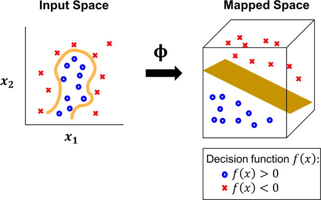
Nonlinear Kernel-induced implicit mapping to higher dimensional space in Support Vector Machine (SVM) modeling

In this study, fault detection is formulated as a supervised learning problem (i.e. classification) with l training instances correspond to batches, where x_i ∊ ℝⁿ. Indices i, j = 1,2,…, l belong to batches, whereas indices k, k′ = 1,2,…, n correspond to input process data features (i.e. process measurements at specific time points). To determine whether an ongoing batch is faulty or normal, we utilize the C-parameterized SVM (C-SVM) classification formulation with nonlinear Kernel functions. The basic C-SVM formulation with hinge loss, ℓ₂-norm penalty, and linear kernel^37,39 is written as:

$$\underset{w,b,\xi }{\text{min}}\frac{1}{2}{\Vert w\Vert }_2^2+C{\displaystyle \sum _{i=1}^l{\mathrm{\xi }}_i}$$

$$\begin{array}{lll}\mathrm{s}.\mathrm{t}.& y_i\left(w\cdot x_i+b\right)\ge 1-{\mathrm{\xi }}_i& i=1,\dots ,l\\ & {\mathrm{\xi }}_i\ge 0& i=1,\dots ,l\end{array}$$ (1)

where w is the weight vector of features (process measurements). ξ_i are slack variables for each instance (i.e. batch) i that are misclassified. C is a regularization parameter and controls the level of training error to be introduced in the cost function for the sake of creating more generalizable models. y_i ∊ {−1,1} denotes the group label of batch i, as normal or faulty, respectively. Finally, b represents the bias parameter. When model 1 is solved to global optimality, resulted optimal solution (w*, b*, ξ*) yields linear decision function (w*, b*, ξ*) whose sign predicts the group membership of the new batch x:

$$w^{\ast }={\displaystyle \sum _{i=1}^l{\mathrm{\alpha }}_i^{\ast }{y}_i{x}_i}$$ (2)

$$f\left(x\right)=w^{\ast }\cdot x+b^{\ast }$$ (3)

where α_i are dual variables. Here, due to the nonlinear nature of batch process data, C-SVM with linear kernel may not provide accurate and robust solutions for batch process monitoring. Therefore, we exploit nonlinear Kernel functions, K(x_i,x_j), within the C-SVM formulation which provides us to train nonlinear decision functions in the input (original) space which implicitly map the data to a different, possibly infinite dimensional feature space where a linear decision function can separate the mapped data⁴⁰. This is also known as Kernel trick (Figure 1). Kernel functions are introduced in the Lagrange dual formulation of model 1, which is written as:

$$\underset{\mathrm{\alpha }}{max}{\displaystyle \sum _{i=1}^l{\mathrm{\alpha }}_i}-\frac{1}{2}{\displaystyle \sum _{i=1}^l{\displaystyle \sum _{j=1}^l{\mathrm{\alpha }}_i}}{\mathrm{\alpha }}_j{y}_i{y}_{j}K\left(x_i,x_j\right)$$

$$\begin{array}{lll}\mathrm{s}.\mathrm{t}.& {\displaystyle \sum _{i=1}^l{\mathrm{\alpha }}_i}{y}_i=0& \\ & {\mathrm{\alpha }}_i\in \left[0,C\right]& i=1,\cdots ,l\end{array}$$ (4)

The resulting linear decision function consisting the optimal dual solution α* becomes:

$$\begin{gathered} f\left(x\right)=w^{\ast }\cdot \varphi \left(x\right)+b^{\ast } \\ ={\displaystyle \sum _{i=1}^l{\mathrm{\alpha }}_i^{\ast }{y}_{i}K\left(x_i,x\right)+b^{\ast }} \end{gathered}$$

where ϕ(x) is the function providing Kernel-induced implicit mapping. Here, w* may no longer belong to ℝⁿ and is possibly of infinite dimension.

The interested reader in the derivation of the Lagrange dual problem and resulting decision functions can refer to the key references^37,39,40.

3 Feature Selection Algorithm based on Nonlinear Support Vector Machines

Here, feature selection algorithm based on nonlinear Support Vector Machines is formulated to attain the most descriptive original process measurements. Elimination of redundant measurements is highly valuable for high-performance model development for batch process monitoring. It significantly reduces probability of over-fitting in the built data-driven models detecting faults, where the size of unfolded and time-evolving batch process data grows significantly. Furthermore, performing dimensionality reduction while protecting the original feature space is highly valuable for rigorous fault diagnosis, where the selected top descriptive features yield the major causes of the detected fault. Below, we present brief theoretical background of the adopted feature selection algorithm which is based on nonlinear Support Vector Machines.

In order to perform model-informed feature selection, we introduce binary variables z ∊ {0,1}ⁿ in the Lagrange dual formulation with nonlinear Kernel functions (model 4), where z_k = 1 corresponds to the selection of feature k as being one of features in the optimal subset and z_k = 0 corresponds to the elimination of feature k. The resulting model becomes:

$$\underset{z}{\text{min}}\underset{\alpha }{max}{\displaystyle \sum _{i=1}^l{\mathrm{\alpha }}_i}-\frac{1}{2}{\displaystyle \sum _{i=1}^l{\displaystyle \sum _{j=1}^l{\mathrm{\alpha }}_i{\mathrm{\alpha }}_j{y}_i{y}_{j}K\left(x_i○z,x_j○z\right)}}$$

$$\begin{array}{lll}\mathrm{s}.\mathrm{t}.& {\displaystyle \sum _{i=1}^l{\mathrm{\alpha }}_i{y}_i}=0& \\ & {\mathrm{\alpha }}_i\in \left[0,C\right]& i=1,\dots ,l\\ & {\displaystyle \sum _k{z}_k}=m& \\ & z_k\in \left\{0,1\right\}& k=1,\dots ,n\end{array}$$ (5)

where m represents the size of the optimally reduced subset of input features and operator ○ is the Hadamard product operator for component-wise multiplication.

Model 5 delineates the explicit formulation of the feature selection problem via nonlinear Support Vector Machines, which results in a challenging bi-level problem. Solving model 5 to global optimality is highly challenging and impractical in real-life applications⁴¹, hence we propose to utilize sensitivity of the inner objective function provided in model 5 with respect to z_k at the optimal solution of the inner maximization problem (α*; z). Here, z_k is treated as a fixed parameter. In order to attain the first-order sensitivity of a model at an optimal solution with respect to a parameter, which is located in the objective function and constraints, we use the partial derivative of the Lagrange function of the model^42–44:

$$\begin{gathered} {\frac{\partial }{\partial z_k}\left[{\displaystyle \sum _{i=1}^l{\mathrm{\alpha }}_i^{\ast }}-\frac{1}{2}{\displaystyle \sum _{i=1}^l{\displaystyle \sum _{j=1}^l{\mathrm{\alpha }}_i^{\ast }}{\mathrm{\alpha }}_j^{\ast }{y}_i{y}_{j}K\left(x_i○z,x_j○z\right)+\lambda \left({\displaystyle \sum _{i=1}^l{\mathrm{\alpha }}_i^{\ast }{y}_i}\right)}-{\displaystyle \sum _{i=1}^l{\mu }_i^{\left(1\right)}{\mathrm{\alpha }}_i^{\ast }}+{\displaystyle \sum _{i=1}^l{\mu }_i^{\left(2\right)}\left({\mathrm{\alpha }}_i^{\ast }-C\right)}\right]|}_{z=z^{\ast }} \\ ={-\frac{1}{2}{\displaystyle \sum _{i=1}^l{\displaystyle \sum _{j=1}^l{\mathrm{\alpha }}_i^{\ast }}{\mathrm{\alpha }}_j^{\ast }{y}_i{y}_j\frac{\partial K\left(x_i○z,x_j○z\right)}{\partial z_k}}|}_{z=z^{\ast }} \end{gathered}$$

where λ ∊ ℝ,μ⁽¹⁾,μ⁽²⁾ ∊ [0, ∞)ⁿ are Lagrange multipliers. Lagrangian sensitivity allows us to guide the perturbations on element z_k. The formulation yields the perturbation criterion for feature k as follows:

$${\text{crit}}_k=={-\frac{1}{2}{\displaystyle \sum _{i=1}^l{\displaystyle \sum _{j=1}^l{\mathrm{\alpha }}_i^{\ast }}{\mathrm{\alpha }}_j^{\ast }{y}_i{y}_j\frac{\partial K\left(x_i○z,x_j○z\right)}{\partial z_k}}|}_{z=z^{\ast }}$$ (6)

$$k_{\text{wrost}}=\arg \underset{k}{\text{max}}{\text{crit}}_k$$ (7)

Using the criterion given in model 6, we eliminate features one at a time (feature worsening the inner objective of model 5 the most, k_worst) as we build nonlinear C-SVM models. This yields a greedy reductive algorithm for model-informed feature ranking. The iterative procedure allows us to perform simultaneous modeling and model-informed feature elimination via C-SVMs. Here, one can also eliminate features in blocks (i.e as % of total features). The presented feature selection algorithm based on nonlinear SVMs is summarized in Figure 2.

Figure 2.

Greedy Reductive Algorithm for Simultaneous Modeling & Model-informed Feature Selection

Of note, the algorithm provided here is equivalent to recursive feature elimination (RFE)-SVM classification algorithm⁴⁵ when performing linear classification. The algorithm has been implemented in C++/Python environment using the LibSVM library⁴⁶. In our previous work, we have successfully applied the presented feature selection algorithm in bioinformatics setting where we achieved profoundly accurate predictions HIV-1 co-receptor usage⁴⁷.

4 Batch Process Benchmark Model & Data Set

The batch process data is adopted from an extensive simulation dataset³⁵ based on penicillin production, PenSim benchmark model³⁸, where the model is expanded with sensor noise (Table 1). The process operates in two modes. It starts in the batch mode with high substrate (glucose) con-centrations that stimulates biomass growth. Then it switches to fed-batch mode with the depletion of glucose where penicillin production is triggered by biomass due to low glucose content in the bioreactor³⁸. pH and temperature of the process is monitored via closed-loop PID controllers, where aeration rate, agitator power, feed rate, feed temperature, hot and cold water temperatures are in open loop. Schematic diagram of the fed-batch penicillin production is given in Figure 3.

Table 1.

List of Online Measurements

Online Measured Variables		Measurement Noise (σ)
1.	Fermentation volume [m3]	0.002
2.	Dissolved O2 concentration [mg/L]	0.004
3.	Dissolved CO2 concentration [mg/L]	0.12
4.	Reactor temperature [K]	0.1
5.	pH[−]	0.02
6.	Feed rate [L/h]	1%
7.	Feed temperature [K]	0.1
8.	Agitator power [W]	1%
9.	Cooling/heating medium flow rate [L/h]	1%
10.	Heating medium temperature [K]	0.1
11.	Hot/cold switch [−]	–
12.	Base flow rate [mL/h]	1%
13.	Acid flow rate [mL/h]	1%

Figure 3.

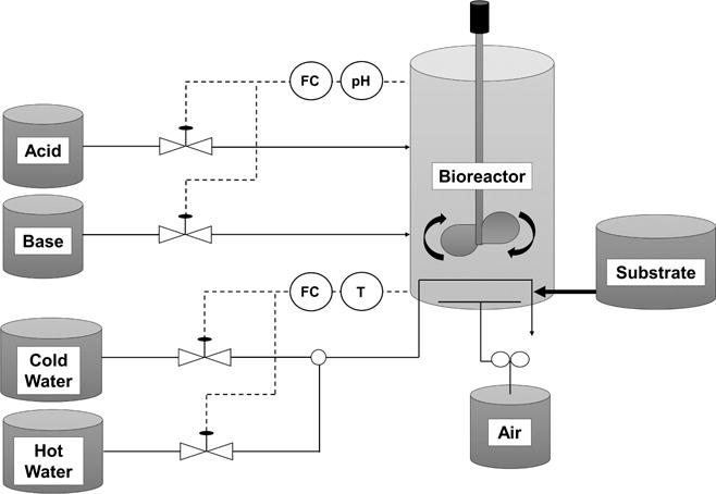
Fed-batch Penicillin Production Flow Diagram

In this paper, we use the aligned, base case simulation data introduced in Van Impe et. al where the initial fermenter volume, biomass concentration, and substrate concentration are independently sampled from normal distributions providing batch-to-batch variability³⁵. The alignment is done by bringing all simulated batches to equal length via indicator variables as described in Birol et. al³⁸. The data set includes 400 normal and between 1000-2000 batches per 15 different simulated process faults yielding 22,200 faulty batches in total. Table 2 tabulates 15 different fault types and corresponding number of batches simulated for each of them.

Table 2.

Overview of Faults & Corresponding No of Batches in the Data Set

Fault		No of Batches
1.	Sudden change in feed substrate concentration	2000
2.	Change in coolant temperature	2000
3.	Agitator power drop	1600
4.	Aearation rate drop	1600
5.	Gradual change of feed rate	1200
6.	Gradual dissolved oxygen sensor drift	2000
7.	Feed temperature change	1600
8.	pH sensor drift	1600
9.	Non-functional pH control	1200
10.	Reduced pH control	1200
11.	Reactor temperature sensor bias	1200
12.	Reactor temperature sensor drift	1600
13.	Reduced temperature control	1200
14.	Reduced temperature control - maximal flow not impacted	1200
15.	Contamination	1000

We have considered 13 process variables (5 state and 8 manipulated) that can be measured online (Table 1). In this work, we use cumulative acid/base flows [mL] instead of instantaneous flow rates as they are suggested to be relatively more informative³⁵. Each batch is completed in about 460 h where the sensors are sampled in every 0.02 h. When aligned, this corresponds to a total batch length of 1201 samples which results in 3-dimensional (3D) batch process dataset of size 1400-2400 batch × 13 variable × 1201 sample (time point).

5 Proposed Framework for Simultaneous Fault Detection & Diagnosis in Batch Processes

The proposed framework consists of two phases: (i) Offline phase includes the formulation of the fault and time-specific models for fault detection and diagnosis via historical signal process data where the novel optimization-backed feature selection algorithm is used; (ii) Online phase monitors ongoing batches in real-time by using the fault and time-specific models. Prior to both phases, data needs to be re-organized and/or processed.

5.1 Data Preprocessing

Here, we (i) divide the time horizon into intervals of fixed size which we refer as sample bins, (ii) unfold 3-dimensional batch process data into 2-dimension via batch-wise unfolding⁴⁸, (iii) incorporate additional informative features (feature extraction) from sample bins, (iv) normalize the obtained 2-dimensional data, and (v) eliminate the features having less than 10⁻⁸ standard deviation, respectively.

Step-1: Creating Sample Bins

Batch process data is 3 dimensional. For each batch at each specific time point, it includes a process variable measurement. This initial step of data preprocessing slightly differs for offline and online phase.

In the offline phase, the motivation is to produce an online fault detection & diagnosis decision support tool for end-users, therefore we need to develop time-specific models for each fault. To do this, first, we partition the time horizon into intervals of fixed size and group the process variable measurements of batches at particular time periods. We refer these time periods as sample bins. Next, we train models for fault detection and diagnosis for each sample bin to obtain time-specific models. Here, the size of sample bins is a user-defined parameter. Selection of smaller bin size implicitly increases the number of checks on an ongoing batch, thus accelerates the detection of possible fault occurrences, yet increasing the number of models to be developed. In this study, we have selected the sample bin size as 10 which has resulted in total of 120 sample bins spanning the entire time horizon.

In the online phase, data is continuously collected. In order to analyze the incoming 3-dimensional data with the developed time-specific models, we need to gather the batch process measurements from the relevant time points and form the sample bins for further analysis.

Step-2: Unfolding 3D Batch Process Data into 2D

In order to train models with 3-dimensional batch process data, we need to unfold it into a 2-dimensional matrix via one of the three possible ways: (i) batches, (ii) process variable measurements, or (iii) time points. In this paper, we adopt batch-wise unfolding approach⁴⁸. The batch-wise data unfolding yields batches as the incidents (rows), and process variables at specific time points as the features (columns) of the 2-dimensional dataset. Of note, while we are unfolding the 3-dimensional data in each sample bin, we solely include the relevant (observed) process variable measurements. This data re-configuration enables inspection of batches in regular periods via time-specific models that use historical and most recent process signal data to determine whether the batch is performing well or not while the batch is still ongoing. The illustration of data structure preprocessing, that involves Step 1 and 2, is shown in Figure 4.

Figure 4.

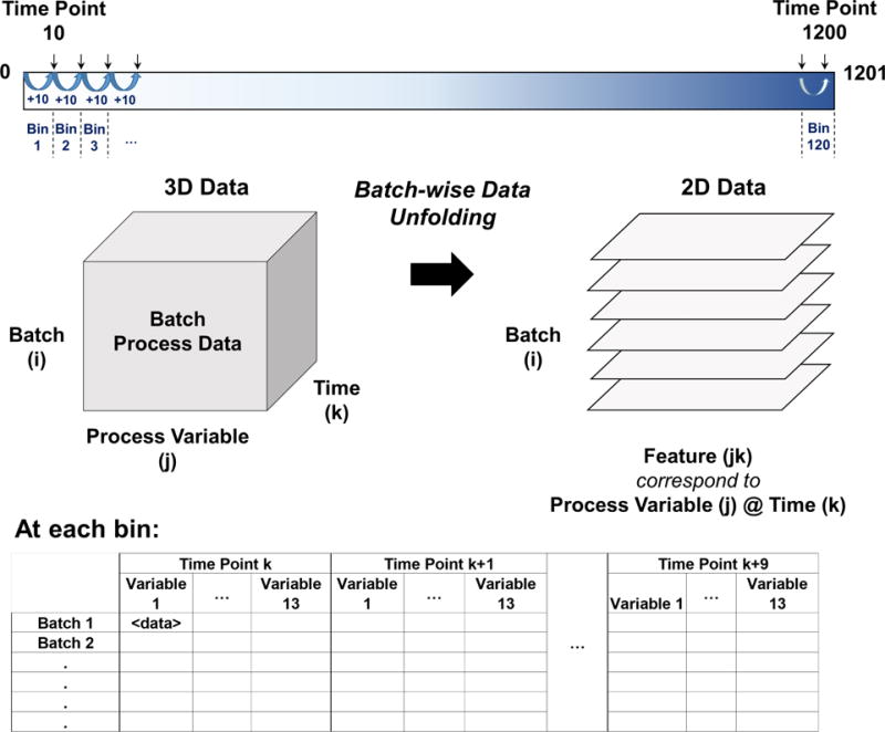
Data Preprocessing: Unfolding the Batch Process Data and Formation of Sample Bins

Step-3: Extracting Additional Features

In order to improve the data-driven modeling accuracy, we extract and incorporate additional features that can characterize process behavior of each batch at each sample bin. In this study, in addition to the historical and most recent process variable measurements, we have utilized slope, standard deviation, and mean of 13 process variables (referred as process behavior features) within each sample bin. The case-specific addition of the features is given in Section 6. Here, we would like to highlight that the end-users of the presented framework will be allowed to include/exclude any type of process behavior features during the model development phase. In case of highly noisy plant data, one can always smoothen the data by using filters (i.e Kalman filter), and extract features from the filtered data to further use in the model building phase.

Step-4&5: Data Normalization & Reduction

Finally, we normalize the re-configured and extended 2-dimensional matrix within each sample bin and perform a priori dimension reduction by eliminating the features (process variable measurements at specific time points and extracted features describing process behavior) with less than 10⁻⁸ standard deviation.

5.2 Offline Phase: Model Building

In offline phase, we build fault and time-specific nonlinear Support Vector Machine classification models by using historical and/or simulation-based batch process signal data. Particularly, we train and test 15 separate C-SVM classification models per sample bin for detection and diagnosis of 15 distinct faults. To do this, we (i) select the preprocessed data of faulty and normal batches that have been observed within the selected time period (i.e. sample bin), (ii) create balanced training and test sets with 20 runs of 5-fold cross-validation, (iii) tune the hyperparameters C and γ of the (C-SVM) classification models, (iv) perform simultaneous feature selection and model building via nonlinear Support Vector Machines, (v) build C-SVM classification models with average feature rank list, and (vi) test model accuracies to determine the end-model to be implemented in the online phase, respectively.

Step-1: Collecting Preprocessed Batch Process Data

In the first step of the offline model building, we retrieve the preprocessed 2-dimensional process data of faulty and normal batches that have been observed within the time period of the selected sample bin (Figure 5).

Figure 5.

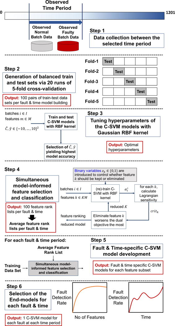
Offline Phase of the Proposed Simultaneous Fault Detection & Diagnosis Framework

Step-2: Generating Train and Test Data Sets

In order to have accurate and robust models, we need to balance the number of batches that belong to different class labels. In other words, we need to have equal amount of faulty and normal batches in training and test sets. Therefore, the next step in offline model building phase is to determine the number of faulty and normal batches within the observed sample bin period separately, include the limiting number of batches of one class label, and randomly select the same number of batches from the pool of batches with the other class label that have been observed within the specified time period. Then, we perform 5-fold cross-validation with 20 runs to create training-testing datasets in order to minimize generalization error and avoid over-fitting. This results in 100 training-testing dataset pair generation.

Step-3: Tuning Hyperparameters for C-SVM Models

Next, we tune the hyperparameters C and γ of the C-SVM (two-class) classification models by using Gaussian radial basis function (RBF),

$$K\left(x_i,x_j\right)=\exp \left(-\mathrm{\gamma }{\Vert x_i-x_j\Vert }^2\right),$$ (8)

as the nonlinear Kernel function. The appropriate selection of hyperparameters is necessary for the sake of generalization error minimization. The density of the data is a critical factor in the selection of hyperparameter γ to avoid over-fitting in the resulted separating decision function model. The default value for RBF kernel hyperparameter, γ, used by LIBSVM is 1/n, where n is the number of features. Therefore, we tune parameter $\widehat{\mathrm{\gamma }}$ where

$$\mathrm{\gamma }=\frac{2^{\widehat{\mathrm{\gamma }}}}{n}.$$ (9)

Similarly, we tune parameter $\widehat{C}$, where the relation between $\widehat{C}$ and C is:

$$C=2^{\widehat{C}}.$$ (10)

According to the described iterative feature selection algorithm in Section 3, $\widehat{\mathrm{\gamma }}$ can be updated in each iteration with the available set of features:

$$\mathrm{\gamma }=\frac{2^{\widehat{\mathrm{\gamma }}}}{z^{\mathbf{\top }}\mathbf{1}}$$ (11)

In this work, tuning is performed for parameters $\widehat{C}$, and $\widehat{\mathrm{\gamma }}$ via a grid search for all value combinations between −10: 10. We train and test models using all features of 100 training-testing dataset pairs with every combination of $\widehat{C}$ and $\widehat{\mathrm{\gamma }}$ parameters. Here, instead of repeating grid search for hyperparameters tuning after each iteration of feature elimination, which would be ideal but inefficient, we perform tuning at first iteration where we include the whole set of features. Then, the hyperparameters with the highest average testing accuracy are chosen for the next steps.

Step-4: Simultaneous Model-informed Feature Selection and Classification

The tuned hyperparameters are incorporated into simultaneous model-informed feature selection and classification algorithm via C-SVMs which is described in Section 3. Here, we iteratively build C-SVM binary classification models with Gaussian radial basis function (RBF) kernel starting from the complete set of features until we are left with the last feature in the data set. In each iteration, we eliminate features based on the Lagrangian sensitivity of the dual objective function of the built C-SVM model (specifically, the inner objective function of Model 5) with respect to the feature subset size. This iterative procedure is performed with each of the 100 training and testing data set pairs which creates 100 feature rankings for each fault class at each sample bin. Subsequently, one average feature ranking list is created for each fault and sample bin combination according to the statistical distribution of the feature ranks across 100 individual ranking lists.

Step-5: Building C-SVM Models with Average Feature Rank Lists

At this stage, we train C-SVM classification models with Gaussian RBF kernel with the same 100 training and testing data set pairs by using the fault and time-specific average feature ranking lists. Starting from the entire feature set and eliminating one feature at a time according to the average fault and time specific feature rank list, we train 100 C-SVM classification models for each feature subset. The model performances are then evaluated via several metrics, and averaged for each feature subset. These metrics are fault detection rate (recall), accuracy, area under the receiver operator curve (AUC), and false alarm rate. Thus, we obtain one fault and time-specific C-SVM model per each feature subset.

Step-6: Choosing the End-models for Online Phase

In the last stage of the offline phase, we determine the end-models (fault and time-specific C-SVM models). Among the all developed fault and time-specific C-SVM models for each feature subset, the ones yielding the highest fault detection rate are selected. These are referred as the end-models. The end-models, that have the optimal feature subset for maximum fault detection rate, are aimed to be further implemented in the online phase. The overall framework of offline phase is summarized in Figure 5.

5.3 Online Phase: Fault Detection & Diagnosis

In this phase, we implement the fault and time specific end-models to create a decision support tool for online fault detection & diagnosis. These are selected binary classifiers, the optimal decision functions, which will evaluate the incoming preprocessed online batch process data and produce a binary answer for fault occurrence. The fault and time-specific classifier models inherently include the optimal set of features, which are the most informative process measurements/characteristics, to diagnose the detected fault at the time period of interest. Therefore, the end-models are able to provide instantaneous rank-ordered root-cause analysis when a fault occurs, which enables them to be employed as an online simultaneous fault detection & diagnosis tool. The end-user can further interpret and link the rank-ordered fault diagnosis to corrective actions to reverse the fault. The schematic representation of the implementation of the models for online phase is shown in Figure 6.

Figure 6.

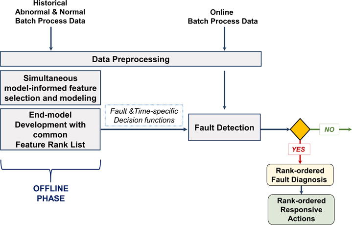
Online Phase Implementation for Simultaneous Fault Detection & Diagnosis

6 Case Studies

We have performed three sets of experiments to test the performance of the proposed data-driven framework: (i) one-step rolling time horizon analysis, where fault detection and diagnosis models are built for each individual sample bin; (ii) two-step rolling time horizon analysis, in which models are developed for every two sliding sample bins; and (iii) evolving time analysis, where we build models by using data within the selected sample bin and set of informative features from all previous sample bins. Below we describe each of the analysis, and provide corresponding results. The performance of the developed models is assessed via (i) fault detection rate (also known as true positive rate or recall), (ii) accuracy, (iii) false alarm rate, and (iv) Area Under the Receiver Operating Characteristic (ROC) Curve, (AUC). The ideal models would have perfect Area Under the ROC curve, accuracy, as well as fault detection rate being 1 with minimum False Alarm Rate (ideally, 0). The results of all fault & time-specific models with each time horizon approach is provided in the Supplementary material.

6.1 Fault Detection & Diagnosis with One-Step Rolling Time Horizon Approach

Here, we inspect the status of a given batch with a total of 1800 fault and time-specific end-models, for 15 different faults (Table 2) at each of the 120 sample bins. We only consider the process data within each selected sample bin time period, and exclude any information from previous sample bins. Since, batch monitoring is performed within each sample bin individually, we refer this approach as one-step rolling time horizon approach.

Initial step in the one-step rolling time horizon approach is to gather the preprocessed data sets relevant to each sample bin. Here, the features of the data sets include the process variable measurements as well as slope, standard deviation and mean of each 13 process variables within each sample bin of size 10. This results in 169 features per bin, where 130 of them belong to actual measurements and 39 characterizes the process behavior. On the other hand, the number of instances, which is the number of normal and faulty batches, varies along the time horizon. In each sample bin, we include only the normal and faulty batch data that have been observed between the time period of the selected sample bin. In particular, we have 400 normal and 1000-2000 faulty batches per fault (Table 2). When building models with one-step rolling time horizon approach, we select the faulty batches among the batches where the fault has already been introduced before the initial time point of the selected sample bin. Then, as mentioned in Section 5.2, we form balanced training and testing datasets including equal amount of normal and faulty batches for each model development. We have less faulty batches in the beginning of the process operation, therefore the dataset used to train a model for an early time period is smaller compared to later. In other words, the data set size changes as we move along the time horizon due to the change in the number of batches with varying fault onset time.

We have demonstrated 3 faults with varying level of difficulty in detection at the selected sample bins to evaluate the performance of the one-step rolling time horizon approach (Table 3). Fault 7 (change in feed temperature) is reported to be the easiest fault to detect due to the presence of feed temperature measurements in the batch process data set. Fault 8 (pH sensor drift) poses moderate difficulty to be detected, whereas Fault 15 (contamination) is defined as one of the most challenging faults of the adopted dataset³⁵. The complete set of fault and time-specific model results can be found in the Supplementary. Table 3 reports the selected fault and time specific models (end-models) with their corresponding optimal feature subset size, fault detection rate, model accuracy, AUC, and false alarm rate. When a fault is detected with these models, the corresponding optimal feature subset reveals the explicit process measurements (and/or features describing process behavior) for diagnosis of the detected fault. For particular models, that are marked with asterisks, we have provided a second alternative model, where we are able to attain almost equivalent fault detection rate with significantly lower optimal feature subset size (Table 3). This consequently facilitates the isolation and correction of the detected fault by enabling optimal sensor placement (i.e. sensor network design). Furthermore, obtaining the maximum model performance with minimum number of features is favorable in terms of computational efficiency and simplicity. Figure 7 shows an example for such cases through Fault 8 at Sample Bin 12.

Table 3.

One-step Rolling Time Horizon Analysis: Selected Model Performances for Fault 7 (easy), 8 (moderate), and 15 (challenging)

Fault	Sample Bin	Fault Detection Rate	Optimal Feature Subset Size	Accuracy	False Alarm Rate	AUC
Fault-7 Feed Temperature Change	20	0.98	1	0.99	0.00	1.00
	40	0.98	1	0.99	0.00	0.99
	60	1.00	3	1.00	0.00	1.00
	80	1.00	3	1.00	0.00	1.00
	100*	1.00	3	1.00	0.00	1.00
	100	1.00	1	1.00	0.00	1.00
	120*	1.00	9	1.00	0.00	1.00
	120	1.00	1	1.00	0.00	1.00
Fault-8 pH Sensor Drift	20	0.70	16	0.77	0.15	0.84
	40*	0.94	9	0.97	0.00	0.99
	40	0.94	2	0.97	0.00	0.99
	60*	0.96	4	0.98	0.00	1.00
	60	0.96	2	0.98	0.00	1.00
	80*	0.95	34	0.97	0.00	0.99
	80	0.95	2	0.97	0.00	0.99
	100*	0.96	27	0.98	0.00	1.00
	100	0.96	25	0.98	0.00	1.00
	120*	0.97	28	0.98	0.00	1.00
	120	0.97	6	0.98	0.00	1.00
Fault-15 Contamination	20	0.74	99	0.61	0.53	0.65
	40*	0.81	31	0.88	0.04	0.94
	40	0.81	28	0.88	0.04	0.94
	60*	0.97	43	0.98	0.01	0.99
	60	0.97	29	0.98	0.01	0.99
	80*	0.98	68	0.99	0.00	1.00
	80	0.98	10	0.99	0.00	1.00
	100*	0.98	56	0.99	0.00	1.00
	100	0.98	35	0.99	0.00	1.00
	120*	1.00	10	1.00	0.00	1.00
	120	1.00	8	1.00	0.00	1.00

Figure 7.

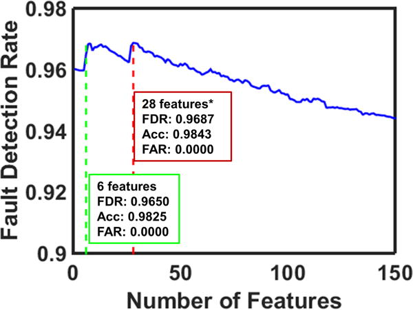
Selecting the Optimal Feature Subset for Detection & Diagnosis of Fault 8 at Sample Bin 120. (FDR: Fault Detection Rate, Acc: Accuracy, FAR: False Alarm Rate)

The models built via one-step rolling time horizon approach reveals perfect detection rate, and accuracy for Fault 7 with zero false alarm rate and small optimal feature subset size. As the detection difficulty increases (from Fault 7 to Fault 15), we observe that the early time-specific models (prior to Sample bin 20) have shown relatively high false alarm rates. This may stem from the relatively low number of faulty batches in the early periods of the process simulation, and can be overcome by simulating additional batches with earlier fault onset time. On the other hand, the performance of the models of the later sample bins improve with the inclusion of more batch data. False alarm rates immediately become ideal by approaching to 0 later in the batch process regardless of the difficulty level of the fault detection.

Another observation is that the increase in the fault complexity is reflected with an increase in the average feature subset size across the all time-specific models of each fault.

Figure 8 depicts the fault detection rate of all fault and time-specific models built for each feature subset. Among them, the end-model is the one yielding the highest fault detection rate, highlighted with a red line, where corresponding feature subset size, model accuracy and false alarm rate are reported. As mentioned before, the results with asterisks imply the existence of an alternative model with almost equivalent fault detection rate with considerably lower feature subset size, which are listed in Table 3.

Figure 8.

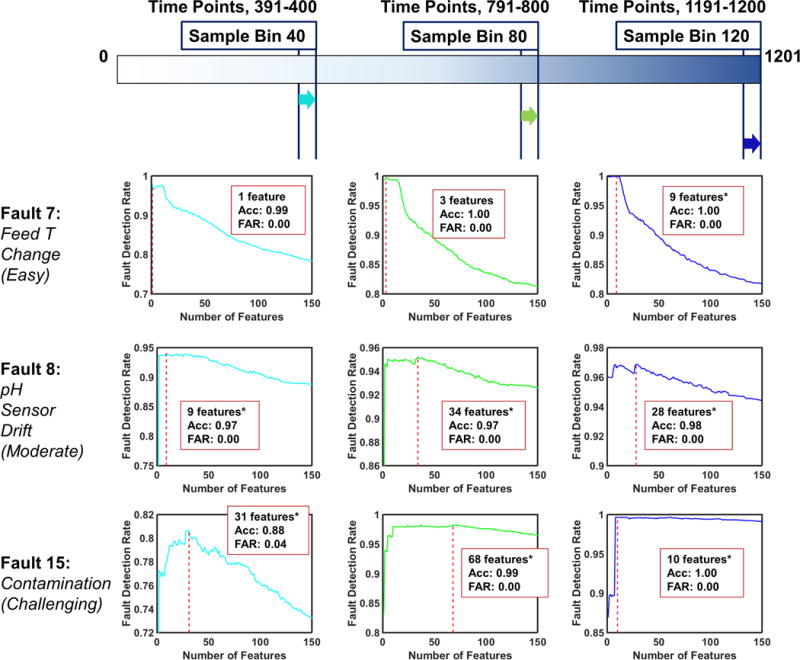
One-step Rolling Time Horizon Analysis: Detection Rates of 3 faults with increasing level of difficulty in detection; Fault 7,8, and 15 respectively. The optimal number of features, detection accuracy and false alarm rate are provided at the highest detection rate. The results with asterisks indicate the existence of an alternative model producing almost equivalent performance with less features. Alternative models are provided in Table 3.

6.2 Fault Detection & Diagnosis with Multi-Step Rolling Time Horizon Approach

In this approach, we monitor a given batch with a total of 1785 fault and time-specific end-models throughout the process. The models examine for 15 separate faults at every two successive sample bins in a sliding manner which corresponds to 119 checks. In addition to the process variable measurements of the later sample bin, we consider set of features from the former sample bin that characterize process behavior. In this case, we have exploited data of one previous sample bin in addition to the selected sample bin for each time-specific model development. This has enabled us to analyze the 3-dimensional batch process data via two-step rolling time horizon approach. Particularly, this approach can be extended with addition of further previous sample bins, therefore we call it as multi-step rolling time horizon approach.

In this case, similar to one-step rolling time horizon approach, initial step is to arrange two-step sample bins and collect the preprocessed data sets. We have two-fold feature subsets in this approach, one set identifying the former sample bin, and later defining the recent process progress. The former feature subset contains solely the process behavior characterizing features; slope, standard deviation and mean of 13 process variable measurements within that previous sample bin, resulting in 39 features. The later feature subset consists of the process measurements as well as slope, standard deviation and mean of each 13 process variables within the latest sample bin, resulting in an additional 169 features per bin. As a result, we incorporate 208 features in each time-specific model development with two-step rolling time horizon approach. Here, similar to the one-step rolling time horizon approach, the number of batches involved during model development changes according to time due to the variation in fault onset time.

Table 4 tabulates the selected fault and time specific models (end-models) with the corresponding performance. Similarly, the alternative model results are listed in Table 4.

Table 4.

Two-step Rolling Time Horizon Analysis: Selected Model Performances for Fault 7 (easy), 8 (moderate), and 15 (challenging)

Fault	Sample Bin	Fault Detection Rate	Optimal Feature Subset Size	Accuracy	False Alarm Rate	AUC
Fault-7 Feed Temperature Change	19–20*	0.83	21	0.92	0.00	1.00
	19-20	0.83	10	0.91	0.00	1.00
	39-40	1.00	1	1.00	0.00	1.00
	59-60	1.00	1	1.00	0.00	1.00
	79–80*	1.00	2	1.00	0.00	1.00
	79-80	1.00	1	1.00	0.00	1.00
	99–100*	1.00	6	1.00	0.00	1.00
	99-100	1.00	1	1.00	0.00	1.00
	119-120	0.75	1	0.88	0.00	1.00
Fault-8 pH Sensor Drift	19–20*	0.83	52	0.85	0.13	0.93
	19-20	0.83	49	0.85	0.12	0.93
	39-40	0.98	4	0.99	0.00	1.00
	59–60*	0.97	3	0.99	0.00	1.00
	59-60	0.97	2	0.98	0.00	1.00
	79–80*	0.98	32	0.99	0.00	1.00
	79-80	0.98	9	0.99	0.00	1.00
	99–100*	0.98	66	0.99	0.00	1.00
	99-100	0.98	3	0.99	0.00	1.00
	119–120*	0.99	70	1.00	0.00	1.00
	119-120	0.99	1	0.99	0.00	1.00
Fault-15 Contamination	19–20*	0.57	204	0.58	0.41	0.61
	19-20	0.57	201	0.58	0.41	0.61
	39-40	0.94	58	0.96	0.02	0.99
	59–60*	0.99	57	1.00	0.00	1.00
	59-60	0.99	18	0.99	0.01	1.00
	79–80*	0.99	72	1.00	0.00	1.00
	79-80	0.99	42	0.99	0.00	1.00
	99–100*	1.00	77	1.00	0.00	1.00
	99-100	1.00	5	1.00	0.00	1.00
	119–120*	1.00	145	1.00	0.00	1.00
	119-120	1.00	8	1.00	0.00	1.00

Similar to the previous approach, we observe that fault detection rates improve with time for all faults, and the optimal feature subset size increases as the faults become more challenging to detect. Finally, we notice a significant improvement in the fault detection rate of Fault 15 time-specific models after Sample Bins 18-20 compared to the models obtained via one-step rolling time horizon approach, which indicates that the added features have helped models to gain more insight to detect this challenging fault.

Figure 9 demonstrates the fault detection rate of the entire fault and time specific models built for each feature subset. The end-models are shown with red-dashed lines.

Figure 9.

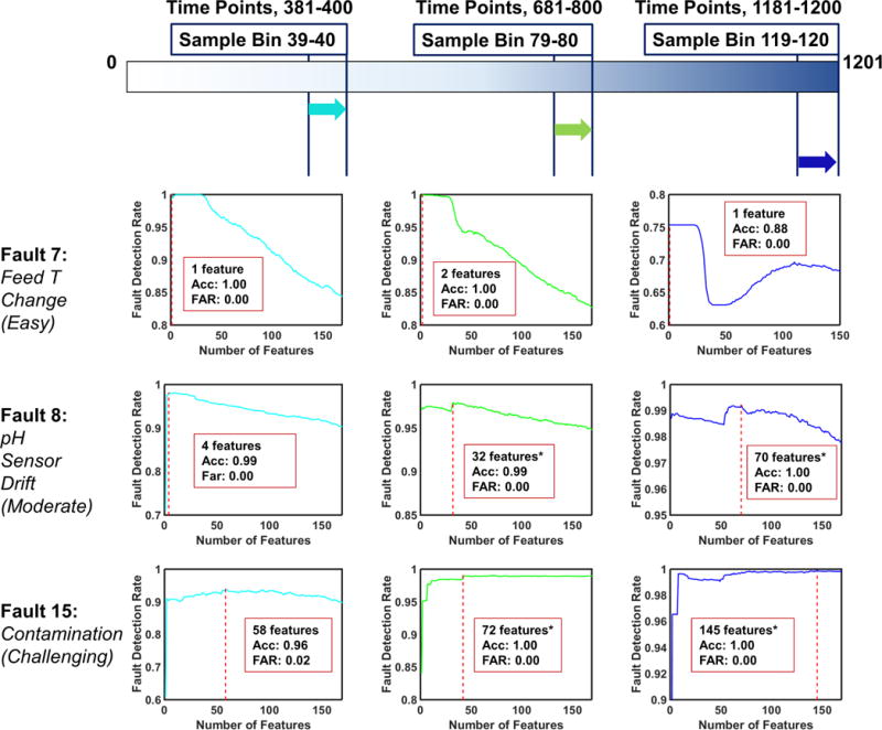
Two-step Rolling Time Horizon Analysis: Detection Rates of Fault 7,8, and 15. The optimal number of features, detection accuracy and false alarm rate are provided at the highest detection rate. The results with asterisks indicate the existence of an alternative model producing almost equivalent performance with less features. Alternative models are provided in Table 4.

6.3 Fault Detection & Diagnosis with Evolving Time Horizon Approach

As a third and final case study, we adopt evolving time horizon approach, where we build models by making use of the entire historical process data until the last time point of the selected sample bin for analysis. Here, we monitor a given batch with a total of 1800 fault and time-specific end-models where the given batch is scanned for 15 different faults (Table 2) at each of the 120 sample bins. We train models by exploiting the entire historical batch process data at each sample bin, therefore we refer this approach as evolving time horizon approach.

This approach is equivalent to the multi-step rolling time horizon approach, when one incorporates the process behavior features from the entire previous sample bins, instead of only one. This corresponds to the collection of slope, standard deviation and mean of 13 process variable measurements from all previous and the most recent sample bins as well as the actual process measurements observed within the latest sample bin. Consequently, the data set size grows significantly as we move along the time horizon, where the number of features range between ~ 170–4400.

Table 5 exhibits the chosen fault and time specific models for the online phase (end-models) obtained via evolving time horizon based analysis. Compared to the other time horizon approaches, the fault detection rates attained with this approach for Fault 8 and 15 either remain same or slightly improve. On the other hand, the model performances for Fault 7 time-specific models significantly deteriorate. This may be an indicator of the increased noise level in the data. In other words, aggregation of the entire historic process data has possibly elevated the amount of redundant features, consequently deteriorated the performance of the models for Fault 7 (the easiest fault to detect). Another remarkable observation is the significant increase in the optimal feature subset sizes for Fault 7 and 15, which makes the evolving time horizon approach not preferable compared to the other two approaches.

Table 5.

Evolving Time Horizon Analysis: Selected Model Performances for Fault 7 (easy), 8 (moderate), and 15 (challenging)

Fault	Sample Bin	Fault Detection Rate	Optimal Feature Subset Size	Accuracy	False Alarm Rate	AUC
Fault-7 Feed Temperature Change	20	0.80	143	0.89	0.02	0.97
	40*	0.81	407	0.88	0.05	0.95
	40	0.81	406	0.88	0.04	0.95
	60*	0.77	348	0.87	0.02	0.95
	60	0.77	320	0.87	0.03	0.95
	80*	0.79	401	0.88	0.04	0.95
	80	0.79	233	0.88	0.03	0.94
	100	0.80	721	0.87	0.06	0.94
	120*	0.83	433	0.90	0.03	0.96
	120	0.83	427	0.89	0.04	0.96
Fault-8 pH Sensor Drift	20	0.79	93	0.83	0.12	0.91
	40*	0.90	20	0.95	0.00	0.99
	40	0.90	12	0.95	0.00	0.99
	60*	0.96	89	0.98	0.00	1.00
	60	0.96	82	0.98	0.00	1.00
	80*	0.97	87	0.99	0.00	1.00
	80	0.97	4	0.98	0.00	0.99
	100*	0.98	13	0.99	0.00	0.99
	100	0.98	7	0.99	0.00	0.99
	120*	1.00	17	1.00	0.00	1.00
	120	1.00	5	1.00	0.00	1.00
Fault-15 Contamination	20	0.66	1	0.50	1.00	1.00
	40*	0.92	226	0.95	0.02	0.99
	40	0.92	172	0.95	0.02	0.99
	60*	0.99	523	0.99	0.00	1.00
	60	0.99	268	0.99	0.00	1.00
	80*	0.99	496	1.00	0.00	1.00
	80	0.99	323	0.99	0.00	1.00
	100*	0.99	684	0.99	0.00	1.00
	100	0.99	84	0.99	0.00	1.00
	120*	1.00	193	1.00	0.00	1.00
	120	1.00	55	1.00	0.00	1.00

Figure 10 shows the fault detection rate of all fault and time specific models built for each feature subset. The end-models are highlighted with red dashed lines.

Figure 10.

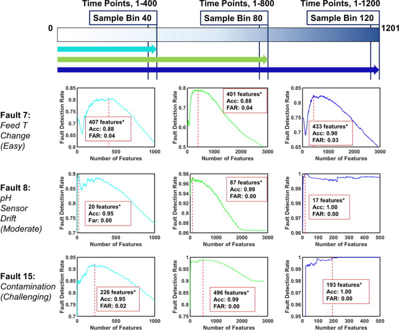
Evolving Time Horizon Analysis: Detection Rates of Fault 7,8, and 15. The optimal number of features, detection accuracy and false alarm rate are provided at the highest detection rate. The results with asterisks indicate the existence of an alternative model producing almost equivalent performance with less features. Alternative models are provided in Table 5.

6.4 Comparison

Here, we compare the performance of the fault and time-specific models built via three distinct time horizon approaches through Fault 7,8, and 15 (three faults with varying level of difficulty to detect). Figure 11 depicts the variation of fault detection rate with respect to time (i.e. sample bin) for one-step rolling, two-step rolling, and evolving time horizon approaches. The fault detection rate versus time plots for all faults are provided in Figure A1.

Figure 11.

Comparison of the Fault Detection Rates for Fault 7,8, and 15 along the Batch Process with respect to One-step Rolling, Two-step Rolling, and Evolving Time Horizon approaches

As one can notice, performance of different time horizon approaches are not consistent across the all faults; they are fault-specific. However, it is evident that as the detection difficulty level increases, two-step rolling and evolving time horizon analysis performs better than the other approach, which prevails the increasing significance of historical data usage for more challenging faults.

One major observation is the relatively low fault detection rate and accuracy in early time models among all time horizon approaches. This is mainly due to the faulty batch data scarcity in early time models (until sample bin 30), which implies low number of simulated batches with fault in early periods of the process due to varying fault onset times. Such scarcity affects the number of batches included during the model development in the offline phase. In early time models, the number of faulty batches is limiting case. However, the situation is reversed as we move along the time horizon. The number of simulated batches, in which fault has been introduced by then, exceed the number of simulated batches under normal conditions. In order to be consistent during model development and learn both class equally, we equate the number of normal and faulty batches before we train our fault detection and diagnosis models. This leads us to use of datasets with varying sizes along the process for different time-specific models. The size of the adopted dataset changes in two ways: (i) number of batches involved, and (ii) number of extracted features. The afore-mentioned fluctuation in the number of simulated faulty batches along the simulation alters the dataset dimension by changing the number of batches involved. On the other hand, the number of features changes with the adopted time horizon approach. Particularly, the smallest dataset used for model development belongs to the first sample bin of one-step rolling time horizon analysis (Sample Bin 2), where we train our fault-specific models with 12 faulty and 400 normal batches, and 142 features (after eliminating the ones with less than 10⁻⁸ standard deviation among 169 features). Whereas the largest data set is observed at the final sample bin of the evolving time horizon approach, where we have 2000 faulty and 400 normal batches, and 4381 features (after the aforementioned elimination based on the standard deviation threshold).

Another possible reason for relatively lower performance of the models in early time of the process is the change in the operation mode. The process begins in a batch mode and switches to fed-batch mode once the substrate (i.e. glucose) concentration is nearly depleted. Since we have no flows into the bioreactor, thus no information of feed flow rate in batch mode as we do in fed-batch mode, the number of features contributing model development during that period decreases. This may have also caused the decrease in model performance in early time of the process.

During the detection of a moderate fault, Fault 8, we observe that all three time horizon approaches perform similar in early time models, where two-step rolling time horizon technique becomes superior in later stages. Whereas for the detection of a challenging fault, Fault 15, evolving time horizon approach competes with two-step rolling time horizon, and indeed dominates it in early time models in terms of the fault detection rate. Yet, for the sake of computational efficiency and simplicity, selection of the end-models via two-step rolling time horizon approach would be favorable over the end-models assessed by the evolving time horizon approach. Regardless of the fault and the time horizon approach, fault detection rates of early time models need to be improved and this can be achieved with further set of simulations where faults can be introduced earlier.

Finally, we present a comparative analysis for fault diagnosis through Fault 8. The diagnosis is provided for the Sample Bin 40, 80, and 120 models formed via one-step rolling (12), two-step rolling (13), and evolving (14) time horizon approaches. The color codes represent the Sample Bin index in Figures 8, 9, and 10, where cyan, green and blue represents Sample Bin 40, 80, and 120 models, respectively. Of note, for the cases where we have superior alternative models, we have adopted their optimal feature subset for fault diagnosis. The explicit list of features (process measurements and/or process behavior describing features) for fault diagnosis with the three time horizon approaches are given in Tables 6, 7, and 8, respectively.

Table 6.

Diagnosis of Fault 8 at Sample Bin 40 via One-step Rolling, Two-step Rolling, and Evolving Time Horizon based Analysis. (HPV: historic process variable, HPB: historic process behavior, CPV: current process variable)

Approach	Sample Bin 40
	Feature Rank	Feature Type	Corresponding Time Point	Feature Name
One-step Rolling Time Horizon	1	HPB	391-400	Slope of Cumulative Acid Flow Rate
	2	HPB	391-400	Standard deviation in Cumulative Acid Flow Rate
Two-step Rolling Time Horizon	1	HPB	381-390	Slope of Cumulative Acid Flow Rate
	2	HPB	381-390	Standard deviation in Cumulative Acid Flow Rate
	3	HPB	381-390	Mean of Cumulative Acid Flow Rate
	4	CPV	400	Dissolved CO2 Concentration
Evolving Time Horizon	1	HPB	51-60	Mean of pH
	2	HPB	31-40	Mean of pH
	3	HPB	61-70	Mean of pH
	4	HPB	71-80	Slope of Cumulative Acid Flow Rate
	5	HPB	71-80	Standard deviation in Cumulative Acid Flow Rate
	6	HPB	141-150	Mean of Cumulative Acid Flow Rate
	7	HPB	151-160	Mean of Cumulative Acid Flow Rate
	8	HPB	81-90	Slope of Cumulative Acid Flow Rate
	9	HPB	161-170	Mean of Cumulative Acid Flow Rate
	10	HPB	171-180	Mean of Cumulative Acid Flow Rate
	11	HPB	131-140	Mean of Cumulative Acid Flow Rate
	12	HPB	61-70	Slope of Cumulative Acid Flow Rate

Table 7.

Diagnosis of Fault 8 at Sample Bin 80 via One-step Rolling, Two-step Rolling, and Evolving Time Horizon based Analysis. (HPV: historic process variable, HPB: historic process behavior, CPV: current process variable)

Approach	Sample Bin 80
	Feature Rank	Feature Type	Corresponding Time Point	Feature Name
One-step Rolling Time Horizon	1	HPB	791-800	Mean of pH
	2	HPV	794	Hot/cold Switch
Two-step Rolling Time Horizon	1	HPB	781-790	Mean of pH
	2	HPB	791-800	Mean of pH
	3	HPV	787	Hot/cold Switch
	4	HPV	787	Feed Rate
	5	HPV	788	Fermentation Volume
	6	HPV	788	Dissolved O2 Concentration
	7	HPV	788	pH
	8	HPV	787	Cumulative Base Flow Rate
	9	HPV	787	Cooling/heating Medium Flow Rate
Evolving Time Horizon	1	HPB	301-310	Standard deviation in Cumulative Acid Flow Rate
	2	HPB	301-310	Slope of Cumulative Acid Flow Rate
	3	HPB	291-300	Standard deviation in Cumulative Acid Flow Rate
	4	HPB	291-300	Slope of Cumulative Acid Flow Rate

Table 8.

Diagnosis of Fault 8 at Sample Bin 120 via One-step Rolling, Two-step Rolling, and Evolving Time Horizon based Analysis. (HPV: historic process variable, HPB: historic process behavior, CPV: current process variable)

Approach	Sample Bin 120
	Feature Rank	Feature Type	Corresponding Time Point	Feature Name
One-step Rolling Time Horizon	1	HPB	1191-1200	Mean of pH
	2	HPV	1194	Feed Rate
	3	HPV	1194	Cooling/heating Medium Flow Rate
	4	HPV	1194	Hot/cold Switch
	5	HPV	1194	Dissolved O2 Concentration
	6	HPV	1194	Heating Medium Temperature
Two-step Rolling Time Horizon	1	HPB	1191-1200	Mean of pH
Evolving Time Horizon	1	HPB	301-310	Standard deviation in Cumulative Acid Flow Rate
	2	HPB	301-310	Slope of Cumulative Acid Flow Rate
	3	HPB	291-300	Standard deviation in Cumulative Acid Flow Rate
	4	HPB	291-300	Slope of Cumulative Acid Flow Rate
	5	HPB	281-290	Standard deviation in Cumulative Acid Flow Rate

7 Conclusions

In this paper, we have presented a novel feature selection algorithm based on nonlinear Support Vector Machine formulations and applied it for fault detection and diagnosis in batch processes. The proposed framework can easily be implemented as an online decision support tool. We have performed 3 sets of experiment to assess the performance of the proposed framework: (i) one-step rolling time horizon basis analysis, (ii) two-step rolling time horizon basis analysis, and (iii) evolving time horizon analysis, in which we change the amount of historical data incorporation during the offline (model development) phase. The results show that the selection of time horizon approach is specific to fault characteristics; whereas, for moderate and challenging faults, two-step rolling or evolving time horizon based analysis is favorable. Specifically, evolving time horizon based analysis has degraded the detection rates of Fault 7, which is a fault reported to be the easiest to detect. This shows that the inclusion of additional historical process information during model development does not necessarily improve accuracy of the fault detection models. On the contrary, the additional features may become redundant and increase the amount of noisy data, which subsequently deteriorate the model performance. Furthermore, even evolving time horizon based analysis have produced slightly better performance for Fault 15, one of the most challenging faults to detect, at specific sample bins, the increase in the optimal feature (process measurement) subset size may render them unfavorable for the sake of simplicity. Nevertheless, one can select and implement the fault and time-specific models from any of the three time horizon approaches that yields the highest fault detection rate with optimal number of features for simultaneous fault detection and diagnosis.

The major contribution of the proposed framework is the establishment of accurate and simultaneous fault detection and diagnosis in batch processes by virtue of a novel feature selection algorithm based on nonlinear SVM formulation backed by global optimization theory. Most of the existing prevalent data-driven methods for fault detection are based on feature extraction techniques which do not explicitly reveal the explicit process variables for fault diagnosis. With the proposed framework, we produce fault and time specific end-models which enable not only accurate detection of the faults but also simultaneously provide diagnosis of the detected fault by listing the most informative process measurements. The implementation of the end-models as an online decision support tool can (i) enable early intervention to the process to reverse the detected fault, (ii) significantly reduce the number of sensor measurements to diagnose the detected fault, and (iii) possibly guide for the optimal sensor placement (i.e sensor network design). This subsequently may increase process efficiency, safety, and profitability, which is the ultimate goal of the modern process industry.

Finally, in this work, we have focused on training 2-class models where one can access historical and/or simulation-based process data. In future work, we aim to extend the presented framework by developing one-class and multi-class classification techniques with SVM formulations for simultaneous fault detection, and diagnosis. Specifically, one-class classification techniques with SVM formulations with the presented feature selection algorithm is expected to handle cases where the historical industry data is unbalanced with normal and faulty cases, and process simulations are computationally expensive.

Figure 12.

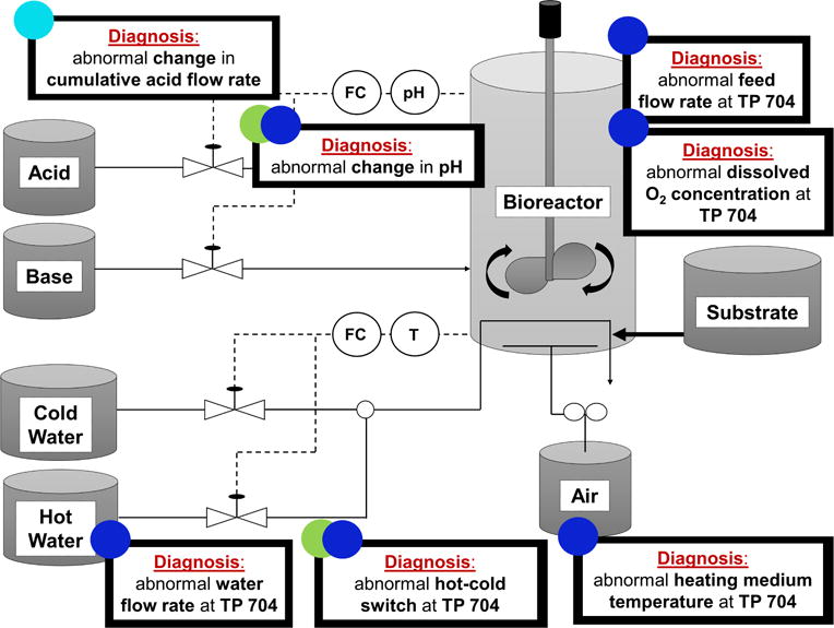
Diagnosis of Fault 8 (pH sensor drift) with One-step Rolling Time Horizon based Approach at selected Sample Bins. TP represents Time Point. The color codes indicate the sample bin index which is compatible with the Figure 8. (Cyan: Sample Bin 40, Green: Sample Bin 80, Blue: Sample Bin 120).

Figure 13.

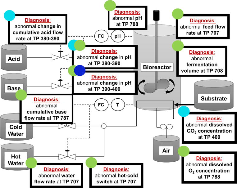
Diagnosis of Fault 8 (pH sensor drift) with Two-step Rolling Time Horizon based Approach at selected Sample Bins. TP represents Time Point. The color codes indicate the sample bin index which is compatible with the Figure 9. (Cyan: Sample Bin 40, Green: Sample Bin 80, Blue: Sample Bin 120).

Figure 14.

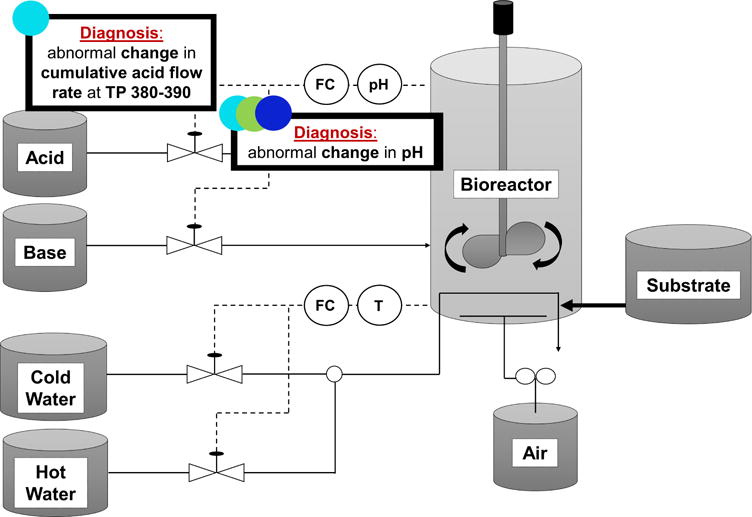
Diagnosis of Fault 8 (pH sensor drift) with Evolving Time Horizon based Approach at selected Sample Bins. TP represents Time Point. The color codes indicate the sample bin index which is compatible with the Figure 10. (Cyan: Sample Bin 40, Green: Sample Bin 80, Blue: Sample Bin 120).

Highlights.

• A novel data-driven framework using nonlinear Support Vector Machine-based feature selection is proposed for fault detection and diagnosis in batch processes.

• The proposed framework is applied on a comprehensive benchmark dataset comprising of 22,600 batches with 15 faults, and normal operation.

• Fault and time-specific models are trained for simultaneous fault detection and diagnosis with three distinct time horizon approaches: one-step rolling, two-step rolling and evolving.

A Appendix

Figure A1.

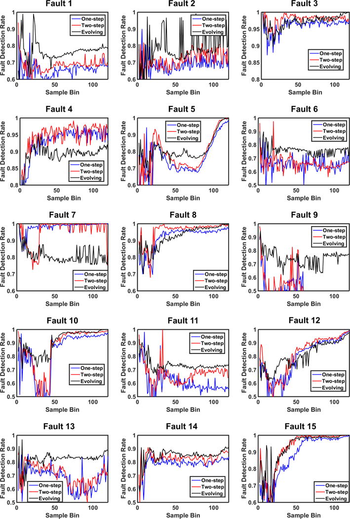
Comparison of the Fault Detection Rates for All Faults along the Batch Process with respect to One-step Rolling, Two-step Rolling, and Evolving Time Horizon approaches

References

- 1.Floudas CA, Niziolek AM, Onel O, Matthews LR. Multi-Scale Systems Engineering for Energy and the Environment: Challenges and Opportunities. AIChE Journal. 2016;62(3):602–623. [Google Scholar]
- 2.Yin S, Ding SX, Xie X, Luo H. A review on basic data-driven approaches for industrial process monitoring. IEEE Transactions on Industrial Electronics. 2014;61(11):6414–6428. [Google Scholar]
- 3.He QP, Wang J. Statistical process monitoring as a big data analytics tool for smart manufacturing. Journal of Process Control. 2017 [Google Scholar]
- 4.Helu M, Libes D, Lubell J, Lyons K, Morris K. Enabling smart manufacturing technologies for decision-making support. Proc ASME Des Eng Tech Conf. 2016;1B doi: 10.1115/DETC2016-59721. [DOI] [PMC free article] [PubMed] [Google Scholar]
- 5.Chiang L, Lu B, Castillo I. Big Data Analytics in Chemical Engineering. Annual Review of Chemical and Biomolecular Engineering. 2017;8(1):63–85. doi: 10.1146/annurev-chembioeng-060816-101555. [DOI] [PubMed] [Google Scholar]
- 6.Reis M, Gins G. Industrial Process Monitoring in the Big Data/Industry 4.0 Era: from Detection, to Diagnosis, to Prognosis. Processes. 2017;5(3):35. [Google Scholar]
- 7.Beck DAC, Carothers JM, Subramanian VR, Pfaendtner J. Data Science: Accelerating Innovation and Discovery in Chemical Engineering. AIChE Journal. 2016;62(5):1402–1416. [Google Scholar]
- 8.Chiang LH, L RE, D BR. Advanced Textbooks in Control and Signal Processing. Springer; 2001. Fault Detection and Diagnosis in Industrial Systems. [Google Scholar]
- 9.Venkatasubramanian V, Rengaswamy R, Yin K, Kavuri SN. A review of process fault detection and diagnosis. Computers & Chemical Engineering. 2003;27(3):293–311. [Google Scholar]
- 10.Isermann R. Model-based fault-detection and diagnosis status and applications. Annual Reviews in Control. 2005;29(1):71–85. [Google Scholar]
- 11.Takeda K, Shibata B, Tsuge Y, Matsuyama H. The improvement of fault diagnosis algorithm using signed directed graph. IFAC Proceedings. 1994;27(5):351–356. IFAC Symposium on Fault Detection, Supervision and Safety for Technical Processes SAFEPROCESS’94, Espoo, Finland, 13–16 June. [Google Scholar]
- 12.Liu Y-K, Wu G-H, Xie C-L, Duan Z-Y, Peng M-J, Li M-K. A fault diagnosis method based on signed directed graph and matrix for nuclear power plants. Nuclear Engineering and Design. 2016;297(Supplement C):166–174. [Google Scholar]
- 13.Chen M, Zheng AX, Lloyd J, Jordan MI, Brewer E. Failure diagnosis using decision trees; International Conference on Autonomic Computing, 2004 Proceedings; May 2004.pp. 36–43. [Google Scholar]
- 14.Venkatasubramanian V, Vaidyanathan R, Yamamoto Y. Process fault detection and diagnosis using neural networksi. steady-state processes. Computers & Chemical Engineering. 1990;14(7):699–712. [Google Scholar]
- 15.Silvestri G, Verona FB, Innocenti M, Napolitano M. Fault detection using neural networks. Neural Networks, 1994 IEEE World Congress on Computational Intelligence, 1994 IEEE International Conference on. 1994 Jun;6:3796–3799. vol.6. [Google Scholar]
- 16.Zhao Q, Xu Z. Design of a novel knowledge-based fault detection and isolation scheme. IEEE Transactions on Systems, Man, and Cybernetics, Part B (Cybernetics) 2004 Apr;34:1089–1095. doi: 10.1109/tsmcb.2003.820595. [DOI] [PubMed] [Google Scholar]
- 17.Ge Z, Song Z, Gao F. Review of Recent Research on Data-Based Process Monitoring. Industrial & Engineering Chemistry Research. 2013;52(10):3543–3562. [Google Scholar]
- 18.Venkatasubramanian V, Rengaswamy R, Kavuri SN. A review of process fault detection and diagnosis part II: Qualitative models and search strategies. Computers & Chemical Engineering. 2003;27(3):313–326. [Google Scholar]
- 19.Qin SJ. Survey on data-driven industrial process monitoring and diagnosis. Annual Reviews in Control. 2012;36(2):220–234. [Google Scholar]
- 20.Nomikos P, MacGregor JF. Monitoring batch processes using multiway principal component analysis. AIChE Journal. 1994;40(8):1361–1375. [Google Scholar]
- 21.Dong Y, Qin SJ. A novel dynamic pca algorithm for dynamic data modeling and process monitoring. Journal of Process Control. 2017 [Google Scholar]
- 22.Rato TJ, Rendall R, Gomes V, Chin ST, Chiang LH, Saraiva PM, Reis MS. A Systematic Methodology for Comparing Batch Process Monitoring Methods: Part I-Assessing Detection Strength. Industrial and Engineering Chemistry Research. 2016;55(18):5342–5358. [Google Scholar]
- 23.Bakshi BR. Multiscale pca with application to multivariate statistical process monitoring. AIChE journal. 1998;44(7):1596–1610. [Google Scholar]
- 24.Li F, Church G, Janakiram M, Gholston H, Runger G. Fault detection for batch monitoring and discrete wavelet transforms. Quality and Reliability Engineering International. 2011;27(8):999–1008. [Google Scholar]
- 25.Yu H, Khan F, Garaniya V. A sparse pca for nonlinear fault diagnosis and robust feature discovery of industrial processes. AIChE Journal. 2016 [Google Scholar]
- 26.PlOVOSO MJ, KOSANOVICH KA. Applications of multivariate statistical methods to process monitoring and controller design. International Journal of Control. 1994;59(3):743–765. [Google Scholar]
- 27.Nomikos P, MacGregor JF. Multi-way partial least squares in monitoring batch processes. Chemometrics and Intelligent Laboratory Systems. 1995;30(1):97–108. InCINC ’94 Selected papers from the First International Chemometrics Internet Conference. [Google Scholar]
- 28.Kruger U, Dimitriadis G. Diagnosis of process faults in chemical systems using a local partial least squares approach. AIChE Journal. 2008;54(10):2581–2596. [Google Scholar]
- 29.Li G, Qin SJ, Zhou D. Geometric properties of partial least squares for process monitoring. Automatica. 2010;46(1):204–210. [Google Scholar]
- 30.Kano M, Tanaka S, Hasebe S, Hashimoto I, Ohno H. Monitoring independent components for fault detection. AIChE Journal. 2003;49(4):969–976. [Google Scholar]
- 31.Chiang LH, Russell EL, Braatz RD. Fault diagnosis in chemical processes using fisher discriminant analysis, discriminant partial least squares, and principal component analysis. Chemometrics and Intelligent Laboratory Systems. 2000;50(2):243–252. [Google Scholar]
- 32.Detroja KP, Gudi RD, Patwardhan SC, Roy K. Fault detection and isolation using correspondence analysis. Industrial & Engineering Chemistry Research. 2006;45(1):223–235. [Google Scholar]
- 33.Detroja KP, Gudi RD, Patwardhan SC. Data reduction and fault diagnosis using principle of distributional equivalence. 2011 International Symposium on Advanced Control of Industrial Processes (ADCONIP) 2011 May;:30–35. [Google Scholar]
- 34.Ghosh K, Ramteke M, Srinivasan R. Optimal variable selection for effective statistical process monitoring. Computers & Chemical Engineering. 2014;60:260–276. [Google Scholar]
- 35.Van Impe J, Gins G. An extensive reference dataset for fault detection and identification in batch processes. Chemometrics and Intelligent Laboratory Systems. 2015;148:20–31. [Google Scholar]
- 36.Wang R, Edgar TF, Baldea M, Nixon M, Wojsznis W, Dunia R. A geometric method for batch data visualization, process monitoring and fault detection. Journal of Process Control. 2017 [Google Scholar]
- 37.Cortes C, Vapnik V. Support-vector networks. Machine Learning. 1995;20(3):273–297. [Google Scholar]
- 38.Birol G, Ündey C, Çinar A. A modular simulation package for fed-batch fermentation: Penicillin production. Computers & Chemical Engineering. 2002;26(11):1553–1565. [Google Scholar]
- 39.Vapnik VN. The Nature of Statistical Learning Theory. New York, NY, USA: Springer-Verlag New York; 1995. [Google Scholar]
- 40.Scholkopf B, Smola AJ. Learning with Kernels: Support Vector Machines, Regularization, Optimization, and Beyond. Cambridge, MA, USA: MIT Press; 2001. [Google Scholar]
- 41.Guzman Y. PhD thesis. Princeton University; Princeton, NJ: 2016. Theoretical Advances in Robust Optimization, Feature Selection, and Biomarker Discovery. [Google Scholar]
- 42.Sobieszczanski-Sobieski J, Barthelemyy J-F, Riley KM. Sensitivity of optimum solutions of problem parameters. AIAA journal. 1982;20(9):1291–1299. [Google Scholar]
- 43.Barthelemy J-F, Sobieszczanski-Sobieski J. Optimum sensitivity derivatives of objective functions in nonlinear programming. AIAA Journal. 1983;21(6):913–915. [Google Scholar]
- 44.Castillo E, Mínguez R, Castillo C. Sensitivity analysis in optimization and reliability problems. Reliability Engineering & System Safety. 2008;93(12):1788–1800. [Google Scholar]
- 45.Guyon I, Weston J, Barnhill S, Vapnik V. Gene selection for cancer classification using support vector machines. Machine learning. 2002;46(1):389–422. [Google Scholar]
- 46.Chang C-C, Lin C-J. Libsvm: a library for support vector machines. ACM transactions on intelligent systems and technology (TIST) 2011;2(3):27. [Google Scholar]
- 47.Kieslich CA, Tamamis P, Guzman YA, Onel M, Floudas CA. Highly accurate structure-based prediction of hiv-1 coreceptor usage suggests intermolecular interactions driving tropism. PloS one. 2016;11(2):e0148974. doi: 10.1371/journal.pone.0148974. [DOI] [PMC free article] [PubMed] [Google Scholar]
- 48.Nomikos P, MacGregor JF. Monitoring batch processes using multiway principal component analysis. AIChE Journal. 1994;40(8):1361–1375. [Google Scholar]
Associated Data
This section collects any data citations, data availability statements, or supplementary materials included in this article.