deepNF: deep network fusion for protein function prediction

Abstract

Motivation

The prevalence of high-throughput experimental methods has resulted in an abundance of large-scale molecular and functional interaction networks. The connectivity of these networks provides a rich source of information for inferring functional annotations for genes and proteins. An important challenge has been to develop methods for combining these heterogeneous networks to extract useful protein feature representations for function prediction. Most of the existing approaches for network integration use shallow models that encounter difficulty in capturing complex and highly non-linear network structures. Thus, we propose deepNF, a network fusion method based on Multimodal Deep Autoencoders to extract high-level features of proteins from multiple heterogeneous interaction networks.

Results

We apply this method to combine STRING networks to construct a common low-dimensional representation containing high-level protein features. We use separate layers for different network types in the early stages of the multimodal autoencoder, later connecting all the layers into a single bottleneck layer from which we extract features to predict protein function. We compare the cross-validation and temporal holdout predictive performance of our method with state-of-the-art methods, including the recently proposed method Mashup. Our results show that our method outperforms previous methods for both human and yeast STRING networks. We also show substantial improvement in the performance of our method in predicting gene ontology terms of varying type and specificity.

Availability and implementation

deepNF is freely available at: https://github.com/VGligorijevic/deepNF.

Supplementary information

Supplementary data are available at Bioinformatics online.

1 Introduction

Methods for automated protein function prediction allow us to maximize the utility of functional annotations derived from costly and time-consuming protein function characterization and large-scale genomics experiments. The accuracy of these methods has been improved with the advent of high-throughput experimental methods that have enabled construction of different types of genome-scale molecular and functional interaction networks, including protein–protein interaction networks, genetic interaction networks, gene co-expression networks and metabolic networks. Extracting biological information from the wiring patterns (topology) of these networks is essential in understanding the functioning of the cell and its building blocks-proteins. A key insight behind this approach is that function is often shared between proteins that physically interact (Sharan et al., 2007), have similar topological roles in the interaction networks (Milenković and Pržulj, 2008), or are part of the same complex or pathway (Chen et al., 2014).

Systematic benchmarking efforts, such as the critical assessment of functional annotation (CAFA) (Radivojac et al., 2013) and MouseFunc (Peña-Castillo et al., 2008), have shown that the current methods for protein function prediction use diverse approaches to train classifiers on a multitude of network-, sequence- and structure-based data sources to make predictions (Cozzetto et al., 2013). Due to the complementary nature of these different data sources, such techniques have been shown to be more accurate than those that use a single data source (Cozzetto et al., 2013; Lanckriet et al., 2004; Wass et al., 2012). However, the heterogeneous nature of biological networks, as well as their different levels of sparsity and noise, makes development of such techniques challenging. Here we focus on integrating only network-based features in order to limit the scope of the work better isolate general results aimed at biological networks, and to better compare to important recent works on biological network integration.

Most previous approaches for network integration either use probabilistic methods, like Bayesian inference (Franceschini et al., 2013; Lee et al., 2011), kernel-based methods (Yu et al., 2015) to fuse different protein–protein network types, derived from different proteomic and genomic data sources, into a single network. The resulting network, along with the set of proteins’ function labels, are fed into a kernel- or network-based classifier to derive functional associations of annotated proteins and generate hypotheses about unannotated proteins. For example, GeneMANIA (Mostafavi et al., 2008; Mostafavi and Morris, 2012) is a widely used semi-supervised network-based method that first integrates kernels of different network types into a single kernel by solving a constrained linear regression problem; then, it applies Gaussian label propagation on the resulting kernel to make label predictions. However, as pointed out by Cho et al. (2016), these methods suffer from the information loss incurred when combining all the network types into a single network. To overcome this problem, some approaches train individual classifiers on these networks and then use ensemble learning methods to combine their predictions (Yan et al., 2010). However, such methods do not typically take into account correlations between different data sources, and, unlike GeneMANIA, often suffer from learning time and memory constraints. Previous work has also benefited from considering the hierarchical structure of gene ontology (GO) (Barutcuoglu et al., 2006), using statistical principles to choose negative examples (i.e. proteins without a given function) (Youngs et al., 2013) or modeling the incomplete set of protein function annotations as a matrix completion or recommendation system problem (Gligorijević et al., 2014).

2 Related work

A recent study proposed Mashup (Cho et al., 2016), a network integration framework, to address the challenge of fusing noisy and incomplete interaction networks. Mashup takes as input a collection of protein–protein association networks and applies a matrix factorization-based technique to construct compact low-dimensional vector representation of proteins that best explains their wiring patterns across all networks. These vectors are then fed into a support vector machine (SVM) classifier to predict functional labels of proteins. The key step in Mashup is the feature learning step that constructs informative features that have been shown to be useful in multiple scenarios including highly accurate protein function and protein–protein interaction prediction.

There are several challenges to learning a useful low-dimensional network representation (also known as network embedding) while preserving the network structure. In particular, most protein–protein association networks are characterized by diverse connectivity patterns. Specifically, proteins with the same or similar functional annotations in these networks often exhibit a complex mixture of relationships, based both on homophily (close proximity to each other in the network) and structural similarity (similar local wiring patterns, regardless of the position in the network).

Thus, it is a challenging task to learn a low-dimensional embedding of proteins that preserves non-linear network structure while remaining predictive of protein functions. Even more challenging is the construction of such a compact low-dimensional embedding of proteins that is consistent across different protein functional and molecular interaction modalities (i.e. across different types of protein–protein association networks).

The majority of previous network embedding methods use shallow and linear techniques that encounter difficulty in capturing complex and highly non-linear network structure. These include methods such as node2vec (Grover and Leskovec, 2016) and DeepWalk (Perozzi et al., 2014) that are mainly used on social networks. Although it is theoretically possible for shallow neural networks to learn complex data structures (Ba and Caruana, 2014), it is often in practice not feasible. On the other hand, deep learning is a promising technique to deal with such problems, and has been shown to work well for problems such as speech recognition, natural language processing and image classification, as well as for several biological problems (Angermueller et al., 2016). Motivated by the recent success of deep learning techniques in learning powerful representations from complex data, a few recent studies propose using deep neural networks (DNNs) for computing network embeddings (Cao et al., 2016; Grover and Leskovec, 2016; Wang et al., 2016). DNNs apply multiple layers of non-linear functions to map input data into a low-dimensional space, thereby capturing highly non-linear network structure in efficient low-dimensional features. A multi-layer architecture of DNN is a key to learning richer network representation. The advantage of using DNNs has been demonstrated in learning embeddings of large-scale social networks for performing different tasks, such as link prediction, network clustering and multi-label classification (Cao et al., 2016; Wang et al., 2016). However, none of these methods can construct embeddings by handling different network modalities (i.e. types, views), i.e. these methods cannot be used for integrative analysis. Thus, we propose deep Network Fusion, deepNF (also pronounced deep enough), an integrative framework for learning compact low-dimensional feature representation of proteins that (i) captures complex topological patterns across multiple protein–protein association networks, and that (ii) is used to derive functional labels of proteins. To explicitly address the diversity of protein–protein interaction network types, we use separate layers for handling each network type in the early parts of the deep autoencoder, later connecting all the layers into a single bottleneck layer from which we extract features to predict protein function for different species. Similar to Mashup, in the last phase, deepNF trains an SVM on the resulting features to predict each protein function label.

deepNF is based on a multimodal deep autoencoder (MDA) to integrate different heterogeneous networks of protein interactions into a compact, low-dimensional feature representation common to all networks. An autoencoder is a special type of neural network that is composed of two parts: (i) an encoding part, in which the input data is transformed into low-dimensional features, and (ii) a decoding part, in which those features are mapped back to the input data (Vincent et al., 2010). Our method, deepNF, has the following conceptual advances: (i) it preserves the non-linear network structure by applying multiple layers of non-linear functions, composing the DNN architecture of deepNF, thereby learning a richer network representation; (ii) it handles noisy links present in the networks, as autoencoders have also been shown to be effective denoising systems capable of constructing useful representations from corrupted data (Vincent et al., 2010); and (iii) it is efficient and scalable as it uses the MDA to learn low-dimensional protein features from all networks in a fully unsupervised way and independently of the function prediction task. This allows for the use of the entire dataset in the training of the MDA, resulting in high-quality features. Our method enables semi-supervised approaches to function prediction. Here we demonstrate such a semi-supervised approach to function prediction task by training an SVM for each function on these features. Additionally, the reduced dimension of the extracted features makes the training of the SVMs computationally efficient.

We apply this method on human and yeast STRING networks to construct a compact low-dimensional representation containing high-level protein features. For each species, we perform 5-fold cross validation, as well as temporal holdout validation, in which we train our method on GO annotations from 2015 and test it on those from 2017. We report the performance of our method for different DNN architectures. We contrast the performance of our method with the state-of-the-art network integration methods, Mashup and GeneMANIA. We report a significant improvement of deepNF over these methods on both yeast and human protein function annotations. We also report a significant improvement in performance when training deepNF on all STRING networks together than when training it on each individual STRING network, demonstrating the success of our integrative strategy.

To the best of our knowledge, this is the first method that uses a deep multimodal technique to integrate diverse biological networks. We demonstrate that deep learning methods offer the great advantage of being able to capture non-linear information contained in large-scale biological networks, and that using such techniques could lead to improved network representations. Features learned by using these methods not only lead to substantial improvements in protein function prediction accuracy but also our temporal holdout results indicate that our method can also be used for prioritizing novel experimental target proteins for a given function.

3 Approach

In this section, we introduce our framework for predicting protein functions from multiple networks, deepNF, including the preprocessing step, adopted from Cao et al. (2016), and the cornerstone of our method, the MDA. In the pre-processing step the structural information of each network is converted into a high-dimensional vector representation that is used as input to the MDA. We also provide implementation details and a description of our testing schemes: cross-validation and temporal holdout validation.

4 Materials and methods

We consider a set of N = 6 undirected weighted STRING networks whose connectivity patterns are represented by a set of symmetric adjacency matrices $\{{\mathbf{A}}^{(1)},{\mathbf{A}}^{(2)},\dots ,{\mathbf{A}}^{(N)}\}$. Each matrix, ${\mathbf{A}}^{(j)}\in {ℝ}^{n\times n}$, is constructed over the same set of proteins. deepNF learns low-dimensional latent feature representation of n proteins, ${\mathbf{H}}_c\in {ℝ}^{d_c\times n}$ (where $d_c\ll n$), shared across all networks. In order to do so, the method follows three steps (see Fig. 1): (i) it converts structure of each network into a high-quality vector representation by first applying the Random Walk with Restarts (RWR) method and then constructing a Positive Pointwise Mutual Information (PPMI) matrix capturing structural information of the network; (ii) it fuses PPMI matrices of networks by using the MDA, and from the middle layer extracts a low-dimensional feature representation of proteins; (iii) it predicts protein function by training an SVM classifier on the low-dimensional features computed in the previous step. An outline of the procedure is provided in Supplementary Algorithm S1. We provide details of each step below.

Fig. 1.

Method overview. In the first step networks are converted into vectors after the RWR method (left). After this preprocessing step, the networks are combined via our MDA (right). Low-dimensional features are then extracted from the middle layer of the MDA and used to train a final classifier (bottom)

4.1 Random walk-based network representation

To capture network structural information and to convert it to high-dimensional protein vector representation suitable for input to the MDA, we adopt the approach of Cao et al. (2016) and further modify it for multiple networks. For each network $j\in \{1,\dots N\}$ we construct high-quality vector representations of proteins, ${\mathbf{X}}^{(j)}\in {ℝ}^{n\times n}$, preserving potentially complex, non-linear relations among the network nodes. To do so, we first use the RWR model to capture network structural information and to characterize the topological context of each protein. We chose the RWR method for converting network structure into initial node vector representations over the previously proposed sampling-based procedure in node2vec (Grover and Leskovec, 2016) and DeepWalk (Perozzi et al., 2014), because these methods are computationally more intense and require additional hyperparameter fitting. The RWR approach can be formulated as the following recurrence relation:

$${\mathbf{p}}_i^{(t)}=\alpha {\mathbf{p}}_i^{(t-1)}\widehat{\mathbf{A}}+(1-\alpha ){\mathbf{p}}_i^{(0)},$$ (1)

where ${\mathbf{p}}_i^{(t)}$ is a row vector of protein i, whose kth entry indicates the probability of reaching the kth protein after t steps, ${\mathbf{p}}_i^{(0)}$ is the initial one-hot vector, α is the probability of restart controlling the relative influence of local and global topological information of a network represented by adjacency matrix, A, and $\widehat{\mathbf{A}}$ is the one-step probability transition matrix obtained by applying row-wise normalization of the adjacency matrix.

To compute the node representation, ${\mathbf{r}}_i$, we adopt the strategy proposed by Cao et al. (2016), which is given by the following formula:

$${\mathbf{r}}_i=\sum _{t=1}^T{\mathbf{p}}_i^{(t)},$$ (2)

where T is the total number of RW steps. Repeating this process for every node $i\in \{1,\dots n\}$ in the network j, results in a representation matrix $\mathbf{R}\in {ℝ}^{n\times n}$, characterizing the probability of co-occurrence of network nodes. Such a representation captures high-order proximities of network nodes. To best see this, we can choose α = 1, and, by using Equation (2), show that the representation matrix has the following form:

$$\mathbf{R}=\widehat{\mathbf{A}}+{\widehat{\mathbf{A}}}^2+\cdots +{\widehat{\mathbf{A}}}^T,$$

where ${\widehat{\mathbf{A}}}^k=\underset{k}{\underbrace{\widehat{A}·\widehat{A}\dots ·\widehat{A}}}$ is the k-order proximity matrix.

Next, from the probabilistic co-occurrence matrix, ${\mathbf{R}}^{(j)}$, of network, j, we construct a vector representation of proteins by computing the PPMI matrix defined as:

$${\mathbf{X}}_{lm}^{(j)}=\max \left(0,{\hspace{0.17em}\text{log}\hspace{0.17em}}_2\left(\frac{{\mathbf{R}}_{lm}^{(j)}{\sum }_l{\sum }_m{\mathbf{R}}_{lm}^{(j)}}{{\sum }_l{\mathbf{R}}_{lm}^{(j)}{\sum }_m{\mathbf{R}}_{lm}^{(j)}}\right)\right).$$ (3)

It is important to note that this process occurs as a first step and thus the RWR representation is mitigating the sparsity of some individual network types prior to the deeper integration described in next steps below.

4.2 Integrating networks with MDA

Although the above approach is fast, it results in protein features that still represent individual networks in a high-dimensional space. As such, these features cannot be readily used for protein function prediction. Here, we propose to use MDA for integrating multiple networks represented by PPMI matrices, reducing their dimension and creating protein features, extracted from all networks that are more suitable for training a classifier and predicting protein functions.

The MDA constructs a low-dimensional feature representation of n proteins, that best approximates all networks, $j\in \{1,\dots ,N\}$, by projecting their PPMI matrices, ${\mathbf{X}}^{(j)}\in {ℝ}^{n\times n}$, using multiple non-linear activation functions, into a common feature space, ${\mathbf{H}}_c\in {ℝ}^{d_c\times n}$ (i.e. a common bottleneck layer in DNN architecture of the MDA, see Fig. 1). Following the standard definition of autoencoders (Vincent et al., 2010), we formulate the encoding and decoding part of the MDA as follows:

• Encoding: in the first hidden layer of the MDA, we first compute low-dimensional non-linear embedding, ${\mathbf{H}}^{(j)}\in {ℝ}^{d_j\times n}$, for each network $j\in \{1,\dots ,N\}$:

  $${\mathbf{H}}_{\text{encode}}^{(j)}=\sigma ({\mathbf{W}}_{\text{encode}}^{(j)}{\mathbf{X}}^{(j)}+{\mathbf{B}}_{\text{encode}}^{(j)}),$$

  where ${\mathbf{W}}_{\text{encode}}^{(j)}\in {ℝ}^{d_j\times n}$ and ${\mathbf{B}}_{\text{encode}}^{(j)}\in {ℝ}^{d_j\times n}$ are weight and bias matrices, respectively, and $\sigma (x)=\frac{1}{1+e^{-x}}$ is the sigmoid activation function. We compute a common feature representation by applying multiple non-linear functions (i.e. by stacking a series of hidden layers in the MDA) on the feature representation obtained by concatenating features from all networks obtained in the previous step (i.e. the previous layer):

  $${\mathbf{H}}_{c,1}=\sigma ({\mathbf{W}}_1[{\mathbf{H}}^{(1)},\dots ,{\mathbf{H}}^{(N)}]+{\mathbf{B}}_1),$$

  where $\left[{\mathbf{H}}^{(1)},\dots ,{\mathbf{H}}^{(N)}\right]$ are the concatenated activation matrices (one for each network) of the previous layers. There can be L layers after this step that would be described using the following equation:

  $${\mathbf{H}}_{c,l+1}=\sigma ({\mathbf{W}}_l{\mathbf{H}}_{c,l}+{\mathbf{B}}_l),$$

  where $l\in \{1,\dots ,L\}$ is the layer number for the successive integrated embeddings.
• Decoding: we first compute the larger common representation ${\mathbf{H}}_{c,L+1}$ from the last encoding common layer ${\mathbf{H}}_{c,L}$ described by the same equation above, with the same number of decoding layers as the number of encoding layers L. We then compute individual representations for each network ${\mathbf{H}}_{\text{decode}}^{(j)}$ described in the following equation:

  $${\mathbf{H}}_{\text{decode}}^{(j)}=\sigma ({\mathbf{W}}_{\text{decode},1}^{(j)}{\mathbf{H}}_{c,2L}+{\mathbf{B}}_{\text{decode},1}^{(j)}).$$

  We then compute reconstructed PPMI matrices, ${\widehat{\mathbf{X}}}^{(j)}$, for each network, $j\in \{1,\dots ,N\}$, by mapping the individual representations, ${\mathbf{H}}_{\text{decode}}^{(j)}\in {ℝ}^{d_c\times n}$ to the original space, by applying the following equation:

  $${\widehat{\mathbf{X}}}^{(j)}=\sigma ({\mathbf{W}}_{\text{decode},2}^{(j)}{\mathbf{H}}_{\text{decode}}^{(j)}+{\mathbf{B}}_{\text{decode},2}^{(j)}).$$

  Please also refer to Figure 1 for an example of a seven-layer MDA with corresponding notations.

The aim of the MDA method is to find optimal $\widehat{\theta }$ that minimizes the reconstruction loss, $L(\theta )$, between each original and reconstructed PPMI matrix:

$$\widehat{\theta }=\underset{\theta }{\text{argmin}}L(\theta )=\underset{\theta }{\text{argmin}}\sum _{j=1}^{N}l({\mathbf{X}}^{(j)},{\widehat{\mathbf{X}}}^{(j)}),$$ (4)

where $l(*)$ is the sample-wise binary cross-entropy function and $\theta =\{{\mathbf{W}}_{\text{encode}}^{(j)},{\mathbf{B}}_{\text{encode}}^{(j)},{\mathbf{W}}_{\text{decode}}^{(j)},{\mathbf{B}}_{\text{decode}}^{(j)},{\mathbf{W}}_l,{\mathbf{B}}_l\}$, for $j\in \{1,\dots ,N\}$ and $l\in \{1,\dots ,2L\}$ is the set of all parameters in both the encoding and decoding parts of our model to be learned in the training process.

A key step of our approach is the second step in the encoding part of the MDA that constructs a common feature representation by first denoising each individual network (by constructing their corresponding low-dimensional feature representations) and then projecting them into a common feature space.

The loss function (Equation 4) can be optimized by standard back-propagation algorithm. We use mini-batch stochastic gradient descent with momentum for training the MDA. We also explore the performance of the MDA with different batch sizes, learning rates and different architectures (i.e. number and sizes of hidden layers). Values of all hyperparameters are provided in Supplementary Section S3. After the training of the MDA is done, we extract the low-dimensional features, ${\mathbf{H}}_{c,L}\in {ℝ}^{d_c\times n}$, from its bottleneck layer.

4.3 Predicting protein function from multiple networks

We model the problem of protein function prediction as a multi-label classification problem. We use the compressed features, ${\mathbf{H}}_{c,L}$, computed in the previous step, to train an SVM classifier to predict probability scores for each protein. We use the SVM implementation provided in the LIBSVM package (Chang and Lin, 2011). To measure the performance of the SVM on the compressed features, we adopt two evaluation strategies: (a) 5-fold cross validation and (b) temporal holdout validation.

In the 5-fold cross validation, we split all annotated proteins into a training set, comprising 80% of annotated proteins, and a test set, comprising the remaining 20% of annotated proteins. We train the SVM on the training set and predict the function of the test proteins. We use the standard radial basis kernel (RBF) for the SVM and perform a nested 5-fold cross validation within the training set to select the optimal hyperparameters of the SVM (i.e. γ in the RBF kernel and the weight regularization parameter, C) via grid search. All performance results are averaged over 10 different CV trials.

In the temporal holdout validation, we use the protein GO annotations from 2015 and 2017 to form training, validation and test sets. We form the training set from proteins whose annotations did not change from 2015 to 2017. We form the test set from the proteins that did not have any annotations in 2015 but gained annotations in 2017. We use the same setup for the SVM classifier as in 5-fold cross validation. To fit the hyperparameters of the SVM, we created a validation set comprising proteins who had annotations in 2015 but also gained new annotations in 2017. We choose the optimal hyperparameters based on the SVM performance on the validation proteins, and report the final results on the test proteins. The performance results are averaged over 1000 bootstraps of the test set.

We compare the performance of our method with two state-of-the art methods, Mashup and GeneMANIA. For each method, we apply the validation strategies described earlier. We use the following metrics to evaluate the prediction performance: (i) Accuracy (ACC), that measures the percentage of test proteins that were correctly predicted (i.e. a protein is correctly predicted if the set of its predicted functions exactly match the set of its known functions); (ii) Micro-averaged F1 score (F1) is computed in the same way as in Cho et al. (2016); (iii) Micro-averaged area under the precision-recall curve (m-AUPR) is computed by first vectorizing the protein–function matrices of predicted scores and known binary annotations, and then computing the AUPR by using these two vectors; Macro-AUPR (M-AUPR) is computed by first computing the AUPR for each function separately, and then averaging these values across all functions. Here, we do not consider receiver operating characteristic curves as protein labels are highly skewed, and AUPR is less biased in that case and thus better choice (Davis and Goadrich, 2006).

4.4 Data pre-processing

To make the cross-validation performance comparison of deepNF with Mashup fair, we use the exact same dataset (i.e. the six STRING networks and functional annotations) used in the Mashup paper (Cho et al., 2016). The basic network measures and properties of the STRING networks are provided in Supplementary Table S1. Also, we report the results of the methods on both yeast and human STRING networks. The functional annotations for yeast are taken from Munich Information Center for Protein Sequences (MIPS) [again, this is done to make a perfect comparison to validations performed in Cho et al. (2016)] and they are organized into three functional categories: Level 1 (consisting of 17 most general functional categories), Level 2 (consisting of 74 functional categories) and Level 3 (consisting of 153 most specific functional categories). All functional annotations for human are taken from GO. Similar to yeast, they were arranged into three functional categories, i.e. categories containing GO terms annotating 11–30 (covering 153 molecular function (MF), 262 biological process (BP) and 82 cellular component (CC) GO terms), 31–100 (covering 72 MF, 100 BP and 48 CC GO terms) and 101–300 (covering 18 MF, 28 BP and 20 CC GO terms) proteins, respectively.

To compile function annotation data for temporal holdout validation, we use a similar strategy as proposed in the CAFA challenge (Jiang et al., 2016; Radivojac et al., 2013). We obtain protein annotation data for 2015 (release 145) and 2017 (release 167) year from UniProt-GOA (Huntley et al., 2015) database. For each ontology (i.e. MF, BP and CC) and each model organism (i.e. yeast and human), we create our training, validation and test sets of proteins as described above, specifically: the training set is formed of proteins whose annotations did not change from 2015 to 2017, the test set comprises proteins who did not have any annotations in 2015 and gain at least one new annotation in 2017, and the validation set comprises proteins that had annotations in 2015 but also gained new annotations in 2017. We consider only GO terms that gained at least 10 test and 10 validation proteins in 2017 and that have between 10 and 300 training proteins. The number of training, validation and test proteins, as well as the number of functions for MF, BP and CC, for yeast and human, are summarized in Supplementary Table S2.

5 Results

Here, we use cross-validation and temporal holdout to evaluate deepNF and compare its performance to GeneMANIA and Mashup. In all of our experiments, we set $\alpha =0.98$ in the RWR step of our method as this leads to the best performance results on the validation set across all function label types and architectures tested for both organisms. Other choices of α (e.g. $\alpha =1.0$) have been shown to result in lower quality of extracted features (see Section 4.1) (Cao et al., 2016). Regarding the number of RW steps (T), for many different real-world networks the choice of T = 3 has been shown to lead to the best performance as suggested by Cao et al. (2016) and Mostafavi et al. (2012). After conducting the same empirical study (for T = 2, 3, 4, 5), we have also selected T = 3, in all our experiments, as it leads to the best performance (data not shown).

In the training of the MDA, we explore different layer configurations (also known as architectures) and regularization parameters. Values of all the hyperparameters and the details of the MDA training strategy as well as of the SVM training are provided in Supplementary Section S3.

5.1 Cross-validation performance

To evaluate the quality of the low-dimensional features extracted from the bottleneck layer of the MDA (Fig. 1), we run the same 5-fold cross-validation procedure as in the Mashup paper (Cho et al., 2016). We train the MDA for different layer configurations for Yeast and Human STRING networks. The performance of our method in yeast and human for different architectures is provided in Supplementary Figures S2 and S4, respectively.

We find that the features obtained from the five-layer architecture (two encoding, one feature layer and two decoding layers) of the MDA, trained on the Yeast STRING networks, lead to the best performance in terms of the m-AUPR across all three levels of MIPS ontology. Performance of the same model on different annotation levels of the MIPS hierarchy, in comparison to GeneMANIA and Mashup, is summarized in Figure 2. We observe that deepNF significantly outperforms (rank-sum P-value < 0.01) (Note here that using the rank-sum test could sometimes lead to over-optimistic results as the GO terms are not fully independent.) both Mashup and GeneMANIA in terms of m-AUPR at different levels of MIPS hierarchy. Consistent improvement of deepNF is also achieved in terms of accuracy (i.e. the percentage of test proteins with all the predicted functions exactly matching the corresponding known functions). Namely, deepNF accurately assigns known functions to 31.3% of proteins, as opposed to 23.6% for GeneMANIA and 25.5% for Mashup in Level 1 of MIPS annotations. Note that this is a more rigorous measure than the accuracy measure used in the Mashup paper by Cho et al. (2016), which only considers top predicted functions for each protein. Although we observe clear improvements in terms of m-AUPR across all levels of MIPS annotations, however, in terms of M-AUPR in Levels 2 and 3 of MIPS annotations, deepNF performs comparably to Mashup.

Fig. 2.

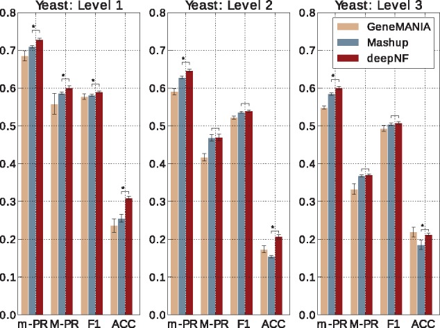
Cross-validation performance of our method in integrating yeast networks. Performance of our method, with the MDA architecture [6 × n, 6 × 2000, 600], in 5-fold cross validation in comparison to function prediction performance of the state-of-the-art integration method, Mashup, and GeneMANIA. The notation ‘6 × Z’, where Z is the number of features for each network, indicates that the embeddings for each network are separate, whereas single integers mean that the layers have already been concatenated. Performance is measured by the area under the precision-recall curve, summarized over all GO terms both under the micro-averaging (m-PR) and macro-averaging (M-PR) schemes; F1 score and accuracy (ACC). Performance of the methods is shown separately for MIPS yeast annotations for Level 1 (left), Level 2 (middle) and Level 3 (right). The error bars are computed based on 10 trials. Asterisks indicate where the performance of deepNF is significantly higher than the performance of Mashup (rank-sum P-value < 0.01)

The cross-validation performance of the seven-layer MDA (three enconding, one feature layer and three decoding) applied on Human STRING networks in comparison to Mashup and GeneMANIA is shown in Figure 3. Our method significantly outperforms the other two methods, in terms of all four measures, for the MF-GO terms belonging to the most specific (i.e. annotating between 11 and 30 proteins) categories. For the MF-GO terms belonging to the most general (i.e. annotating between 101 and 300 proteins) categories, we observe significantly higher performance in all measures except in accuracy. Specifically, in terms of accuracy, GeneMANIA significantly outperforms both deepNF and Mashup (rank-sum P-value = 0.004 < 0.01). The performance of our method for MF-GO terms with between 31 and 100 proteins annotated in the training set) is comparable to Mashup, except in terms of F1 measure for which our method achieves significantly better performance.

Fig. 3.

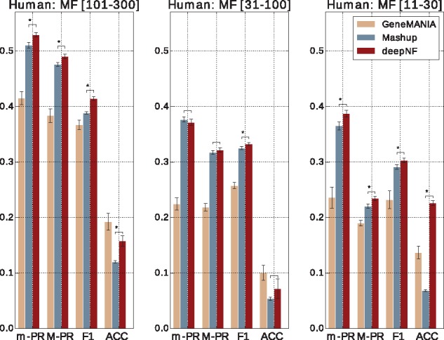
Cross-validation performance of our method in integrating human networks. Performance of our method, with the MDA architecture [6 × n, 6 × 2500, 9000, 1200], in 5-fold cross validation in comparison to function prediction performance of the state-of-the-art integration method, Mashup, and GeneMANIA. Performance is measured by the area under the precision-recall curve, summarized over all GO terms both under the micro-averaging (m-AUPR) and macro-averaging (M-AUPR) schemes; F1 score and accuracy (ACC). Performance of the methods is shown separately for all three ontologies of GO, i.e. MF, BP and CC, where each ontology is further divided into three levels annotating 101–300, 31–100 and 11–30 proteins, respectively

Similar results are also observed for both BP and CC ontologies (shown in Supplementary Fig. S6). The observed improvement in accuracy of our method in comparison to Mashup can be partially attributed to the high quality of protein features extracted from the complex topology of STRING networks in the hierarchical manner. Unlike Mashup, which utilizes a shallow matrix factorization-based technique to construct compact protein feature representation, deepNF utilizes a hierarchical way of feature construction by incorporating intermediate layers in the MDA architecture (see Fig. 1). The de-noising property of the multimodal autoencoder underlying our method leads to better detection of relevant features from individual networks and, ultimately, to a better final integrated feature representation. To further demonstrate the usefulness of such an approach in feature construction, we also apply our method on individual STRING networks (i.e. without integration). Namely, we train a deep autoencoder on each STRING network, separately, and further assess the quality of the extracted low-dimensional features of each individual network in predicting protein functions. The integrative performance and the performance on individual networks of our method in comparison to Mashup is shown in Figure 4 for both yeast and human STRING networks.

Fig. 4.

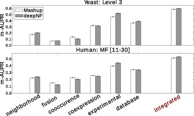
Integrating multiple networks outperforms individual networks in protein function prediction. We compare the cross-validation performance of our method applied on individual STRING networks, measured by m-AUPR, with the performance of Mashup. The upper panel shows the performance results on the most specific MIPS terms (Level 3) for each individual STRING network of yeast, whereas, the bottom panel shows the performance results on the most specific MF-GO terms for each individual STRING network of human. The low-dimensional features of these networks are extracted from the bottleneck layer of autoencoders trained on each individual network. We use architecture [n, 2000, 600] for yeast STRING networks, and architecture [n, 2500, 9000, 1200] for human STRING networks. In addition to individual network performance, we also show the integrative performance of both methods

5.2 Temporal holdout performance

Unlike the cross-validation procedure, which randomly divides protein set into folds used for training and testing the model, the temporal holdout procedure divides proteins into training and test sets based on their annotations at two different widely separated time points, where older annotations are used for training and newer ones are used for testing the model. The temporal holdout approach ensures a more ‘realistic’ scenario of function prediction. The study of individual MDA architectures shows that the five-layer architecture of the MDA in yeast and seven-layer architecture of the MDA in human yields the best performance in terms of M-AUPR across different GO ontologies (see Supplementary Figs S2 and S4). The temporal holdout validation performance of our method with these architectures is shown in Figures 5 and 6, for yeast and human data, respectively. The performance of both methods on MF terms is higher than for BP terms, which is in line with the findings reported by previous studies (Jiang et al., 2016; Radivojac et al., 2013).

Fig. 5.

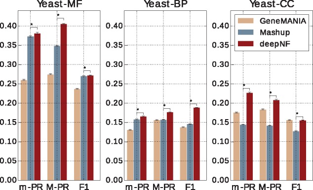
Temporal holdout validation performance of our method in integrating Yeast STRING networks. Performance of our method with the MDA architecture [6 × n, 6 × 2000, 600], in temporal holdout validation in comparison to function prediction performance of GeneMANIA and Mashup. Performance is measured by the area under the precision-recall curve (AUPR) both under micro-averaging (m-AUPR) and macro-averaging (M-AUPR) and F1 score. The results are averaged over 1000 boostraps of the test set; asterisks indicate where the performance of deepNF is significantly better than the performance of Mashup (rank-sum P-value < 0.01)

Fig. 6.

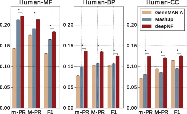
Temporal holdout validaton performance of our method in integrating Human STRING networks in comparison to GeneMANIA and Mashup. Performance of our method, with the MDA architecture [6 × n, 6 × 2500, 9000, 1200], in temporal holdout validation in comparison to function prediction performance of GeneMANIA and Mashup. Performance is measured by the area under the precision-recall curve (AUPR) both under micro-averaging (m-AUPR) and macro-averaging (M-AUPR) and F1 score. The results are averaged over 1000 boostraps of the test set; asterisks indicate where the performance of deepNF is significantly better than the performance of Mashup (rank-sum P-value < 0.01)

We observe that deepNF substantially outperforms both Mashup and GeneMANIA in temporal holdout validation. We observe clear improvements in both yeast and human data across all three types of ontologies. Interestingly, unlike in cross-validation, where Mashup significantly outperforms GeneMANIA, GeneMANIA achieves higher performance results than Mashup in temporal holdout validation, especially for the CC ontology for both yeast and human data. This could be due to the very high density of CC annotations; i.e. there are on average 2.42 CC-GO terms per protein in the training set (out of total 11 CC-GO terms), as opposed to 2.54 MF-GO terms (out of total 20 MF-GO terms) and 3.77 BP-GO terms per protein (out of total 43 BP-GO terms), in the temporal holdout set in yeast, which can be handled better by label propagation framework, such as GeneMANIA, than by Mashup. However, the high density of annotations per protein is more suitable for a deep learning technique, such as our method, which achieves higher performance, across all metrics, than both GeneMANIA and Mashup.

We further explored the performance of our method on specific individual GO terms used in the temporal holdout study. The AUPR values of the 20 MF-GO terms computed from the features of Yeast STRING networks are shown in Figure 7. From the figure, we can observe that deepNF achieves higher AUPR performance than Mashup for the majority of MF-GO terms. We observe similar results also for BP- and CC-GO terms (see Supplementary Fig. S8), and also for Human STRING networks in all three ontologies (see Supplementary Fig. S9). Specifically, we observe that the majority of MF-GO terms considered in our temporal holdout set that were descendants of the GO term ‘binding’ perform better with a deep architecture (i.e. deepNF) than with a shallow one (i.e. Mashup), whereas, the quite opposite situation is observed with MF-GO terms that were descendants of ‘transporter activity’. Surprisingly, this is in contrast with one of the findings reported in Radivojac et al. (2013), where the authors observe that most function prediction methods consistently perform worse on the ‘binding’ related terms than on the ‘transporter activity’ related terms. This indicates that our method provides complementary results in comparison to the methods presented in the paper. Furthermore, by looking into CC-GO terms (Supplementary Fig. S8), we observe that the majority of CC-GO terms associated with ‘membrane’ perform better with our method than with Mashup, whereas the situation is opposite for CC-GO terms associated with ‘vesicle’.

Fig. 7.

Temporal holdout validation shows significant difference in the performance of our method vs. Mashup in predicting individual yeast MF-GO terms. For each MF-GO term we show the Mashup’s and deepNF’s performance (five-layer MDA), measured by the AUPR. The lower panel shows the difference in the performance of these two methods. The names of the GO terms are shown on the x-axis

To further strengthen the performance of our method, we conduct an additional comparison study of our method with three baseline methods whose results are provided in Supplementary Section S7. In particular, to show the importance of the MDA step, as a first baseline method (termed SVM-PPMI), we train the SVM on the high-dimensional protein vectors (i.e. n-dimensional, where n is the number of nodes in the network) obtained from the PPMI matrices. We use the same grid search procedure for choosing the optimal parameters (γ of the RBF kernel, and the regularization parameter C) as in deepNF. As a second baseline method, we implement a linear-SVM trained on the random projections of the input PPMI vectors (termed SVM-RND_proj). We adopt Gaussian random projection method (Ailon and Chazelle, 2009) to reduce the dimensionality of the input vectors by projecting the original input space (PPMI matrices) on a randomly generated matrix with components drawn from the Gaussian distribution, $N\left(0,\frac{1}{n_{\text{dim}}}\right)$, where n_dim = 600 (for Yeast) and n_dim = 1200 (for Human). And finally, to show the importance of the PPMI step and the difference between our preprocessing step and the Mashup’s preprocessing step, we run our method on the RWR diffusion states (with restart probability 0.5) generated by Mashup’s preprocessing step (deepNF-mRWR). The performance of these baseline methods together with the performance of deepNF on the MF, BP and CC ontologies for both Human and Yeast STRING networks are shown in Supplementary Fig. S10. The performance of deepNF-mRWR is much lower than deepNF and all other baseline methods. This is not surprising given that the deepNF cost function (i.e. binary cross entropy) is more suitable for PPMI profiles than it is for RWR diffusion probabilities (for which the authors of the Mashup paper use KL-divergence). The results indicate that the performance of the SVM on the raw PPMI features is surprisingly good (even comparable in some cases with the performance of the SVM on the autoencoder features). Given that deepNF outperforms both SVM-RND_proj and SVM-PPMI baseline methods, we can say, with high certainty, that the embeddings learned by MDA, that capture the topological information of all N = 6 networks, are not trivially memorizing the input vectors and are not random projections.

6 Conclusion

Recent wide application of high-throughput experimental techniques has provided complex high-dimensional complementary protein association data; the wide availability of this data has in turn driven a need for protein function prediction methods that can take advantage of this heterogeneous data. We present here, for the first time, a deep learning-based network fusion method, deepNF, for constructing a compact low-dimensional protein feature representation from a multitude of different networks types. These features allow us to use out-of-the-box machine learning classifiers such as SVMs to accurately annotate proteins with functional labels.

deepNF extracts features that are highly predictive of protein function, which is attributed to the fact that the method relies on a deep learning technique that can more accurately capture relevant protein features from the complex, non-linear interaction networks. However, Mashup, an innovative previous method that combines protein networks to generate features for function prediction, cannot extract features that have this quality.

We present an extensive performance analysis comparing our method with competing protein function prediction methods. In addition to cross-validation, the analysis includes a temporal holdout validation evaluation similar to the measures in CAFA. Double-blind field-wide validation efforts (like CAFA) have demonstrated the utility of such temporal holdouts and established them as the most accepted way of performance comparison for protein function prediction methods. We show that deepNF outperforms previous methods (Mashup and GeneMANIA) in both human and yeast organisms, in multiple levels of specificity of GO and MIPS terms.

Given that the features generated by deepNF are task-independent, they can be used for other applications besides protein function prediction. Additionally, our method is not limited to only network integration: in future work, we hope to explore integrating other data types such as protein sequences and structures, represented as similarity networks, using our framework in order to make more accurate predictions of protein function.

References

- Ailon N., Chazelle B. (2009) The fast Johnson Lindenstrauss transform and approximate nearest neighbors. SIAM J. Comput., 39, 302–322. [Google Scholar]
- Angermueller C. et al. (2016) Deep learning for computational biology. Mol. Syst. Biol., 12, 878.. [DOI] [PMC free article] [PubMed] [Google Scholar]
- Ba J., Caruana R. (2014) Curran Associates, In: Conference Proceedings: Advances in Neural Information Processing Systems, Curran Associates, Inc., Montreal, Canada, pp. 2654–2662. [Google Scholar]
- Barutcuoglu Z. et al. (2006) Hierarchical multi-label prediction of gene function. Bioinformatics, 22, 830–836. [DOI] [PubMed] [Google Scholar]
- Cao S. et al. (2016) Deep neural networks for learning graph representations In: Proceedings of the Thirtieth AAAI Conference on Artificial Intelligence, AAAI’16, pp. 1145–1152. AAAI Press, Phoenix, AZ, USA. [Google Scholar]
- Chang C.-C., Lin C.-J. (2011) Libsvm: a library for support vector machines. ACM Trans. Intell. Syst. Technol., 2, 1–27. [Google Scholar]
- Chen B. et al. (2014) Identifying protein complexes and functional modules: from static ppi networks to dynamic ppi networks. Brief. Bioinformatics, 15, 177–194. [DOI] [PubMed] [Google Scholar]
- Cho H. et al. (2016) Compact integration of multi-network topology for functional analysis of genes. Cell Syst., 3, 540–548.e5. [DOI] [PMC free article] [PubMed] [Google Scholar]
- Cozzetto D. et al. (2013) Protein function prediction by massive integration of evolutionary analyses and multiple data sources. BMC Bioinformatics, 14, S1. [DOI] [PMC free article] [PubMed] [Google Scholar]
- Davis J., Goadrich M. (2006) The relationship between precision-recall and roc curves In: Proceedings of the 23rd International Conference on Machine Learning, ICML ’06, pp. 233–240, ACM, New York, NY, USA. [Google Scholar]
- Franceschini A. et al. (2013) String v9.1: protein-protein interaction networks, with increased coverage and integration. Nucleic Acids Res., 41, D808–D815. [DOI] [PMC free article] [PubMed] [Google Scholar]
- Gligorijević V. et al. (2014) Integration of molecular network data reconstructs gene ontology. Bioinformatics, 30, i594–i600. [DOI] [PMC free article] [PubMed] [Google Scholar]
- Grover A., Leskovec J. (2016) Node2vec: scalable feature learning for networks In: Proceedings of the 22Nd ACM SIGKDD International Conference on Knowledge Discovery and Data Mining, KDD ’16, pp. 855–864, ACM, New York, NY, USA. [DOI] [PMC free article] [PubMed] [Google Scholar]
- Huntley R.P. et al. (2015) The goa database: gene ontology annotation updates for 2015. Nucleic Acids Res., 43, D1057–D1063. [DOI] [PMC free article] [PubMed] [Google Scholar]
- Jiang Y. et al. (2016) An expanded evaluation of protein function prediction methods shows an improvement in accuracy. Genome Biol., 17, 184. [DOI] [PMC free article] [PubMed] [Google Scholar]
- Lanckriet G.R. et al. (2004) A statistical framework for genomic data fusion. Bioinformatics, 20, 2626–2635. [DOI] [PubMed] [Google Scholar]
- Lee I. et al. (2011) Prioritizing candidate disease genes by network-based boosting of genome-wide association data. Genome Res., 21, 1109–1121. [DOI] [PMC free article] [PubMed] [Google Scholar]
- Milenković T., Pržulj N. (2008) Uncovering biological network function via graphlet degree signatures. Cancer Informatics, 6, CIN.S680.. [PMC free article] [PubMed] [Google Scholar]
- Mostafavi S., Morris Q. (2012) Combining many interaction networks to predict gene function and analyze gene lists. Proteomics, 12, 1687–1696. [DOI] [PubMed] [Google Scholar]
- Mostafavi S. et al. (2008) GeneMANIA: a real-time multiple association network integration algorithm for predicting gene function. Genome Biol., 9, S4. [DOI] [PMC free article] [PubMed] [Google Scholar]
- Mostafavi S. et al. (2012) Labeling nodes using three degrees of propagation. Plos One, 7, e51947–e51910, 12. [DOI] [PMC free article] [PubMed] [Google Scholar]
- Peña-Castillo L. et al. (2008) A critical assessment of mus musculusgene function prediction using integrated genomic evidence. Genome Biol., 9, S2. [DOI] [PMC free article] [PubMed] [Google Scholar]
- Perozzi B. et al. (2014) Deepwalk: online learning of social representations In: Proceedings of the 20th ACM SIGKDD International Conference on Knowledge Discovery and Data Mining, KDD ’14, pp. 701–710. ACM, New York, NY, USA, 2014. [Google Scholar]
- Radivojac P. et al. (2013) A large-scale evaluation of computational protein function prediction. Nat. Methods, 10, 221–227. [DOI] [PMC free article] [PubMed] [Google Scholar]
- Sharan R. et al. (2007) Network-based prediction of protein function. Mol. Syst. Biol., 3, 1–13. [DOI] [PMC free article] [PubMed] [Google Scholar]
- Vincent P. et al. (2010) Stacked denoising autoencoders: learning useful representations in a deep network with a local denoising criterion. J. Mach. Learn. Res., 11, 3371–3408. [Google Scholar]
- Wang D. et al. (2016) Structural deep network embedding In: Proceedings of the 22Nd ACM SIGKDD International Conference on Knowledge Discovery and Data Mining, KDD ’16, pp. 1225–1234. ACM, New York, NY, USA. [Google Scholar]
- Wass M.N. et al. (2012) Combfunc: predicting protein function using heterogeneous data sources. Nucleic Acids Res., 40, W466–W470. [DOI] [PMC free article] [PubMed] [Google Scholar]
- Yan H. et al. (2010) A genome-wide gene function prediction resource for drosophila melanogaster. PLoS One, 5, 1–11. [DOI] [PMC free article] [PubMed] [Google Scholar]
- Youngs N. et al. (2013) Parametric bayesian priors and better choice of negative examples improve protein function prediction. Bioinformatics, 29, 1190–1198. [DOI] [PMC free article] [PubMed] [Google Scholar]
- Yu G. et al. (2015) Predicting protein function using multiple kernels. IEEE/ACM Trans. Comput. Biol. Bioinformatics, 12, 219–233. [DOI] [PubMed] [Google Scholar]
Associated Data
This section collects any data citations, data availability statements, or supplementary materials included in this article.